STUDYING AND
F
ORECASTING
T
RENDS FOR
C
RYPTOCURRENCIES
U
SING A
M
ACHINE
L
EARNING
APPROACH
J
OHAN
P
ETTER
M ¨
OLLER
Bachelor’s thesis
2018:K15
Faculty of Science
Centre for Mathematical Sciences
Numerical Analysis
CENTRUM
SCIENTIARUM
MA
THEMA
TICARUM
Lund University, Faculty of Science, Numerical Analysis
Bachelor thesis in Numerical Analysis
Studying and Forecasting Trends for
Cryptocurrencies Using a Machine Learning
Approach
Author :
Johan M¨
oller
Supervisor :
Alexandros Sopasakis
October 16, 2018
Abstract
We consider a technique involving Neural Networks in order to try to predict trends for cryptocurrencies such as Bitcoin, Ethereum etc. In that respect the project involves construction, design and training of a deep learning Neural Network based on historical trading data for these cryptocurrencies. Subse-quently we apply this trained network in order to better understand its ability to possibly forecast future trading trends.
Popul¨
arvetenskaplig sammanfattning
Genom att anv¨anda maskininl¨arning med fokus p˚a artificiella neuronn¨at ska vi f¨ors¨oka preidktera trender f¨or kryptovalutor, s˚a som Bitcoin, Ethereum etc. F¨or att genomf¨ora detta kr¨avs det att konstruera, designa och tr¨ana ett djupt neuronn¨at baserat p˚a tidigare data. Sedermera anv¨ands detta neuronn¨at f¨or att b¨attre f¨orst˚a maskininl¨arning och dess f¨orm˚aga att prediktera framtida trender.
Acknowledgment
I would like to thank my supervisor Alexandros Sopasakis for all the help, encourage and enthusiasm.
Contents
1 Introduction 6
1.1 Problem Statement . . . 7
2 Neural Network 8 2.1 Activation Function . . . 8
2.2 Training and Testing . . . 9
2.2.1 Example of Neural Network . . . 9
2.2.2 Backpropagation Algorithm . . . 9
3 Optimization of The Error Surface 12 3.1 Error Functions . . . 12
3.2 Optimization Algorithm . . . 12
3.2.1 Pseudocode for Adam Optimization Algorithm . . . 13
3.2.2 Algorithm Description . . . 13
3.3 Biases and Weights Exemplified . . . 16
3.3.1 Example of Backpropagation . . . 18
3.3.2 Pseudocode for Backpropagation . . . 20
4 Problems 20 4.0.1 Recall: Training and Testing Score . . . 20
4.1 Normalization . . . 21
4.2 Vanishing Gradient . . . 21
4.3 Overfit . . . 21
4.4 Dropout . . . 22
4.5 Regularization . . . 22
5 Universal Approximation Theorem 22 6 Comparison Model 23 6.1 Geometric Brownian Motion: . . . 23
6.2 Pseudocode for Brownian Simulation . . . 25
7 Rolling Prediction Forecast 26 7.1 Algorithm . . . 26
8 Result 27 8.1 Train and Test Score . . . 27
9 Predictions 31 9.1 Result from Rolling Prediction Forecast . . . 31
9.2 Comparison Method . . . 34
9.2.1 GBM Result . . . 34
9.2.2 Bitcoin GBM Plots . . . 35
9.2.3 Ethereum GBM Plots . . . 37
9.3 Neural Network Prediction versus True Change . . . 43
10 Comparison 47
11 Conclusion 48
11.1 Further work . . . 48
1
Introduction
Forecasting trends for assets such as cryptocurrencies is not an easy task. In this thesis the goal is to understand how a machine learning method can be used for forecasting trends of time series data. Machine learning is, in some sense, smart algorithms that can draw conclusions from data, i.e learn data patterns. Further, a Brownian motion will be used for forecasting trends of the same data. This method will be used as a comparison.
The author does not believe, what so ever, that one can easily predict the future of cryptocurrencies or similar assets by constructing a machine learning algorithm or Brownian paths for forecasting trends. The author does believe that machine learning is a powerful tool for comprehending data pattern. Cryptocurrencies are often in spotlight and then in context of wide volatility and high returns. Therefore, it seems interesting to see how a machine learning algorithm can be used for comprehend data pattern of such assets. The machine learning algorithm will involve neural networks and a rolling prediction forecast. Software such as: Keras, TensorFlow and Scikit-Learn are used for writing the algorithms. All code is written in Python.
In this thesis a regression method with supervised learning will be investigated. Regression meaning that the input map to an output and not a probability. Supervised learning meaning that the user must provide a label to each input so the algorithm can compare prediction output with true label. Subsequently, the algorithm will make predictions on data inputs which have no labels.
1.1
Problem Statement
In this thesis, a method for predicting the closing price using neural networks will be investigated. The prediction will be based on former closing prices. This method will be compared with another method, a Geometric Brownian Motion. LetX~ = X1, X2, X3, ..., Xtbe a vector of closing prices at certain time points fromi= 1, ..., t. Further, letF(·) denote a neural network. Can a neural net-work be used for forecasting trends of closing price of different cryptocurrencies,
~ˆ
X= Xˆt+1,Xˆt+2,Xˆt+3, ...,Xˆt+k
wherekis the prediction sequence length.
F( X1, X2, X3, ..., Xt
) = Xˆt+1,Xˆt+2,Xˆt+3, ...,Xˆt+k
2
Neural Network
Artificial neural networks (ANN) are designed to have layers. Layers consist of neuros, sometimes called nodes. In the first layer, the input layer, the neurons are sending the input further into the layers. The input is sometimes referred to as the input signal or just the signal. The signal is provided by the user. Each neuron in each layer is connected to each neuron in the next layer. Each connec-tion is a weight. A weight is an unknown variable. The weight is combined with the signal obtained from the previous layer. In each neuron two operations are executed. One summoning junction which sum the signals from previous layer combined with a weight. The second operation is called a “wrapper”. This is a function, called activation function. The activation function takes the signal as input The activation function is often a non-linear function which introduce non-linearity to the network. This is called for when the relation between input and output is non-linear. A smart choice of activation function may reduce the training time. Training is optimization of the difference between network out-put and desired outout-put with respect to the weights. Training is discussed and explained in subsection “Training and Testing” (2.2). The signal is traversed through the hidden layers. If the network has more than one hidden layer, the network is considered a deep learning neural network. When the signal has traversed through the hidden layers it reaches the final layer. The output layer. In the output layer each signals are summed. The output from the output layer is the network output. The network output is compared to the desired output. There is no optimal number of neurons or hidden layers. A rule of thumb is if the problem the network is designed to solve is non-linear or complex, (i.e the relations between input and output), a multilayered network may decrease the training time and increase the test result. A design suitable for the problem is found by trial and error.
2.1
Activation Function
The activation functions role is to introduce non-linearity to the network. This is called for when the relationship between input variable and output label is non-trivial. A couple of different activation functions are the following:
ReLU = max(0, x)
Sigmoid, σ(x) = 1 1 +e−x
tanh(x) = 2
1 +e−2x −1
Different activation functions fit different tasks better even though they all can be used for all tasks. For example,σ(x) fits classification problems better and ReLu fits better for a regression problem. It has been experimentally discovered the choice of activation function mostly affects training time (1).
2.2
Training and Testing
Training is done be evaluating the difference between network-output and tar-get and subsequently minimizing the differences. Tartar-get is the desired value. The training data and test data must be provided by the user. The user has data points which are divided into train and test data. these are often called training-set and test-set. The test-set is unseen to the network and used to val-idate the network ability to approximate the data. The training set is used for training through backpropagation. Throughout training the goal is to modify the weights, so the network-output approximate the target as good as possible. The targets are also given by the user. The target is sometimes called label or desired value.
2.2.1 Example of Neural Network
In figure below an artificial neural network with design 4-5-1 is considered. This is a figure which is supposed to simplify the understanding of how a network is functioning. The neurons which are exemplified by circles are the functions and the connections (the lines between the nodes) are the weights. In this network only one hidden layer is used, therefore it is considered a single layer feedforward neural network. Feedforward refers to the input is traversed from right to left (in this case). The output for the last neuron, the output layer, as compared to the target. The difference referred to as the error. The error is then propagated backwards to measure the error contribution in each neuron. This is what the algorithm aims to minimize.
Input #1 Input #2 Input #3 Input #4 Output Hidden layer Input layer Output layer 2.2.2 Backpropagation Algorithm
Backpropagation is the algorithm used for training networks, i.e minimize the difference between network output and target.
• xi denotes the input. Provided by the user.
• yˆi denotes neuron output.
• zi denotes network output.
• yi denotes target. Provided by the user.
• wi denotes weights. Set at random and the updated.
• wj0 denotes biases.
• E(·) denotes the error function, i.e the difference between network output and target value.
• δi denotes the error.
Define a neuron with input signal as:
aj= X
i
wjiˆyi+wj0 (2)
Remark that if ˆyi =xi ifaj =a1 asj = 1 implies the algorithm is in the first
layer.
Now, the activation function,f(·), is applied: ˆ
yj=f(aj) (3)
If ˆyj is located in the last layer, the output layer, ˆyj =zj. The error function1 is defined, the error function measures the difference between network output and target. E= n X j E(j) (4)
E is as function dependent on the signalsaj, hence:
E=E(a1, a2, ..., ak) (5) Look at equation (2) we see that the only unknown variable iswij. Hence,E=
E(a(w)). Now, differentiating the error function with respect to a particular weight,wij:
∂Ej
∂wij
(6) Using the chain rule2 the derivative is divided into two parts. Recall thatE
j is a function depending onaj which in its turn depends onwij, therefore:
∂E(j) ∂wij =∂E (j) ∂aj ∂aj ∂wij (7)
1Error function can be defined in different ways, see Section ”Error function” 2Recall chain rule:y=f(x), x=f(t), ∂y
∂t = ∂y ∂x
∂x ∂t
Define:
δj=
∂E(j) ∂aj
(8)
δj being the errors in neuronj.
Using Equation (2), one sees:
∂aj ∂wij = ˆyi (9) Hence: ∂E(j) ∂wij = ∂E (j) ∂aj ˆ yi (10) Recallδj =∂E (j) ∂aj , ∂E(j) ∂wij =δjyˆi (11)
In Equation (11) one can see that the derivatives are the product of the neuron output and the error from the previous layer (this is possible because we prop-agate backwards and neuron output is obtained from forward propagation done before). This can be calculated using the local derivative of the activation func-tion in,f0(·) becausef0(aj) = ˆyiwhere ˆyiis a neuron output from previous layer. Consider the signal traversed through the hidden layers ending up in the output layer. Here, the output is calledzk instead of ˆyi. kindicates that the signals is located in the output layer. The signal is now referred to asak. The error func-tion in current point is still referred to asE(j). The equation below (Equation.
(12)) is formed.
δk =
∂E(j)
∂zk
f0(ak) (12)
Equation (12) is the form to evaluate the deltas in the output layer. The deltas in the hidden layers are calculated using the formula:
δj =f0(aj) X
k
wkjδk (13)
This comes from splitting the derivatives of the error function using the chain rule once more, like:
∂E(j) ∂aj =δj ∂E(j) ∂aj =X k ∂E(j) ∂ak ∂ak ∂aj (14)
3
Optimization of The Error Surface
The graph of the error function (Eq. (4)) is referred to as the error surface. Training a network consist of more than finding the error contributions in each neuron. Training a network consists of optimizing the error surface. Through optimization the training algorithm aims to find weights which represent a min-ima on the error surface and therefore the weight update have more impact on training. Backpropagation delivers the gradients of the network.
3.1
Error Functions
Measuring the error is executed by different error functions. Two of the are Mean Squared Error (MSE) is one (Eq. (15)) and Absolute Error is another (Eq. (16)). E= 1 n n X i zi−yi 2 (15) E= 1 n n X i=1 |zi−yi| (16)
3.2
Optimization Algorithm
Different optimization algorithms are used. They are mostly different methods which originate from Newton’s method. One optimization algorithm commonly used to optimize the error surface of a neural network is Adam. The name Adam is derived fromadaptive moment estimation. Below an algorithm will be presented for using the Adam algorithm for calculating a minima of the error surface.
3.2.1 Pseudocode for Adam Optimization Algorithm
Algorithm 1Algorithm optimizingf(·) using Adam algorithm for optimizing
Result: wwhich minimizesf(·)
Require η: stepsize
β1, β2∈[0,1) : Exponential decay rates for the moment estimates
f(w): Function to be optimized
w0: Initial parameter vector
m0: Initial first moment vector
v0: Initial second moment vector
t= 0: First timestep
whilew not converged do
t=t+ 1 (1) gt=∇f(wt−1) (2) mt=β1mt−1+ (1−β1)gt (3) vt=β2vt−1+ (1−β2)gt2 (4) ˆ mt=1m−βtt 1 (5) ˆ vt=1−vtβt 2 (6) wt=wt−1−η(√mˆvˆt t+) (7) end 3.2.2 Algorithm Description
Below, a description of every step on Adam will be presented. 1. Timestep is updated
2. gtis the gradient of f(·) at timestept.
3. mtis the moment estimation. That is because the algorithm is minimizing the function with respect to its expected value. I.e, mt is the expected value of the gradient.
4. vtis the second moment, the mean squared calculated with:∇f (∂w∂f1)2,(∂w∂f2)2, ...
5. The estimation of the moment is biased and the term 1/1−β1t is
compen-sating for the bias-term.
mt= (1−β1) t X i=1 β1t−igi E[mt] =E " (1−β1) t X i=1 β1t−igi #
E[mt] =E(gt) " (1−β1) t X i=1 β1t−i #
Considert= 2. Then the above case ca be expandes as,
(1−β1) β12−1+β 2−2 1
= (1−β1)(β1+ 1) = 1−β12
This is true for allt, therefore the algorithm compensating with 1/1−βt
1 and becomes, E(mt) 1−βt 1 =E(gt) (17)
6. This is analogues to the case above.
7. Here,wtis updated and a new iteration is starting.
Empirically it has been shown that good hyperparameter settings are: β1= 0.9,
β2= 0.999 andη= 0.0001. For further improvements, η may be updated each
iteration as follows: ηt=η p 1−βt 2 1−βt 1 (18)
It has been shown that Adam is used preferably before other optimization al-gorithms in machine learning problems, due its efficiency in a high dimensional parameter space (9). Machine learning algorithms are often considered to often be in high dimensional parameter space since the connections between nodes quickly add up to many parameters.
Consider the Mean Squared Error,
M SE= 1/nX i (zi−yi)2= 1/n X i E(zi, yi).
TheM SEwould normally be a convex function. OurM SE however is depend-ing on function values dependdepend-ing on more variables, such as weights. Therefore
E(F(X, w~ ), y) where F(·) is a neural network,w is a vector of all weights and
~
X is the input vector. In generalF(·)is not convex and thereforeE(z, y) is not convex. This may cause a problem because the optimization algorithm does not guarantee a global minima. Research have shown that the importance to find a global minima decreases when the network structure becomes larger (6). If the structure is large the algorithm only needs to find a ”big-enough-minima”. With these explanations new questions arises. What is a ”big-enough-minima”? Which structure is considered large? A ”big-enough-minima” simply refers to a minima which as impact on training, i.e. lower the training and testing score. However, a structure is large or small is connected to the problem (6). These loosely defined problems and solutions may cause problems for the user to con-struct a network that is able to train well. To plot the errors each epoch is a
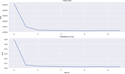
good indication if the network behaves as the user want. In Figure 1 a plot of a successfully trained network is shown. A common problem is overfitting. This can be detected if the train score is decreasing and test score is increasing. Remember, a low score is desirable.
Figure 1: Top plot: plot of training error. Bottom plot: plot of test score. Error converging to a small error after five epochs. No overfitting. Successfully trained network. If train loss would converge to zero but validation loss would increase, it would indicate overfitting.
In the plot Train Loss and Validation Loss refers to train score and respectively test score. A low score is desirable.
3.3
Biases and Weights Exemplified
In this section, the use of weights and biases will be exemplified. Note that bi-ases in this section do not refer to a bias estimation but a trainable parameter. A bias is added to make the neuron output more flexible.
Consider the input signal presented in Subsection 2.2.2.
aj=wjiˆyi+wj0 (19)
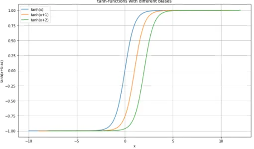
The weight makes the approximation more or less steep and the bias has the ability to move the signal on the x-axis, similar to a degree one polynomial. First, initial bias and weights are set at random.
Figure 2: tanh-functions with different biases added. Weights are set to be one. Here one sees how the bias may shift the activation function output on the x-axis. Blue curve: tanh(x), Orange curve: tanh(x+ 1), green curve: tanh(x+ 2).
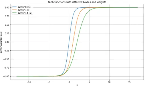
Figure 3: tanh-functions with different weights and biases, exemplifies the role of the weights. Here one sees how the weights make the activation function steeper and the biases shifting the curve on the x-axis. Blue curve: tanh(0.75x), Orange curve: tanh(x+ 1), green curve: tanh(1.5x+ 2).
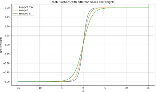
Figure 4: tanh-functions with different weights, exemplifies the role of the weights. Here one sees how the weights increases or decreases the steepness of the curve. Blue curve: tanh(0.75x), Orange curve: tanh(x), green curve: tanh(1.5x).
3.3.1 Example of Backpropagation
Consider a single layer network with one input neuron, two neurons in one hid-den layer and one output neuron in the output layer (see network below).
Input #1 Output Hidden layer Input layer Output layer
• f(·) denotes the activation function.
• xi denotes the input. Provided by the user.
• yˆi denotes neuron output.
• zi denotes network output.
• wi denotes weights. Set at random and the updated.
1. Forward propagate input x1 to the two neurons in the next layer, the
connections are weights. Here, only one operation is executed in each neuron. This is because there is only one input so no summation is needed for. For simplification the activation function used in the example is the identity.
f(x1, w1) =x1w1= ˆy1
f(x1, w2) =x1w2= ˆy2
(20)
2. Each neuron output, ˆy1 and ˆy2 is now send forward to the output layer
via two new connections, i.ew3 andw4.
f(y1, w3) = ˆy1w3= ˆy4
f(y2, w4) = ˆy2w4= ˆy5
(21)
3. Now the network output is calculated. Here the summering operation is demonstrated. Also, notice that in this step no weights are combined with the output from this neuron. That is because the output is not traversed forward. The connections between neurons are weights.
f(ˆy3,yˆ4) = ˆy3+ ˆy4=z1 (22)
4. In this step the outputz1 is compared with the target. Notice, y1 is the
target provided by the user.
z1−y1=δ5 (23)
5. δ5 is now propagated backwards and measure the error contribution in
each neuron. w4δ5=δ4 w3δ5=δ3 w2δ4=δ2 w1δ3=δ1 (24)
6. In this step each weight,wi, is updated. This is done by an optimization algorithm. Hereηdenotes the stepsize and ∂∂fyˆ
i is the partial derivative of
the activation function in each step.
w01=w1+η ∂f ∂yˆ1 x1δ1 w02=w2+η ∂f ∂yˆ2 x1δ2 w03=w3+η ∂f ∂yˆ3 ˆ y1δ3 w04=w4+η ∂f ∂yˆ4 ˆ y2δ4 (25)
7. w0iis the updated weight. This procedure is called an epoch. An epoch is an iteration of the algortihm.
3.3.2 Pseudocode for Backpropagation
Algorithm 2Algorithm for findingδ’s using backpropagation
Result: δj forj = 1,2...k layers
whilej≤k do
foreachwi,i= 1,2,...n. nnumber of connections do
if j = k then δj =f0(aj)∂z∂Ej else δj =f0(ai)Pjwijδj end end end end
4
Problems
Training a network consists of training many parameters and adjusting hyper-parameters. A hyperparameter is a parameter which can not be trained and must be set by the user. Setting hyperparameter is done by trial and error. Example of hyperparameters are the number of layers and neurons. Others are stepsize, iterations and batch size. Problems that occur are vanishing gradient, overfitting and optimization problems. The optimization problem is discussed in ”Optimization of The Error Surface”.
4.0.1 Recall: Training and Testing Score
Training score and test core is the score obtained from training and testing (sometimes referred to as training and validation ). Measured, in our case, with the Root Mean Squared Error-function. The train score is the score which measures how good the approximation is of the train-set (training data). This score is the mean difference between network output and target. The differ-ence between network output and target is what the training algorithm aims to minimize, i.e. obtaining low train score. If the network successfully trained the test score will be low. To get an understanding of what is a low score one may have to try different designs to try to find the lowest possible. Another good indicator of a low score is to plot the approximation and the target to get a visual if the approximation meets the user requirements. One example of a function measuring the error is the Root Mean Squared, see Equation (26).
Here,Xiis the network approximation of the target, yi. Error= v u u t 1 n n X i Xi−yi 2 (26)
4.1
Normalization
The train and test score will be lower if the data is normalized. Popular nor-malization ranges are: [0,1] and [−1,1]. If the data is not normalized the error surface will range over a wide interval. The optimization will be easier and better with normalized data and therefore lowering the train and test score.
4.2
Vanishing Gradient
Vanishing gradient occurs when the gradient which is propagated backwards through the network is too small and therefore has no impact on training. The reversed problem, exploding gradient, is when the gradient is too big and have too much impact. Due to the fact that the gradient is traversed backwards through the network, it is crucial for the training to beat vanishing/exploding gradient. If it occurs it affects the whole network.
To solve this problem one can utilize an activation function whose derivative is bounded and therefore the gradient will not blow up or explode. This can affect the network ability to solve a problem due to the fact that such activation function may obstruct the training. Instead of using such activation function one may try to design the network differently. More clever neurons have been developed to solve this problem. The most popular is a “Longs Short Term Memory”-network (LSTM-network). These networks are, while back propagat-ing, using adding operations and where multiplication is needed the network is using the identity. Which derivative is 1 by construction. These networks are hard to understand due to every neuron in an LSTM-network is in its turn a small network itself. We encourage the reader to seek information elsewhere because these networks are very powerful and do not need as much data as a feedforward network.
One detects vanishing gradient when training does not lower the test score.
4.3
Overfit
Overfit occurs when the network memorizes the data pattern and not compre-hend the data pattern. Overfit is detected by training score decreases while the test score increases. The best solution to this is to feed more data to the network. More data is in some cases not available and therefore other methods have to be selected. One may have to change the network design. A simpler
network may beat overfitting. This must be balanced well so the reversed prob-lem does not occur. This is the probprob-lem underfitting.
4.4
Dropout
Dropout simply refers to drop random neurons in an epoch. This implies that each neuron do not get updated every epoch and therefore the risk of overfitting decreases.
4.5
Regularization
Another way to combat overfitting is to add penalties to too strong signals. Consider again theM SE cost function with added a penalty:
M SE= 1 n n X i=1 ((zi−yi)2) +λ n X i=1 w2i
where λ is our penalty, w is our corresponding weight and z is the network output. Adding a penalty to too big signals and therefore their feature is not taken in too large consideration. This method is called regularization.
5
Universal Approximation Theorem
One classic theorem when it comes to the theory of neural networks is the
”Universal Approximation Theorem”. Universal Approximation Theorem was proven by George Cybenko in 1989 (10). George Cybenko stated that the
Universal Approximation Theorem only is true for Sigmoid activation function. In 1991 Kurt Hornik showed thatUniversal Approximation Theorem is true for an arbitrary activation function (10). Universal Approximation Theorem states that a neural network is a universal approximator, i.e. it can approximate an arbitrary function (10). The theorem is presented in this thesis for motivating the use of a neural network as an approximator in our case.
Theorem 5.1 (Universal Approximation Theorem (10)) Let g(·) be an arbi-trary activation function. let X ⊆ Rm and X compact. The space of
con-tinuous functions on X is denoted C(X). Then ∀f ∈ C(X), ∀ > 0 : ∃n ∈
N, wij, bi, φi∈R, i∈ {1, .., n}, j∈ {1, .., m}, such that: F(n)(x1, x2, ..., xm) = n X i=1 φig( m X j=1 wijxj+bi) (27)
as an approximation of the functionf(·);
||f −F(n)||<
With a compact space we mean a space closed and bounded. Here subscript
non the network,F(·). ndenotes the number of neurons the network consists of. Again, consider the input signal:
aj= X
i
wjiyˆi+wj0
If we wrap this signal in the activation function,g(·) we get:
g(X i
wjiˆyi+wj0)
and then sum all of these with a scalar we obtain: X j φjg( X i wjiyˆi+wj0)
This is the same approximator used inUniversal Approximation Theorem. Here,
iandj have changed places because of earlier notation, (see Equation (2)).
6
Comparison Model
For comparison a method involving a Monte Carlo simulation of a Brownian Motion is used below. A Geometric Brownian motion is used for modeling un-certainty and one of the fundamental equation for asset prices (2). The use of this method was inspired of the article ”Modeling the price of Bitcoin with geometric fractional Brownian motion: a Monte Carlo approach” by Mariusz Tarnopolski.
6.1
Geometric Brownian Motion:
A Geometric Brownian Motion is described as follows:
dXt=µXtdt+σXtdWt
X0=x0
(28)
The solution to this equation is known,
X(t) =x0exp ( µ−1 2σ 2 t+σW(t) ) (29)
X(t) denotes the stock price at time point t,µandσare constants, µis called drift parameter and σ is called volatility parameter. µ is the expected value and approximated as the arithmetic mean of the data (ˆµ) andσis the standard deviation calculated as:
σ=s= v u u t n X i=1 (xi−µˆ)2 n−1
xi is the observed value obtained from data. Wt is a sample from the normal distribution with varianceσ2 and expected value zero.
µandσ2are calculated from the variation in data, i.e the return between data
points. Calculated as follows:
Return= log xi
xi−1
Wherexi is the observed data.
Equation (29) is used for pricing Bitcoin using a Monte Carlo-approach. Mean-ing, the Brownian motion is simulated N times, where N denotes a constant that the user choose, i.e the number of paths. The expected value of the pre-dicted stock is calculated as the median of the values estimated at desired time step. The expected value is evaluated as the median comes from the fact that the return levels are log-normal distributed (2).
6.2
Pseudocode for Brownian Simulation
Algorithm 3Algorithm for producingnpaths of a Brownian motion.
Result: n paths for stock pricing
X0=initial value
number of simulation = N #set to an integer n. simulation = 0
Last T = a # last time step for prediction.
whilesimulation ≤number of simulations do
predicted prices = T = 0 t = 1 #time step whileT≤last T do XT =X0exp " µ−σ2 2 t+σ√t #
XT append to predicted prices T= T + 1
end end
7
Rolling Prediction Forecast
Neural networks are, today, used for stock prediction based on its well ability for non-linear mapping between input and output (5). This property makes a neural network suitable for time series analysis.
Rolling prediction forecast comes from using the predictions recursively, as fol-lows: F(X1, X2, ...Xt) =Xt+1 (30) F(X1, X2, ...Xt) = ˆXt+1 F(X2, ...Xt,Xˆt+1) = ˆXt+2 F(X3, ...Xt,Xˆt+1,Xˆt+2) = ˆXt+3...
7.1
Algorithm
Below a proposed algorithm for making a rolling prediction forecast will be pre-sented. Here,F(·) is the network which performs the prediction. The network is written in Keras and TensorFlow. Keras and TensorFlow are a machine learning software available for the programming language Python.
Algorithm 4Algorithm for a rolling prediction forecast
Result: Prediction forktime points
Require: Data,X~ Prediction length,k t= 1 whilet ≤k do ˆ Xt+1=F(X~) ~ X = appendXˆt+1toX~ ~
X =Drop first entry inX~ j=j+ 1
end
8
Result
Training, testing and prediction result will be presented for the different meth-ods and afterwards compared to the true outcome. Training score is the score the network achieves on training data, i.e. the data where the network is per-forming the training. This means that in the rolling prediction forecast the algorithm iterates over target data and not predicted data. Test score refers to the score achieved on testing, sometimes called validation. This measures how well the network performs on unseen data. This data still has a target value, meaning we can measure how well the network performs. During testing the network still iterates over true data. First when making forecasts about the future the algorithms iterates over predicted data points.
The score is measured using the function Root Mean Squared Error, ”RMSE”.
RM SE= v u u t 1 n n X i ( ˆXi−yi)2 (31)
Where ˆXi denotes network output. yi denotes the target.
8.1
Train and Test Score
Below the different score will be presented. Further, plots will be presented to indicate if the regression performs well or not.
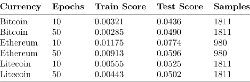
Table 1: Score, the square root of theM SE.
Currency Epochs Train Score Test Score Samples
Bitcoin 10 0.00321 0.0436 1811 Bitcoin 50 0.00285 0.0490 1811 Ethereum 10 0.01175 0.0774 980 Ethereum 50 0.00913 0.0596 980 Litecoin 10 0.00555 0.0525 1811 Litecoin 50 0.00443 0.0502 1811
Looking at the result from table 1, we see the score obtained from training and testing using different numbers of epochs, 10 and 50. Worth noticing is that the score increases with less data (score obtained from Ethereum). This seems intuitively correct due to the network has less training experience.
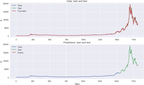
Figure 5: Network output on Bitcoin data (1811 samples). Top plot: network output compared with true data. Red curve is the true data. Blue curve is the network output on the train set (85 % of the data). network obtained train score, 0.00321 after ten epochs (measured using the root mean squared error). Indicating that the network trained well. Green curve: network output on test set. Test score: 0.0436. Another indication that the network performed well is that we almost do not see the network output, it is almost exactly looking as the red curve. Bottom plot: Only network output. Blue curve: network output on train set. Green curve: network output on test set. Orange curve: predictions for the five following days (see Section ”Predictions”).
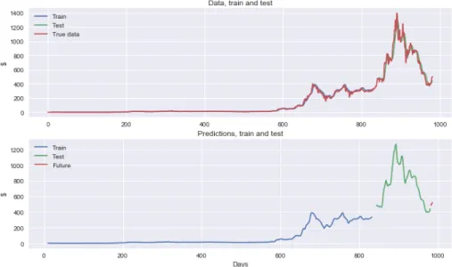
Figure 6: Network output on Ethereum data (980 samples). Top plot: network output compared with true data. Blue curve is the network output on the train set (85 % of the data). network obtained train score 0.00913 after ten epochs (measured using the root mean squared error). Green curve: network output on test set. Test score: 0.0596. An indication that the network performed well is that we almost do not see the network output, it is almost exactly looking as the red curve. Bottom plot: Only network output. Blue curve: network output on train set. Green curve: network output on test set. Orange curve: predictions for the five following days (see Section ”Predictions”).
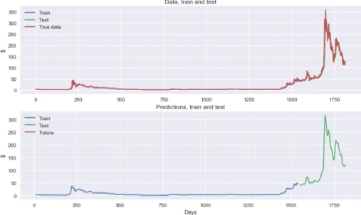
Figure 7: Network output on Litecoin data (1811 samples). Top plot: network output compared with true data. Blue curve is the network output on the train set (85 % of the data). Obtained train score, 0.00443 after ten epochs (measured using the root mean squared error). Green curve: network output on test set. Test score: 0.0502. An indication that the network performed well is that we almost do not see the network output, it is almost exactly looking as the red curve. Bottom plot: Only network output. Blue curve: network output on train set. Green curve: network output on test set. Orange curve: predictions for the five following days (see Section ”Predictions”).
9
Predictions
From Section ”Rolling Prediction Forecast” an algorithm for prediction was presented. In this section, the result will be presented. The predictions are for five days ahead. Here, as stated in section ”Rolling Predictions Forecast” the algorithm is iterating over predicted values.
9.1
Result from Rolling Prediction Forecast
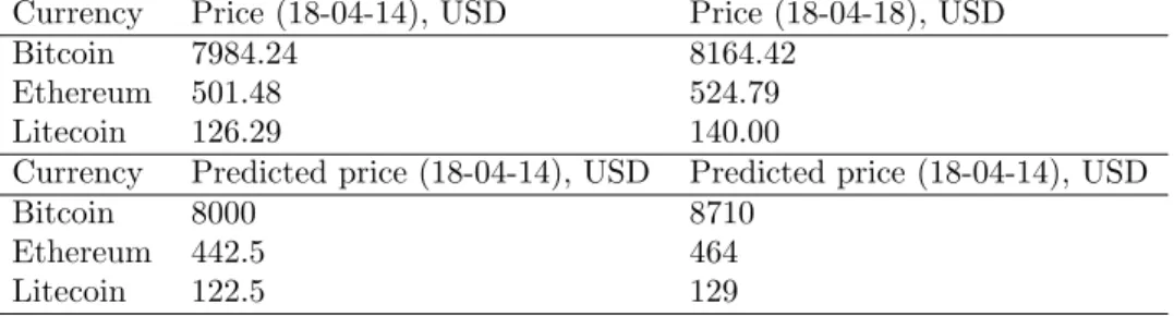
Table 2: True and predicted prices from 18-04-14 to 18-04-18. In this table we only take the neural network-method predictions in consideration.
Currency Price (18-04-14), USD Price (18-04-18), USD
Bitcoin 7984.24 8164.42
Ethereum 501.48 524.79
Litecoin 126.29 140.00
Currency Predicted price (18-04-14), USD Predicted price (18-04-14), USD
Bitcoin 8000 8710
Ethereum 442.5 464
Figure 8: Bitcoin: Predictions for the five following days, (April 14 to April 18, 2018). Network predict an increase of 10.89%. True change: 2.21%.
Figure 9: Ethereum: Predictions for the five following days, (April 14 to April 18, 2018). Network predict an increase of 4.90%. True change: 4.60%
Figure 10: Litecoin: Predictions for the five following days, (April 14 to April 18, 2018). Network predict an increase of 5.31%. True change: 10.85%.
9.2
Comparison Method
15000 simulated Geometric Brownian Motions are simulated and then the me-dian is calculated. The meme-dian is the expected price. Below a plots and result will be presented.
9.2.1 GBM Result
Table 3: Predicted price (pred.), predicted change (pred. change) and true change.
Currency Pred. (18-04-14) Pred. (18-04-18) Pred. change (%) True change (%)
Bitcoin 7986.00 8052.41 0.832 % 2.21 %
Ethereum 501.000000 508.823070 1.5614 % 4.60 % Litecoin 126.00 125.873274 -0.1005 % 10.85 %
9.2.2 Bitcoin GBM Plots
Below the paths, prediction and histogram of the Bitcoin will be presented.
Figure 12: Bitcoin: Histogram over last price. Red line is most likely price 18/4.
9.2.3 Ethereum GBM Plots
Below the paths, prediction and histogram of the Ethereum data will be pre-sented.
Figure 15: Ethereum: Histogram over last price. Red line is most likely price 18/4.
9.2.4 Litecoin GBM Plots
Below the paths, prediction and histogram of the Litecoin data will be presented.
Figure 18: Litecoin: Histogram over last price. Red line is most likely price 18/4.
9.3
Neural Network Prediction versus True Change
Below a table of predicted changes and true changes will presented.
Table 4: True and predicted prices from 18-04-14 to 18-04-18. Only the neural network-method predictions in consideration.
Currency Price (18-04-14), USD Price (18-04-18), USD
Bitcoin 7984.24 8164.42
Ethereum 501.48 524.79
Litecoin 126.29 140.00
Currency Predicted price (18-04-14), USD Predicted price (18-04-14), USD
Bitcoin 8000 8710
Ethereum 442.5 464
Litecoin 122.5 129
Table 5: True and predicted change. Only the neural network-method in con-sideration.
Currency True change (%) Predicted change (%)
Bitcoin 2.21% 10.89%
Ethereum 4.60% 4.90%
Figure 20: Bitcoin: True change for the five following days, (April 14 to April 18, 2018). True change: 2.21%. Predicted 10.89%. The network could not predict the drop after one day. Looking at the plots in Section ”Train and test score” the predicted values have a more smooth curve which indicates that the network seem to have problem detecting daily trends.
Figure 21: Ethereum: True change for the five following days, (April 14 to April 18, 2018) True change: 4.60%. Predicted change: 4.90%. The network has problem detecting daily trends.
Figure 22: Litecoin: True change for the five following days, (April 14 to April 18, 2018). True change: 10.85%. Predicted change 5.31%. The network has problem detecting daily trends.
10
Comparison
Here a table will be presented were the predicted change will be compared to each other, i.e the GBM prediction and neural network prediction, and the true change.
Table 6: Neural network (NN) and Geometric Brownian Motion (GBM) change and true change from April 14 to April 18.
Currency NN change (%) GBM change (%) True change (%)
Bitcoin 10.89% 0.832 % 2.21 %
Ethereum 4.90% 1.5614 % 4.60 %
Litecoin 5.31% -0.1005 % 10.85 %
In Table 6 the predicted changes from both methods and also the true changes from April 14 to April 18, 2018 are presented. In all cases the GBM made a too low prediction but predicted an increase with success in two cases. In one case the GBM predicted a negative change, although the currency did increase with 10.85%. The neural network prediction predicted an increase in all cases, even though the predictions are too small or too big.
11
Conclusion
From this result, we can tell that a machine learning algorithm involving neural networks may be used to comprehend the data of a time series such as the clos-ing price of a cryptocurrency. If the algorithm can be used for forecastclos-ing the price for five days ahead is too early to say. The algorithm must be evaluated over time to investigate the ratio of true prediction versus false prediction. If the algorithm can predict an increase or decrease with an accuracy larger than 50% we believe it is a successful algorithm. The author does not believe that just because the algorithm predicted an increase in all cases and it came true in all cases it is not an indication that the algorithm may be used successfully for trading cryptocurrencies. It may just be, and probably is, a lucky shot.
11.1
Further work
The algorithm can be improved. Now, the algorithm only takes the closing price as an input variable but, more variables should be used for evaluating the closing price. For example, market volume and open price. During the work with the algorithm, a classification algorithm was developed to predict a prob-ability which indicated an increase or decrease. Perhaps that would be more interesting than an algorithm constructed to predict the exact price. In this thesis a regression method was used based on the possibility to visualize the approximation.
Also, it is important to notice that the price of an asset such as cryptocur-rencies depends on much more variables than earlier data points. Some of these variables seem to be impossible to use for modeling the closing price. Such as political instability etc.
Such a algorithm will be developed and actual trading will be investigated with more common assets such as stocks.
12
References
References
[1] Jeff Heaton. Artificial Intelligence for Humans, Volume 3: Deep Learning and Neural Networks.Heaton Research Inc, St. Louis, 2015.
[2] Tomas Bj¨ork. Arbitrage Theory in Continuous Time Oxford University Press, 1998
[3] Mariusz Bernacki and Przemys law W lodarczyk. Principles of training multi-layer neural network using backpropagation.
http://home.agh.edu.pl/~vlsi/AI/backp_t_en/backprop.html, September 2004.
[4] Xiao Ding, Yue Zhang, Ting Liu and Junwen Duan. Deep Learning for Event-Driven Stock Prediction. Research Center for Social Computing and Information Retrieval, Harbin Institute of Technology, China, and Singapore University of Technology and Design, Singapore. 2015. p. 2327- 2333. [5] Takashi Kimoto, Kazuo Asakawa, Morio Yoda and Masakazu TakeokStock
Market Prediction System with Modular Neural Networks. INVESTMENT
TECHNOLOGY RESEARCH DIVISION. Tokyo, Japan.
[6] Grzegorz Swirszcz, Wojciech Marian Czarnecki and Razvan Pascan Local Minima in Training a Neural Network, London, UK
[7] Aur´elien G´eron.Hands-On Machine Learning with Scikit-Learn TensorFlow
O’REILLY, 2017
[8] Christopher M. Bishop. Pattern Recognition and Machine Learning.
Springer, 2009. p. 225-284
[9] Diederik P. Kingma and Jimmy Lei B.
ADAM: A METHOD FOR STOCHASTIC OPTIMIZATION.University of
Amsterdam, OpenAI and University of Toronto. 2015
[10] Bal´azs Csan´ad Cs´aji. Approximation with Artificial Neural Networks. E¨otv¨os Lor´and University, Hungary
[11] Mariusz Tarnopolski, Modeling the price of Bitcoin with geometric frac-tional Brownian motion: a Monte Carlo approach.Faculty of Physics, As-tronomy and Applied Computer Science, Jagiellonian University, Krakow, Poland Available at: https://arxiv.org/pdf/1707.03746.pdf
[12] Brown, Brewer, Kevin D.; Feng, Yi; and Kwan, Clarence C. Y. (2012) Geometric Brownian Motion, Option Pricing, and Simulation: Some Spreadsheet-Based Exercises in Financial Modeling, Spreadsheets in
Education (eJSiE): Vol. 5: Iss. 3, Article 4. Available at: http://