Theses
12-8-2019
Object Detection in High Resolution Aerial Images and
Object Detection in High Resolution Aerial Images and
Hyperspectral Remote Sensing Images
Hyperspectral Remote Sensing Images
Yilong LiangFollow this and additional works at: https://scholarworks.rit.edu/theses
Recommended Citation Recommended Citation
Liang, Yilong, "Object Detection in High Resolution Aerial Images and Hyperspectral Remote Sensing Images" (2019). Thesis. Rochester Institute of Technology. Accessed from
This Dissertation is brought to you for free and open access by RIT Scholar Works. It has been accepted for inclusion in Theses by an authorized administrator of RIT Scholar Works. For more information, please contact
Hyperspectral Remote Sensing Images
by
Yilong Liang
A dissertation submitted in partial fulfillment of the requirements for the degree of Doctor of Philosophy in the Chester F. Carlson Center for Imaging Science
College of Science
Rochester Institute of Technology December 8, 2019
Signature of the Author
Accepted by
ROCHESTER, NEW YORK CERTIFICATE OF APPROVAL
Ph.D. DEGREE DISSERTATION
The Ph.D. Degree Dissertation of Yilong Liang has been examined and approved by the dissertation committee as satisfactory for the
dissertation required for the Ph.D. degree in Imaging Science
Dr. Eli Saber, Dissertation Advisor
Dr. Panos Markopoulos, Dissertation Co-advisor
Dr. Nathan Cahill
Dr. Sildomar Monteiro
Dr. David Messinger
Dr. Anthony Harkin, External Chair
To my wife and child, for their accompanies and understandings. To my father and mother, for their endless supports and encouragements.
To my brother and sister, for always being there with me.
the Chester F. Carlson Center for Imaging Science and the Department of Electrical and
Microelectronic Engineering at Rochester Institute of Technology has been so special to
me and I really enjoy every aspect of it.
First of all, I would like to express my sincere gratitude to my advisor, Dr. Eli Saber,
for his mentorship and support during the graduate study. I learned a lot from the regular
discussions and his wisdom, insight, diligence in doing research.
I would like to thank my co-advisor, Dr. Panos Markopoulos, for his patience and
hands-on guidance, which have been extremely valuable in exploring new areas of the
research topic and improving my research publications. I would also like to thank Dr.
Nathan Cahill and Dr. Sildomar Monteiro, for their endless supports throughout every
aspect of my research, without which I cannot make it possible. I really miss the weekly
meetings with the professors, discussing my research progress and solving the problems
that I encounter. Their coding skills, mathematical expertise, and research capabilities
have taught me how to become a detailed-oriented researcher and helped me with the
deliveries of high-quality research work. I would also like to thank Dr. David Messinger
and Dr. Anthony Harkin, for their willingness to serve as my committee members. I
really appreciate their guidance when I started working on my research, which was very
beneficial in understanding the field of graph theory and mathematical modeling.
Special thanks go to the Department of Defense and RIT for their financial support,
which allows me to attend many international conferences and workshops, giving me the
opportunities to learn from experts from all over the world. In addition, I really appreciate
all the help from the stuff members in the department, especially Mrs. Elizabeth
wood, Mrs. Sue Chan, Mrs. Joyce French, Mrs. Patricia Vicari, Mrs. Florence Layton,
Mr. Kenneth Snyder, and Mr. James Stefano for their academic assistance and support.
Last but not least, I would like to say thank you to all the colleagues that I work with
in the image, video, and computer vision laboratory, especially Dr. Mustafa Jaber, Dr.
Sreenath Vantaram, Dr. Abdul Haleem Syed, Dr. Sankaranarayanan Piramanayagam,
Mr. Yang Hu, Mr. Osborn De Lima, Mr. Yansong Liu, Mr. Yue Wang, and Mr. Jobin
Mathew, for their help and accompanies. Their personalities, intelligence, and shared
Yilong Liang Submitted to the
Chester F. Carlson Center for Imaging Science in partial fulfillment of the requirements
for the Doctor of Philosophy Degree at the Rochester Institute of Technology
Abstract
With rapid developments in satellite and sensor technologies, there has been a dramatic
increase in the availability of remotely sensed images. However, the exploration of these
images still involves a tremendous amount of human interventions, which are tedious,
time-consuming, and inefficient. To help imaging experts gain a complete understanding
of the images and locate the objects of interest in a more accurate and efficient way, there
is always an urgent need for developing automatic detection algorithms. In this work,
we delve into the object detection problems in remote sensing applications, exploring
the detection algorithms for both hyperspectral images (HSIs) and high resolution aerial
images.
In the first part, we focus on the subpixel target detection problem in HSIs with
low spatial resolutions, where the objects of interest are much smaller than the image
pixel spatial resolution. To this end, we explore the detection frameworks that integrate
image segmentation techniques in designing the matched filters (MFs). In particular, we
propose a novel image segmentation algorithm to identify the spatial-spectral coherent
image regions, from which the background statistics were estimated for deriving the MFs.
Extensive experimental studies were carried out to demonstrate the advantages of the
proposed subpixel target detection framework. Our studies show the superiority of the
approach when comparing to state-of-the-art methods.
The second part of the thesis explores the object based image analysis (OBIA)
frame-work for geospatial object detection in high resolution aerial images. Specifically, we
generate a tree representation of the aerial images from the output of hierarchical
im-age segmentation algorithms and reformulate the object detection problem into a tree
matching task. We then proposed two tree-matching algorithms for the object detection
framework. We demonstrate the efficiency and effectiveness of the proposed tree-matching
based object detection framework.
In the third part, we study object detection in high resolution aerial images from a
machine learning perspective. We investigate both traditional machine learning based
framework and end-to-end convolutional neural network (CNN) based approach for
vari-ous object detection tasks. In the traditional detection framework, we propose to apply
the Gaussian process classifier (GPC) to train an object detector and demonstrate the
advantages of the probabilistic classification algorithm. In the CNN based approach, we
proposed a novel scale transfer module that generates enhanced feature maps for object
detection. Our results show the efficiency and competitiveness of the proposed algorithms
1 Introduction 1
1.1 Problem Statements and Challenges . . . 2
1.2 Research Goals . . . 4
1.3 Contributions . . . 6
1.3.1 Publications. . . 7
1.4 Thesis Organization . . . 9
2 Subpixel Object Detection 10 2.1 Introduction. . . 11
2.2 Problem Statement and Background . . . 13
2.2.1 Image Model . . . 13
2.2.2 Standard Global Matched-Filter . . . 14
2.2.3 Motivation of Local Matched Filter. . . 16
2.3 Proposed Method . . . 18
2.3.1 Proposed Spatial-Spectral Image Segmentation . . . 18
2.3.2 Proposed Local MF in SSEM Regions . . . 22
2.3.3 Computational Complexity . . . 24
2.4 Experimental Studies. . . 25
2.4.1 Experiment on SHARE 2012 . . . 25
2.4.2 HyMap Experiment . . . 30
3 Tree Matching Approaches for Object Detection 35 3.1 Introduction. . . 36
3.2 Tree Matching Algorithms for Object Detection . . . 37
3.2.1 Association Graph based Tree Matching . . . 38
3.2.2 Game Theoretic Tree Matching Framework . . . 41
3.3 TAG based Tree Matching . . . 48
3.4 Game Theory based Tree Matching . . . 50
3.5 Discussion . . . 58
4 Gaussian Processes Classification for Object Detection 59 4.1 Background . . . 60
4.2 Methods . . . 62
4.2.1 Bag of Words Model . . . 62
4.2.2 Gaussian Processes Classification . . . 64
4.3 Experimental Results. . . 67
4.4 Discussion . . . 71
5 Scale Transfer Module for Object Detection 74 5.1 Related Work . . . 75
5.2.1 Base Network with Inception Module . . . 79
5.2.2 Scale Transfer Module . . . 80
5.2.3 Object Detection Module . . . 82
5.2.4 Network Training . . . 84 5.3 Experimental Results. . . 85 5.3.1 Dataset Description . . . 86 5.3.2 Dataset Preparation . . . 86 5.3.3 Evaluation Metrics . . . 88 5.3.4 Algorithm Evaluation . . . 89
6 Summary and Future Work 98 6.1 Conclusions . . . 98
6.2 Future work . . . 100
6.2.1 Subpixel target detection in hyperspectral images . . . 100
List of Figures
1.1 Overview of the research work in hyperspectral images and high resolution aerial images. . . 4
2.1 Overview of proposed SSEM method for subpixel target detection. . . 18
2.2 (a) SpecTIR-VS sensor image with ground-truth target locations (green points) [28] and (b) the green wood panel hyperspectral signature. . . 26
2.3 SSEM image segmentation for K= 4,9,16 and W = 0,100,1000. . . 27
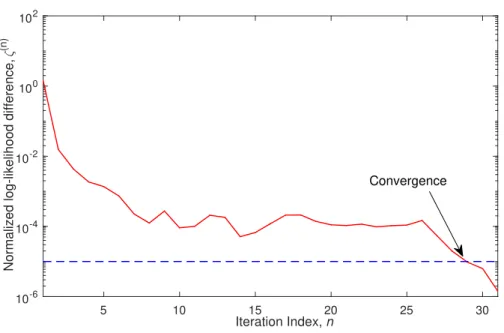
2.4 Normalized log-likelihood difference ζ(n) vs. SSEM iteration index, for (K, W) = (9,100). . . 29
2.5 (a) HSI used in the GRSS DASE [88] subpixel target detection experiment, (b) SSEM segmentation result (K = 9, W = 0), and (c) SSEM segmentation result (K= 16, W = 60).. . . 30
2.6 (a) HyMap image with 25 synthetic V1 targets and (b) V1 target signature. 31
2.7 PD vs. PFA for HyMap experiment. . . 32
2.8 PD and PFA confidence regions of SSEM and ACE ROC curves. . . 33
2.9 HyMAP image with simpler background and 25 implanted V1 targets (mag-nified location markers). . . 34
2.10 PD vs. PFA performance of compared detectors. . . 34
3.1 The overall framework of tree matching object detection algorithms. . . 39
3.2 The generation of the payoff matrix. . . 45
3.3 Tree matching on synthetic images: (a) Tree structure for target image. (b) First level match based on shape. (c) Tree structure for scene image. (d) Second level match result. . . 49
3.4 (a): Tree Structures for the object. (b) - (e): Regions corresponding to nodes 1,2,3,4 of the object tree. (f): First level matches of template root to the image tree. (g)-(i) Second level matches corresponding to node 2, 3, 4 of the object tree. . . 51
3.5 Scale tree overlaid on scene and template images. . . 52
3.6 Variations of the strategies and payoff during first run of game dynamics. . 54
3.7 Object detected after the first and fifth run of the algorithm. . . 55
3.8 Scale trees of HR remotely sensed images overlaid on scene and template images. . . 56
3.9 Object Detection in HR remotely sensed images. . . 57
4.1 Overall framework of the proposed approach. . . 62
4.2 Generation of the BoW image representations . . . 63
4.3 Examples of object and non-object image patches cropped from the LULC dataset [18] for training a “plane” detector . . . 68
4.4 Cross-validation experiments: the ROC curves for different classification algorithms using BoW descriptors based on SIFT (top) and SURF features (bottom). . . 70
4.5 Detection results with trained classifiers using LR (top), SVM (middle), and GP with LP approximation (bottom). Green: true positive; Blue: missed objects; Red: false positives . . . 72
5.1 The proposed scale transferrable detection network (STDN) for object de-tection in high resolution aerial images. . . 77
5.2 Proposed STDN with Inception v3 model as the base network. . . 78
5.3 Inception module with dimensionality reduction introduced in [148]. . . 80
5.4 An example of the Munich vehicle detection dataset. The image was cropped into small regions for training and testing. . . 85
5.5 Original rotated bounding box annotation (left) and transformed rectangle bounding box used (right). . . 87
5.6 Speed vs Accuracy comparison between Faster RCNN, SSD, and the STDN (proposed), with Inception v2 and Inception v3 as base networks. . . 91
5.7 Examples of Inception v2 based object detection, using different architec-tures: Faster R-CNN (first column), SSD (second column), proposed STDN approach (third column). . . 93
5.8 Precision recall curves of different detection algorithms, with Inception v2 as the base network. . . 94
5.9 Precision recall curves of different detection algorithms, with Inception v3 as the base network. . . 95
5.10 Precision recall curves of different STDN approaches, with DensNet and Inception v2/v3 as the base network. . . 96
2.1 DASE performance: 100×AUC (%), for PFA from 0 to 0.1 [89]. . . 30
4.1 Cross-validation experiments: performance comparisons on different classi-fiers for “plane” object detection. . . 69
5.1 Detail architecture with scale transfer module and backbone network of Inception v3 [149]. . . 82
5.2 Munich vehicle detection dataset statistics . . . 86
5.3 Average precision and inference time for different detection algorithms, with Inception v2 as base network. . . 92
5.4 Average precision and inference time for different detection algorithms, with Inception v3 as base network. . . 92
5.5 The effect of the scale transfer module in the proposed STDN approach. . . 97
Introduction
With rapid developments of remote sensing technologies, the availability of remotely sensed
images has expanded significantly in the past few decades. In order to obtain a complete
understanding of these images, it is crucial for the image analysts to learn whether the
ob-jects of interest are contained inside. As a result, object detection has been a fundamental
problem that plays an import role in many applications, such as geographical mapping [1],
urban planning [2], vehicle tracking [3], and environmental monitoring [4]. In this work, we
investigate frameworks and methodologies related to various object detection tasks in the
remote sensing field. Specifically, we make efforts to address the subpixel target detection
problem in hyperspectral images and explore the approaches related to geospatial object
detection in high resolution aerial images.
1.1
Problem Statements and Challenges
Given the large amounts of remote sensing images, it is implausible for the imaging
ex-perts to manually scan through the image data and look for the desired targets. Hence,
developing automatic detection algorithms is always an indispensable way. Over the past
few decades, object detection has driven a lot of research interests. However, it is still a
challenging task in hyperspectral images and high resolution aerial images even though
tremendous progresses have been made.
First of all, the objects of interest generally have unique appearances between different
image modalities and the approaches that deal with the detection problems are very
dif-ferent. In hyperspectral images, the target detection algorithms mainly focus on matching
the spectral signatures of image pixels given that of a target being sought after [3]. For
example, the well-known Airborne Visible InfraRed Imaging Spectrometer (AVIRIS) [5]
is able to generate hyperspectral images that cover the spectrum between 400 to 2500
nanometers with 224 continuous spectral bands. However, since the hyperspectral images
are usually obtained with low spatial resolutions [3], the observed spectral signatures of
image pixels are a combination of the target and the background spectrum. Therefore,
it is necessary for developing algorithms that suppress background inference by taking
additional spatial information. On the contrary, the approaches for object detection in
high resolution aerial images are quite different. For example, the World View-2 satellite
sensor [6], being targeted as the first high resolution multispectral commercial satellite,
is able to capture panchromatic images with the spatial resolution less than 0.5 meters.
With such a high spatial resolution, the obtained aerial images are able to capture
delineated. In this case, many techniques from the computer vision and machine learning
fields were adopted to identify the geospatial objects, including cars, ships, and building
structures.
Next, another challenging issue that amounts to the detection difficulties refers to the
intra-variations of the object appearances. For instance, the differences between the
spec-tral signatures of the observed targets in hyperspecspec-tral images result from unpredictable
sensor noises and artifacts, as well as the changing illumination conditions when the
hy-perspectral images are captured [7]. Similarly, the object variations in high resolution
aerial images usually include, but not limited to, object orientations, object occlusions,
and object scales [8,9]. In order to take into account of all these variations, it is important
to resort to some a-priori information when designing the detection algorithms. However,
it is nontrivial to develop an algorithm that has a powerful generalization capability for
all types of object variations.
Last but not least, the increased complexities of the image background make the design
of robust object detection algorithms more challenging. In hyperspectral images, each pixel
may contain a large portion of background regions, which suppresses the signature of the
target being searched for [10]. In high resolution aerial images, the vehicles may have the
appearance similar to that of the rooftops, which may lead to an increasing amount of false
positives in the final detection results. Distinguishing between them involves designing
algorithms that account for other information, such as the contextual knowledge [11]. As
a rule of thumb, it is critical to consider sufficient image background variations when
Figure 1.1: Overview of the research work in hyperspectral images and high resolution aerial images.
1.2
Research Goals
The purpose of this work is to develop object detection algorithms and frameworks that
better address the challenges discussed in the previous section. To this end, we approach
the detection problems in two image modalities: hyperspectral images and high resolution
aerial images. In Fig.1.1, a brief overview of the work in these two image domains was
presented.
In the first part of the thesis, we focus on the subject of detecting supbixel targets,
whose size is not spatially resolved in hyperspectral images. Given the target spectral
signature, the matched filter is the most widely used algorithm for hyperspectral
estimated from the hyperspectral images [13], with the underlying assumption that the
spectrum of background regions can be modeled as a single multivariate Gaussian
distribu-tion. In this regard, we study the effect of background modeling in designing the matched
filters. We proposed a novel image segmentation algorithm that divides the hyperspectral
image into spaio-spectral coherent regions. After that, the matched filters were applied
on the segmentation regions for subpixel target detection.
When dealing with high resolution aerial images, two detection frameworks, the object
based image analysis (OBIA) approach [14] and the machine learning based method, are
being investigated. In the OBIA approach, the aerial images are first divided into coherent
regions using segmentation algorithms. Motivated by the rich region descriptive features
[15], we extend the OBIA approach to generate hierarchical tree structures for the image
representation [16]. Our assumption is that the hierarchical tree structure is an improved
image representation for the object detection task, given its robustness to several image
deformations, such as scaling and rotation. Once the images are represented as tree
structures, the object detection problem is reformulated into a tree-matching task. We
then develop two tree matching algorithms for object detection.
The traditional machine learning based object detection framework converts the
de-tection problem into a classification task, which consists of the procedures of feature
ex-traction and classifier training. Feature exex-traction aims at achieving image feature vectors
that are invariant to different image variations. To this end, many image features
devel-oped in the computer vision field are extended to remote sensing, and have proved to be
effective and efficient for aerial image recognition. These include hand-craft features, such
as histogram of gradient (HoG) [17], bag of visual words (BoW) [18], GIST [19], and also
neural networks [21]. The second building block of the traditional machine learning based
approach involves training an object detector with classification algorithms. In our work,
we proposed to apply Gaussian process (GP) classification [22] for the detection task. We
demonstrate that the GP classifier is competitive to support vector machine (SVM) [23],
which was considered state-of-the-art in hand-craft feature based detection framework.
With rapid developments in deep learning techniques in recent years, various network
structures have been developed and powerful features have been learned from a large
amount of labeled data [24]. Object detection in the computer vision field has also changed
dramatically and different types of CNNs have been proposed for the detection task.
These networks vary in the design of architectures, the composition of object proposal
generations, as well as the schemes for optimization [25, 26, 27]. To better address the
small object detection problem in aerial images, a novel scale transfer module was proposed
to generate improved feature maps for object detection, leading to a detection framework
with both improved detection speed and high detection performance.
1.3
Contributions
The main contributions of the research work include:
1. Subpixel target detection
• Investigate segmentation based matched filters for subpixel target detection in
hyperspectral images.
• Propose a novel spatial-spectral image segmentation algorithm that produces
spatial-spectral coherent regions, where the background statistics were derived
• Attain the state-of-the-art subpixel target detection performance on the SHARE
2012 dataset [28].
2. Tree matching based object detection
• Propose an innovative object detection framework that represents the image
using a tree structure and reformulates object detection into a tree matching
problem.
• Apply graph theory and develop two novel tree matching algorithms to
effi-ciently detect geospatial objects in high resolution aerial images.
3. Machine learning based object detection
• In the traditional object detection framework, we present a detector using
prob-abilistic classification algorithms. When only a limited amount of training data
is available, we achieve the state-of-the-art performance comparing to other
popular object detectors.
• We investigate state-of-the-art CNN methodologies for geospatial object
de-tection. In particular, we apply a novel scale transfer module to effectively
generate the improved feature maps that facilitate small object detection in
high resolution aerial images.
1.3.1 Publications
We have presented the proposed target detection algorithms for hyperspectral images and
Journal articles:
1. Y. Liang, P. P. Markopoulos, and E. Saber, “Object detection in high-resolution
aerial images with scale transfer module”, under submission.
2. Y. Liang, P. P. Markopoulos, and E. Saber, “Novel spatial-spectral segmentation
of hyperspectral images for subpixel target detection”, SPIE Journal of Applied
Remote Sensing, 2019.
Conference papers:
1. Y. Liang, S. T. Monteiro, and E. Saber, “Gaussian processes for object detection in
high resolution remote sensing images”, IEEE International Conference on Machine
Learning and Applications, Anaheim, CA, December 2016.
2. Y. Liang, S. T. Monteiro, and E. Saber, “Transfer learning for high resolution aerial
image classification”, IEEE Applied Imagery Pattern Recognition Workshop,
Wash-ington D.C., October 2016.
3. Y. Liang, P. P. Markopoulos, and E. Saber, “Subpixel target detection in
hyperspec-tral images with local matched filtering in SLIC superpixels”, IEEE Workshop on
Hyperspectral Image and Signal Processing: Evolutions in Remote Sensing (IEEE
WHISPERS), Los Angeles, CA, August 2016.
4. Y. Liang, P. P. Markopoulos, and E. Saber, “Subpixel target detection in
hyperspec-tral images from superpixel background statistics”, IEEE International Geoscience
and Remote Sensing Symposium, Beijing, China, July 2016.
5. Y. Liang, N. D. Cahill, and E. Saber, and D. W. Messinger, “A game-theoretic tree
SPIE Proceedings: Image and Signal Processing for Remote Sensing XXI, Toulouse,
France, September 2015.
6. Y. Liang, A. H. Syed, N. D. Cahill, E. Saber, and D. W. Messinger, “Application of
tree matching techniques to high resolution remotely sensed images toward object
detection”, Geographic Object-Based Image Analysis, Thessaloniki, Greece, May
2014.
1.4
Thesis Organization
The remainder of the thesis is organized as follows. In the first part, we present our
work on subpixel object detection in hyperspectral images in Chapter 2. In the second
part, we describe our algorithms for object detection in high resolution aerial images with
three chapters. In Chapter 3, the tree matching based object detection algorithms are
discussed. Following that, we focus on the Gaussian process classifier for object detection
in Chapter4. We then present our work on deep learning based approach in Chapter 5,
where a novel scale transfer module is proposed. Finally, in Chapter 6, we summarize
the observations and conclusions from the experimental studies for both subpixel target
detection in hyperspectral images and geospatial object detection in high resolution aerial
Subpixel Object Detection
In this chapter, we study the subpixel target detection problem in hyperspectral images,
where the subpixel target refers to the objects with spatial size less than the spatial
res-olution of the image pixel. Previously, we have explored the segmentation based subpixel
target detection framework and presented our initial results using the SLIC algorithm
[29,30]. Recently, we extend the detection framework with a novel spatial-spectral image
segmentation approach and our results have been published in [31]. The content of this
chapter is organized as follows. In the Section2.1, the subpixel target detection problem
are introduced. In the Section2.2, we point out the importance of background modeling for
designing the matched filter and review the previous work on the topic. Following that, we
present our detection framework in Secion2.3, which includes the spatial-spectral
expecta-tion maximizaexpecta-tion image segmentaexpecta-tion algorithm and region-based matched filter design.
Finally, we present our detection performance with both synthetic target-implantation
experiments and SHARE 2012 subpixel target detection task in Section 2.4. Our results
demonstrate the superiority of our proposed subpixel target detection framework.
2.1
Introduction
The problem of subpixel target detection in Hyperspectral Images (HSI) has attracted
extended research interest in the field of remote sensing, due to its many important civil,
military, and environmental applications. Such applications include, among others,
min-eral detection for geology exploration [32], crop identification for agriculture monitoring
[4], military vehicle tracking for security and defense [3], and detection of uranium for
nuclear threat identification [33].
Existing algorithms for subpixel target detection in HSI consider several different
mod-els for the reflectance spectrum of a target-containing pixel [34, 10, 35]. Arguably, the
most widely adopted model is the Linear Mixing Model (LMM) [10, 36], according to
which the spectrum of a pixel is represented by linear combination of the target signature
with multiple background endmembers. In LMM, the background endmembers constitute
additive interference with respect to the target spectrum [37]. In their seminal work [10],
Manolakis et al. derived the popular Generalized Likelihood Ratio Test (GLRT) detector
for LMM. In GLRT, the per-pixel target detection problem is formulated as a test between
two competing hypotheses of target-presence and target-absence. An additional constraint
on the fixed detector response of the target signature has lead to the Constrained Energy
Minimization (CEM) detector [34]. Other popular detectors include the Orthogonal
Sub-space Projection (OSP) detector [38], the Spectral Matched Filter (SMF) detector [32],
and the Adaptive Cosine Estimator (ACE) detector [39], where ACE and SMF are defined
upon the unstructured background assumption. In addition, detectors based on spectral
similarities have also been proposed, such as the Spectral Angle Mapper (SAM) [40].
For example, OSP and CEM were compared with ACE in [41] using the standard Target
Implant Method (TIM). Similarly, SMF, ACE, and SAM were compared on various types
of hyperspectral images, captured with different sensor modalities [35,42].
For the sake of completeness, it is worth noting that, apart from the popular
LMM-based detectors discussed above, several target detection methods LMM-based on statistical
signal processing and machine learning techniques have also been explored [43, 4,44, 45,
46] in the past. For instance, detectors based on subspace as well as physical models were
explored in [43] for hyperspectral target detection. The authors in [44] used a kernel-based
approach to derive non-linear equivalents of LMM-based detectors. In addition, subpixel
target detection has also been studied as a binary classification task [45] with no prior
distribution assumptions on the HSI. However, such data-driven methods usually require
a large number of training samples from both classes (target-absence and target-presence),
which are often difficult to collect.
Recent studies have indicated that identifying statistically coherent image regions can
result in local detectors with improved performance [13, 7, 47]. By the term “coherent
region” we refer to a part of the HSI within which all (background) pixels can be
statisti-cally described by a single mean-vector/covariance-matrix pair. Segmentation techniques
have also been applied before for both anomaly [48, 49, 50] and change detection [49].
While spectral clustering by means of K-means is widely used for image segmentation
[49,51,48], other approaches have also been proposed. These approaches include
graph-based methods [52, 53], stochastic EM [54], sparse representations [55], clustering based
on non-Gaussian models [56], segmentation based on spatial-spectral information [57], and
segmentation based on band selection [58]. In that direction, for subpixel target detection,
where K-means clustering was employed in the spectral domain for hyperspectral image
segmentation and local matched filtering. In addition, Cohen et al. improved the GLRT
detectors by replacing the “global” mean vector with a “locally” calculated counterpart
[59,60]. Importantly, the recent work of Rotman et al. in [61, 62] showed that
spectral-segmentation-based target detectors can attain significantly improved performance, when
the segment covariance matrices are sufficiently different.
In this work, we introduce the Spatial-Spectral Expectation-Maximization (SSEM)
algorithm for HSI segmentation in both spatially and spectrally coherent regions and
subpixel target detection therein with local matched filters. Our experimental studies on
both real and synthetic data corroborate the benefits of the proposed method, especially in
the case of complex image backgrounds, and compare it with state-of-the-art counterparts.
2.2
Problem Statement and Background
2.2.1 Image Model
We consider HSI X ∈ RR×C×L that contains N = RC pixels and L spectral bands. In
accordance to the standard Linear Mixing Model (LMM) [10], we express the spectrum
xi of a single pixel in the image as:
xi ,aisT+
P
X
p=1
ap,isp+wi ∈RL×1, (2.1)
wheresT ∈RL×1 is the target signature, sp is the signature of the p-th background
end-member, and ai, ap,i are the corresponding “fill-factors”, taking values in [0,1] so that
modeled and measured spectra and follows zero-mean and white Gaussian distribution.
According to (2.1), when ai <1, the target spectrum is mixed with background
compo-nents within xi and, thus, the target is referred to as “subpixel” target. In this work,
our focus lies on developing a systematic method for determining whether xi contains
the subpixel target or not (target detection), for every i ∈ {1,2, . . . , N}. Denoting the
aggregate background-plus-noise component inxi by:
di , P
X
p=1
ap,isp+wi, (2.2)
we can then re-write (2.1) in the familiar form [32]:
xi=aisT+di. (2.3)
Certainly, if thei-th captured pixel contains the subpixel target, thenai >0; conversely,
if xi contains only background-plus-noise, then ai = 0 and xi = di. When ai takes low
values in (2.3), target presence is weak and the background-plus-noise component inhibits
target detection. For simplicity in presentation, we henceforth consider constant target
fill factorai∈ {0, a}, for somea >0 –i.e., all instances of the subpixel target take up the
same space in their corresponding pixels.
2.2.2 Standard Global Matched-Filter
Considering deterministic sT and randomdi drawn from multivariate Gaussian
distribu-tion with meanm ∈ RL×1 and covariance matrix C∈
(LRT) onxi develops into the popular matched filter (MF) detector [32,47] yMF(xi),wTMF(xi−m) target present ≥ < target absentη, (2.4)
where η is the LRT decision threshold and wMF , C −1(s
T−m) √
(sT−m)TC−1(sT−m)
. Certainly, the
background-plus-noise distribution statisticsmandCare a priori unknown to the detector
and have to be estimated from the given imageX. Traditionally,mand Care estimated
on the entire image (“global” statistics [13]) as:
ˆ mG, 1 N N X i=1 xi, and CˆG, 1 N N X i=1 (xi−mˆG)(xi−mˆG)T, (2.5)
respectively. The correspondingly derived “global” estimate of the matched filter (GMF)
takes the form: [32,13]
wGMF , ˆ C−G1(sT−mˆG) q (sT−mˆG)TCˆG−1(sT−mˆG) (2.6)
and the MF detector in (2.4) practically operates onyGMF(xi),wTGMF(xi−mˆG), instead
ofyMF(xi).
We notice that estimation of background statistics over both background-only and
target-bearing pixels (in lieu of discerning knowledge at this point) is a common practice
when the number of pixelsN in the image is large and only few of the pixels host targets,
with low filling factorai [32]. The above standard GMF detector has been extensively used
in the HSI literature, due to its simplicity in calculation and high performance when the
suffices for describing the background content of every pixel in the HSI and, thus, can be
estimated thereof.
2.2.3 Motivation of Local Matched Filter
At this point, to motivate the methodology proposed in this paper, it is worth considering
the above presented MF detector from a linear processing viewpoint. As shown above,
the matched filter aims at suppressing the background component in xi by whitening its
covariance matrix and, subsequently, reveals target presence by match-correlating with the
mean-centered target signature. Certainly, when the image contains uniformly coherent
background regions, this task can be successfully accomplished by filtering all pixels in the
image with the same MF,wGMF, defined upon the global estimates ( ˆmG,CˆG). However,
in many cases of practical interest, the statistical description of the background may
vary, possibly significantly, throughout the pixels of the HSI. In such cases, the single,
globally estimated, pair of background statistics ( ˆmG,CˆG) is expected to under-perform
in statistically representing some, or even all, of the diverse background components in
the image.
To address this common problem, in this work we consider that the HSI can be
natu-rally segmented/clustered in multiple regions of statistically coherent background. Thus,
we first steer our focus on identifying these coherence regions. Then, we focus on
estimat-ing and employestimat-ing local background statistics for target detection. That is, we test pixel
xi for target content by means of a MF that is defined upon background statistics of the
background-coherence region wherein xi belongs.
The positive impact of locally calculated background statistics in MF-based target
Pieper et al. in [47] proposed a method for estimating local background statistics by means
of combining sliding window and image segmentation. Funk et al. in [51] applied K-means
to cluster the target-hosting HSI and then applied individual local matched filters in each
cluster. Similarly, Rotman et al. in [63,64] calculated local matched filters from
spectral-coherence regions obtained through histogram clustering [65, 66]. Extending the above
results, in this work we notice that EM is, arguably, the clustering approach that would
most naturally capture statistical spectral coherence within distinct image regions [67,68,
69, 70]. Understandably, if one clusters pixels based only on their spectral content, it is
expected that, for sufficiently high fill-factor, most target-bearing pixels may be assigned
to the same cluster, together with other similar background-only pixels (unbeknown to the
target detector). This would clearly inhibit significantly background suppression within
this target-loaded cluster and, thus, target detection overall. To regulate cluster formation
so that spatial locality is naturally preserved and avoid the formation of the heavily
target-loaded clusters, we also consider a regularization factor that promotes spatial coherence in
the formed clusters. In addition, a diagonal loading term [71,72,73,74,75] is incorporated
to guarantee that the estimated background covariance matrix is invertible. Therefore, the
resulting image segmentation regions preserve the pixel locality and group a target-bearing
pixel together with its background-coherent neighbours – thus, allowing us to process it
by a MF built on relevant background statistics. The proposed target detection scheme is
Figure 2.1: Overview of proposed SSEM method for subpixel target detection.
2.3
Proposed Method
As illustrated in Fig. 2.1, first we apply the proposed SSEM algorithm to segment the
target-hosting HSI into non-overlapping spatial-spectral coherence regions. Then, for each
coherence region, we derive and apply the corresponding local matched filter to detect
target presence.
2.3.1 Proposed Spatial-Spectral Image Segmentation
We commence with the instrumental assumption that there exists a size-K group of
Gaussian distributions,N(m1,C1), . . . ,N(mK,CK), such that, for every i∈ {1, . . . , N},
di ∼ N(mk,Ck), for some k ∈ {1,2, . . . , K}. Certainly, the more spectrally-diverse the
HSI at hand, the higher the number of distributions,K, that are needed to model its
back-ground. In this first part of our scheme, we aim at identifying for everyk∈ {1,2, . . . , K}
the region-index setIk⊆ {1,2, . . . , N}, such thatdi∼ N(mk,Ck) for everyi∈ Ik. That
is,Ik holds the indices of the pixels that constitute thek-th background-coherence region
of the HSI, Xk ={xi; i∈ Ik}. Then, we use the pixels in Xk to estimate the local
back-ground statistics mk and Ck and, accordingly, the corresponding local MF detector. To
identify{Ik}K
k=1, we introduce the SSEM segmentation algorithm presented below.
Dimensionality Reduction: SSEM starts with matricizing the HSI data to define
each image pixel. Then, to expedite segmentation, we approximateXby the low-rank ˜X,
U>X∈RD×N,where D≤L andU∈
RL×D is the matrix that contains the Ddominant
left-singular vectors of X, obtained by means of standard Singular Value Decomposition
(SVD) [76] or, alternatively, L1-PCA [77,78]. The underlying notion is that, if the
low-rank approximation normalized error e(D;X) , kXk
2 F−kU >Xk2 F kXk2 F
is small,1 then we can
obtain the coherence regions in the original imageX by segmenting the low-rank ˜X with
significantly reduced computational workload, as discussed below. Accordingly, it holds
that ˜xi ,UTxi =aUTsT+UTdi =a˜sT+ ˜di, where ˜sT ,UTsT, and ˜di ,UTdi is drawn
fromN(UTmk,UTCkU), for everyi∈ Ik.
Initialization: Next, we initializeKregion-index sets{Ik(0)}K
k=1 defined, for example,
byK non-overlapping rectangular tiles that cover the entire HSI. GivenK and the image
dimensions, we choose the initial tiles so that the region size|Ik|varies minimally across
k∈ {1,2, . . . , K}. Accordingly, we initialize the prior probability of thek-th region as:
π(0)k = |I
(0)
k |
N (2.7)
where| · |returns the number of distinct elements (cardinality) of its set argument. Next,
for every i∈ {1,2, . . . , N}and k∈ {1,2, . . . , K}, we set the probability that di is drawn
from the k-th coherence region at the initial value:
p(0)i,k = 1, ifi∈ Ik(0) 0, otherwise . (2.8)
1In the approximation error,k·k2
F denotes the squared Frobenius norm returning the sum of the squared singular values of its matrix argument [76].
After initialization, SSEM proceeds iteratively as follows.
Iterations: Each iteration consists of an expectation and a maximization step (EM
iterations). At then-th expectation step, we calculate theregion-membershipprobabilities:
γk,i(n)= p (n−1) i,k π (n−1) k PK l=1p (n−1) i,l π (n−1) l (2.9)
for every region k∈ {1,2, . . . , K} and pixel index i∈ {1,2, . . . , N}. Then, at the
subse-quentn-th maximization step, we first update the index set
Ik(n) = n i∈ {1,2, . . . , N}:k= arg max l∈{1,...,K} γl,i(n) o (2.10)
for everyk∈ {1,2, . . . , K}. Accordingly, for every k∈ {1,2, . . . , K}, we update the prior
πk(n) = PN i=1γ (n) k,i PK l=1 PN i=1γ (n) l,i (2.11)
and adapt the region statistics as:
m(kn) = 1 PN i=1γ (n) k,i N X i=1 γk,i(n)x˜i and (2.12) C(kn) = 1 PN i=1γ (n) k,i N X i=1 γk,i(n)(˜xi−mk(n))(˜xi−m(kn)) T. (2.13)
Finally, for everyi∈ {1,2, . . . , N}and k∈ {1,2, . . . , K}, we update the likelihood of the
k-th region, in view of ˜xi, as:
p(i,kn)= (2π)L|Ck| −12 exp ( − 1 2DSpectral(i, k)−W DSpatial(i, k) ) , (2.14)
considering both the spectral and spatial squared distances ofxi to thek-th region: Dspectral(i, k) = (˜xi−mk(n))T(Ck(n))−1(˜xi−m(kn)), (2.15) Dspatial(i, k) = 1 dkci−z (n) k k 2. (2.16)
In (2.16),ci is the vector that contains the spatial coordinates of thei-th pixel in the HSI,
so that c1 = [1,1]>, c2 = [2,1]>, . . .cR+1 = [1,2]>, . . . , cN = [R, C]>. z(kn) is the spatial
“centroid” of thek-th cluster, calculated as:
zk , 1 |Ik(n)| X i∈Ik(n) ci. (2.17)
Finally,d,(R−1)2+ (C−1)2 is a normalizing factor so that kc1−cNk2 = 1 and, thus,
Dspatial(i, k)≤1.
In our algorithm, the number of regionsK for image segmentation is determined from
the complexity of the image background; i.e., the more complex the image background is,
the larger the value ofK that we choose. In (2.14),W is a positive spatial regularization
parameter that wishes to restrain spatially the segmentation, ameliorating the impact of
possible target content in ˜xi. That is, the spatial penalty (distance) Dspatial(i, k) aims at
preventing the formation of spectral-only coherence regions that are heavily target loaded
and in which it would be infeasible to calculate background statistics for successful
back-ground whitening and target detection. Instead, by means of this spatial regularization,
target-bearing pixels are clustered together with their background-coherent neighbors and,
thus, are processed for target detection by MF built on the relevant background statistics.
be-tween spectral and spatial proximity of HSI pixels has also been proposed in other recent
works such as in [79] for image classification and [80] for HSI restoration.
The above presented SSEM iterations continue until convergence is met, as discussed
below. Of course, in practice, the iterations can be terminated earlier than convergence
for complexity savings. Upon termination at iteration n, SSEM returns the cluster
mem-bership index sets {Ik=Ik(n)}Kk=1.
Convergence: In this work, we have refrained from re-deriving the EM iterations from
their statistical optimality grounds, as they constitute a broadly familiar and extensively
employed clustering method [81,82,83]. However, for completeness, we find it appropriate
to provide below few words on their convergence. The aggregate log-likelihood of the HSI
at then-th iteration step is defined as:
l(n), N X i=1 K X k=1
γk,i(n)log(pi,k(n)π(kn)). (2.18)
By their definition, the priors in (2.11), membership probabilities in (2.9), parameters in
(2.12)-(2.13), and likelihood in (2.14), are defined to maximize alternatingly (2.18). The
monotonic increase of the l(n), throughout the iterations, guarantees their convergence
[81]. The proposed SSEM segmentation is summarized in Algorithm 1.
2.3.2 Proposed Local MF in SSEM Regions
When the coherence-region identification completes, the background statistics are
esti-mated from the pixels of each coherence region and employed to form the corresponding
local matched filters. Specifically, we estimate the background mean and covariance
Algorithm 1 Proposed SSEM segmentation algorithm.
Proposed SSEM image segmentation Input: X,K,W,D≤L Initialization: Ik(0),π(0)k ← |I (0) k | N , p (0) i,k ← ( 1, ifi∈ Ik(0). 0, otherwise.,n←0 Dimensionality Reduction: U∈RL×D←svd(X), X˜ ←U>X
Until termination is met, don←n+ 1
Expectation: for (i, k)∈ {1, . . . , N} × {1, . . . , K} γk,i(n)← p (n−1) i,k π (n−1) k PK l=1p (n−1) i,l π (n−1) l end Maximization: fork∈ {1, . . . , K} Ik(n)←ni∈ {1,2, . . . , N}:k= arg maxl∈{1,...,K} γ (n) l,i o πk(n)← PN i=1γ (n) k,i PK l=1 PN i=1γ (n) l,i m(kn)← 1 PN i=1γ (n) k,i PN i=1γ (n) k,i˜xi C(kn)← 1 PN i=1γ (n) k,i PN i=1γ (n) k,i(˜xi−m (n) k )(˜xi−m (n) k ) T p(i,kn)= (2π)L|C k| −12exp ( −1 2DSpectral(i, k)−W DSpatial(i, k) ) end Output: {Ik← I (n) k } K k=1
Algorithm 2 Target detection by SSEM-based local matched-filtering.
Proposed SSEM-based target detection Input from Algorithm 1: {Ik}Kk=1,λ, η fork∈ {1, . . . , K} ˆ mk← |I1 k| P i∈Ikxi ˆ Ck ←|I1 k| P i∈Ik(xi−mˆk)(xi−mˆk) T +λI wMF,k ←Cˆ−k1(sT−mˆk)((sT−mˆk)TCˆk−1(sT−mˆk))− 1 2 fori∈ Ik
Detect target presence inxi, ifwTMF,k(xi−mˆk)> η
end end
as: ˆ mk= 1 |Ik| X i∈Ik xi and Cˆk= 1 |Ik| X i∈Ik (xi−mˆk)(xi−mˆk)T +λI, (2.19)
respectively.2 In (2.19), λ > 0 is a low-valued regularizer for diagonal loading and I is
the size-Lidentity matrix. Many methods for optimum, or preferred selection of diagonal
loading factor have been presented in the area of adaptive filtering/beamforming; for
example, we refer the interested reader to the works in [73, 74]. By the diagonal loading
λI, it is guaranteed that, even for small coherence regions, the estimated covariance matrix
will be of full rank and, thus, invertible [71,72,73,74,75]. Based on the above estimated
statistics, the matched filter for thek-th region is formed as:
wMF,k = ˆ C−k1(sT−mˆk) q (sT−mˆk)TCˆk−1(sT−mˆk) . (2.20)
Then, for everyxi withi∈ Ik, the target presence/absence is tested locally as:
yMF,k(xi) =wMFT ,k(xi−mˆk)
target present
≥ <
target absentη. (2.21)
The proposed SSEM-based target detection is summarized in Algorithm2.
2.3.3 Computational Complexity
Understanding that the computational cost of segmentation-based target detectors is
of-ten a concern, at this point we discuss the complexity of the proposed scheme. The
2
Note that matched filtering takes place inRD
, and not in the reduced rank segmentation subspace
span(U), where the targets may be suppressed. Dimensionality reduction is only used at the segmentation step.
proposed detector involves SSEM segmentation, local background statistics estimation,
MF calculation, and application for target detection. In SSEM segmentation,
initializa-tion costs O(N L2) for reducing the dimensionality of X, assuming that L ≤ N (more
image pixels than spectral bands), andO(N K) for setting initial values to {πk(0)}K k=1 and {p(0)i,k}K
k=1. Then, calculation of (2.9), (2.10), and (2.11), for everyk ∈ {1,2, . . . , K} and
everyi∈ {1,2, . . . , N}, costsO(N K), per iteration. Updating the K statistics in (2.12
)-(2.13) costsO(N KD2). Calculating all covariance-matrix inverses for (2.15) costsO(KD3)
–we note that this cost would beO(KL3), cubic in the number of frequency bands, if we
did not perform segmentation on the reduced image dimensions. Then, (2.14)-(2.16) cost
an additional O(N KD2). Thus, the computational cost of each iteration can be
sum-marized as O(N KD2). Considering termination (as indicated by our numerical studies)
after a constant multiple ofKDiterations, the cost of SSEM segmentation is in the order
of O(N K2D3). Posterior to SSEM, the local MFs can be calculated and applied with
cost O(N KL2). Thus, the overall cost of the proposed target detector is linear to the
number of pixels,N, and quadratic to the number of frequency bands,L, and regions,K:
O(N KL2+N K2D3).
2.4
Experimental Studies
2.4.1 Experiment on SHARE 2012
For our first experimental study, we consider the SHARE 2012 [28,84] dataset. Here, the
HSI was obtained with the ProSpecTIR-VS sensor and the ground truth target locations
were calculated by means of a high resolution WASP sensor (1 sample per meter). The
Figure 2.2: (a) SpecTIR-VS sensor image with ground-truth target locations (green points) [28] and (b) the green wood panel hyperspectral signature.
open green grassy area. In accordance with the analysis of [85, 86], we operate on 50
spectral bands of the HSI, ranging from 418 nm to 643 nm. The test image, annotated
with ground-truth target locations, and the hyperspectral signature of the green wooden
panel are illustrated in Fig. 2.2. Considering the size of the wooden panels and the image
spatial resolution,3 it has been suggested that each target occupies a pixel in the image
with a fill-factor ranging from 5% to 20% [28].
First, SSEM partitions the HSI into spectral-spatial coherent regions. Then, local
matched filtering is applied per region for target detection. While automatic selection of
the number of regions/clusters is studied in the literature [87], in this work we simply
tuneK based on the complexity of the image; this relies on the simple (and numerically
validated) notion that images with complex background contain multiple coherent regions.
3
The fill-factor is defined as the ratio between the area covered by the panel target and the ground area of the image pixel.
The space-spectrum regularization parameter W is tuned so that a potentially high
fill-factor does not result in isolating target-bearing pixels from their coherent-background
neighbors. Thus, when the target size is expected to be large, with respect to the spatial
resolution of the HSI, we tune regularization W to higher values. Similar qualitative
(ad hoc) tuning of spatial-spectral regularization parameters has also been applied in the
recent literature for HSI classification and restoration [79,80], among other applications.
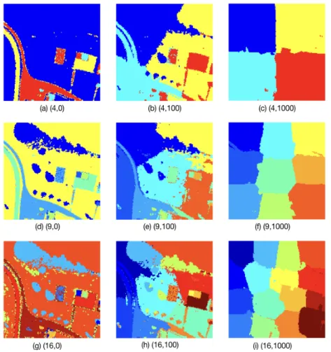
Instances of SSEM segmentation for different values ofK and W are presented in Fig.
2.3. We observe that variations of these parameters affect image segmentation results
significantly. When W = 0, SSEM clusters the image pixels based solely on their
spec-tral content. As W increases, spatial proximity is taken into consideration, resulting to
spatially coherent regions. In the extreme example of W = 1000, “gird-like” regions are
returned and the spectral content of the pixels is practically neglected.
Regarding the diagonal loading parameterλ, since its sole purpose is to guarantee that
the local covariance matrix is invertible, it suffices to set it significantly lower than the
minimum (non-zero) singular-value of the HSI matrix, as that is calculated during the
dimensionality reduction fromX to ˜X. In all our numerical studies, we setλ= 10−5.
Next, in Fig.2.4, we demonstrate the termination of the SSEM iterations by plotting
the the normalized log-likelihood differenceζ(n) , |l(n)|l(n−l−(n1)−|1)|, versus the iteration index, n. In this study, we have set K = 9 and W = 100. In practice, SSEM iterations are
hard-coded to terminate when the l(n) drops below an arbitrary low threshold, close to
0. In our studies, this threshold is set to 10−5. In the study of Fig. 2.4, the normalized
log-likelihood drops below that threshold at the 28-th iteration.
Next, we apply SSEM to the Avon 12 dataset [88], which also corresponds to a region
5 10 15 20 25 30 Iteration Index, n 10-6 10-4 10-2 100 102
Normalized log-likelihood difference,
(n)
Convergence
Figure 2.4: Normalized log-likelihood difference ζ(n) vs. SSEM iteration index, for (K, W) = (9,100).
225×360 and the subpixel targets are again the green wood panels. We operate on the
same spectral bands as before.
Applying the proposed detection algorithm (K = 16,W = 60), we generated the filter
response map and uploaded it to the Data and Algorithm Standard Evaluation (DASE)
website [89], which evaluated the performance of SSEM. The HSI of Avon12 together with
the obtained SSEM segmentation maps are illustrated in Fig. 2.5.
According to DASE, SSEM attained top score4 of 95.35% accuracy [89]. In Table
2.1, we present the performances of SSEM, GMF [32], AMF [3], CEM [34], ACE [39],
HIST [64], TVHTD [90], and K-means [51], as calculated by the DASE website. Table2.1
shows that all methods perform similarly well and demonstrates the merit of the proposed
4
In the assessment of DASE, the score is computed by measuring the AUC for PFA ranging between 0 and 0.1; this number is then multiplied by 10 and expressed as a percentage.
Table 2.1: DASE performance: 100×AUC (%), for PFA from 0 to 0.1 [89].
Figure 2.5: (a) HSI used in the GRSS DASE [88] subpixel target detection experiment, (b) SSEM segmentation result (K= 9, W = 0), and (c) SSEM segmentation result (K = 16, W = 60).
method.
2.4.2 HyMap Experiment
In this study, we consider synthetic target implantation. Similar other works in the recent
literature (e.g., [90]), we operate on a target-free image of the HyMap HSI [91] of small
size 100×100. Moreover, similar to [90], we removed spectral bands with more than
1000 negative values, as they correspond to water absorption and noisy bands with low
signal noise ratio (SNR) values. Then, we inserted 25 vehicle targets (V1), with fill-factors
varying betweena= 0.01 anda= 0.05. The small size and diverse background of the chose
Figure 2.6: (a) HyMap image with 25 synthetic V1 targets and (b) V1 target signature.
the image and the target locations (red dots).
In our experiments we did not normalize the target signature before inserting it to
the image. Specifically, the ratio of the squared norm of the target signature over the
average squared norm of the HSI pixels isγ , ksTk2 1 NkXk2F
= 419.22. If, instead, we consider
normalized target signature so thatγ = 1, then our setup corresponds to fill-factors ranging
fromαnorm= 0.2 to αnorm= 1.
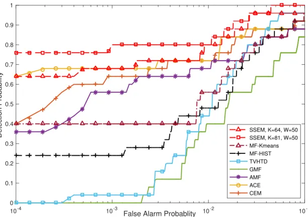
In Fig. 2.7, we plot the PD vs. PFA (0 to 0.1) performance of the proposed SSEM
(K = 81, W = 50), together with those of CEM, ACE, AMF, GMF, TVHTD, HIST and
the K-means based matched filter. For SSEM, K = 64 and K = 81 were tested, due to
the complexity of the image background. For K-means, K was set to 81. We observe
that SSEM and ACE attain top performance, with the proposed being somewhat superior
forK = 81. CEM and AMF closely follow, while GMF performs the exhibits the lowest
PD, almost for every value of PFA. We also notice that all methods tend to similar PD,
10-4 10-3 False Alarm Probablity 10-2 10-1 0 0.1 0.2 0.3 0.4 0.5 0.6 0.7 0.8 0.9 1
Detection Probability SSEM, K=64, W=50SSEM, K=81, W=50 MF-Kmeans MF-HIST TVHTD GMF AMF ACE CEM
Figure 2.8: PD and PFA confidence regions of SSEM and ACE ROC curves.
more background pixels would be needed.
In addition, for clarity, in Fig. 2.8, we plot the 95% confidence regions (PD and PFA)
[92] for SSEM (K= 81) and ACE.
Next, we carry out another experiment on a different part of the HyMap image, with
the same size as before, but simpler background (see Fig. 2.9). Similar to the previous
experiment, we implant 25 V1 targets with fixed target fill-factor ofa= 0.01 (oranorm=
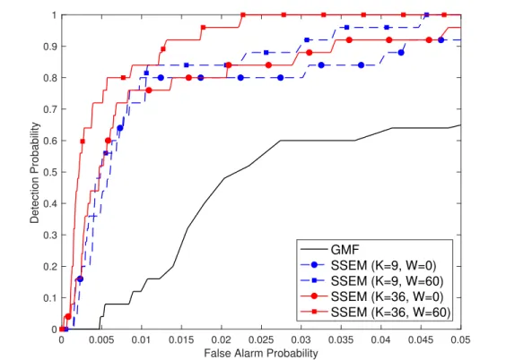
0.18). In Fig. 2.10, we plot the performance of SSEM for all combinations of K = 9, 36
andW = 0, 60, as well as that of the GMF benchmark. We notice that SSEM outperforms
MF for all the presented PFA values. Also, the figure demonstrates the effect of K and
Figure 2.9: HyMAP image with simpler background and 25 implanted V1 targets (mag-nified location markers).
0 0.005 0.01 0.015 0.02 0.025 0.03 0.035 0.04 0.045 0.05
False Alarm Probability
0 0.1 0.2 0.3 0.4 0.5 0.6 0.7 0.8 0.9 1 Detection Probability GMF SSEM (K=9, W=0) SSEM (K=9, W=60) SSEM (K=36, W=0) SSEM (K=36, W=60)
Tree Matching Approaches for
Object Detection
In this chapter, we apply the object based image analysis (OBIA) for object detection in
high resolution aerial images. Specifically, we develop methodologies to represent images
with tree structures and reformulate object detection into tree matching problems. We
then resort to graph theory and apply tree matching algorithms for our detection work.
This chapter is organized as follows. In Section 3.1, the background and motivation for
OBIA are discussed. We then proceed with the details of the proposed two tree matching
approaches for object detection in Section 3.2. Following that, we present the object
detection results in Section3.3 and Section3.4, where each tree matching algorithm was
applied to both synthetic images and high resolution aerial images. Our work has been
published in two conference papers, one based on tree association graph (TAG) [93] and
the other one based on the evolution game theory [94].
3.1
Introduction
The object based image analysis (OBIA) refers to the framework that analyzes images
based on the segmentation regions [14]. It is an object oriented approach for image analysis
[95], aiming at dealing with the complexities of the images. Ever since its emergence in
the remote sensing field, a large amount of progress has been witnessed in the past decades
for different applications, including damage analysis [96], disaster management [97], crop
and forest type identification [98], change detection [99], and urban land cover extraction
[100].
Before the emergence of OBIA in remote sensing, the pixel-based image analysis was
utilized. However, the pixel-based image analysis was found to be undesirable and there is
always a need to incorporate contextual information for the image analysis. For example,
the conventional pixel based image classification approaches tend out to be noisy [96]
and the object based approach overcomes this issue through combining the spectral and
spatial information. As a result, the salt-and-pepper noise found in pixel-based image
classification are substantially suppressed [101,102].
Generally, the OBIA framework involves image segmentation and object classification
[46]. The image segmentation procedure aims at partitioning the images into coherent
regions according to a certain homogeneity criteria and is the building block of the OBIA
method. It is expected that these individual homogeneous regions provide us with groups
of pixels with semantic contents [103]. Once the image is segmented, object candidate
regions are generated. The next step in this framework extracts, for each individual
region, the feature representations, which usually include spectral, size, shape, texture,
image regions.
To accommodate the image complexities, the multi-scale properties of the images have
also been studied based on the OBIA framework. Over the past decades, the multi-scale
image segmentation has been extensively studied for many applications, including urban
planning [104], object extraction [105], forest classification [106], geospatial object
detec-tion [107], and landscape analysis [108]. In these multi-scale analysis frameworks, the
bottom-up and top-down hierarchical image segmentation algorithms were applied to
ex-plore different scale space of the input image [109]. In addition, the spatial correlations
from these multi-scale segmentation regions were also studied. For example, the
hierarchi-cal shierarchi-cale structure of the multi-spectral image was proposed in [108], where a particular
scale domain was extracted for further analysis. Similarly, the structure information
be-tween multiple scales of the image segmentation was utilized to provide more intuitive and
accurate classification [107]. Furthermore, the spatial correlations between multi-scale
re-gions were represented as multi-scale region adjacency trees for hierarchical labeling [110].
Multi-scale image segmentation were found to be effective for geospatial object
extrac-tion. For instance, Akcay et. al. [107] construct hierarchical segmentation tree and design
a generic algorithm for selecting meaningful segments. Moreover, a multi-scale solution
based on mathematical morphology were developed in [104] for building extraction.
3.2
Tree Matching Algorithms for Object Detection
From discussions above, we notice that there is no single segmentation of an image that
is sufficient to capture all the available multi-level information for object detection. The
the optimum segmentation scale for specific classification task is identified [108]. In the
proposed framework, we investigate tree structures generated from these multi-scale image
segmentations and explore tree matching approaches for geospatial object detection.
Specifically, we employ multiple segmentations and resort to a scale tree structure [16]
for image representation, where each level of the scale tree denotes an image segmentation.
Different from the segmentation tree being built in a top-down way [111], our algorithm
builds the scale tree bottom-up through hierarchically merging segments. In the final
tree structure, the nodes represent image segmentation regions and the edges denote the
relative containment information between these regions at different scale levels. Given the
tree representations of a scene and the query object, the object detection is formulated
as a tree matching problem. In this section, we present two tree matching algorithms to
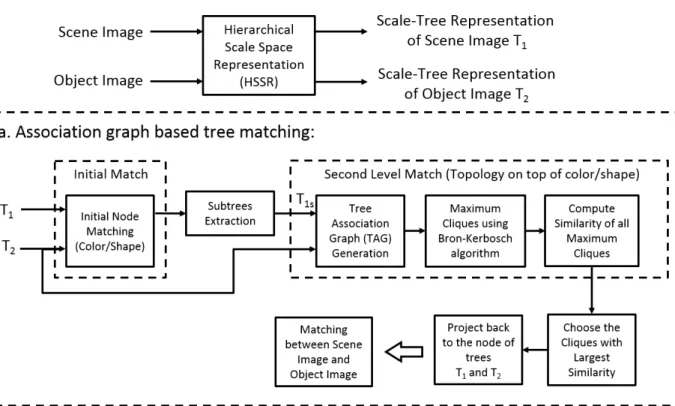
search for the query object within the scene image, as illustrated in Figure 3.1.
3.2.1 Association Graph based Tree Matching
The tree association graph (TAG) based tree matching is performed with the following
steps:
1. Perform an initial node match with the purpose of reducing the searching domain
in the scene tree structure.
2. Generate the TAG.
3. Search for maximum cliques (MCs) within the TAG.
4. Assign similarity values to MCs and find the maximum similarity cliques (MSCs).
First, an initial node matching is carried out to narrow down the searching space in the
scene image tree T1. Nodes from T1 that are similar to the root of the object tree T2
are detected as initial matching candidates and the subtree (T1s) rooted at these nodes
are extracted. Then, for each pair of trees T1s = (V1s, E1s) and T2 = (V2, E2), a tree
association graph (TAG) G = (V, E) is generated, where the vertex V of G is defined
as V = V1s ×V2 and corresponds to a pair of nodes from T1s and T2. The edge E of
Gconnects two vertexes if the structural relationships between the pairs of nodes in the
two trees,T1s and T2 are identical [112]. In the third step, the maximum clique (MCs) of
the TAG are explored. Specifically, we choose the brute force algorithm proposed in [113]
to search for all the maximal cliques in the TAG and the MCs are defined as the found
cliques with the largest number of nodes. Finally, the similarity between a pair of trees
is calculated based on each MC by taking into account the spectral (RGB values of the
image) and geometrical information (area and shape moment [114] of the segment). Let
ψv denote the vector containing different properties of regionv:
ψv = [uv, av, Iv] (3.1)
where uv, av, and Iv correspond to the spectral , area, and affine shape information of
a certain image segment region v, respectively. Therefore, the similarity of the MC is
defined as follows: S= max f X v1,v2∈f [wv1 +wv2 −mv1v2]+ (3.2)
where [x]+= max(0, x), w assigns intrinsic properties for nodev and m denotes the cost
3.2.2 Game Theoretic Tree Matching Framework
One drawback of TAG based tree matching framework lies in the computation efficient.
The calculation of TAG may lead to a large graph structure if the scene image tree
con-tains a large number of nodes, leading to the difficulties of maximum clique computation.
Therefore, we apply a game theoretic framework to model the tree matching problem as
the node correspondence searching task [115, 116, 117]. In general, we apply the game
theory to solve the tree matching problem using a non-cooperative game, where strategies
denote the potential correspondence between regions, and payoffs reflect the degree of
com-patibility between different strategies. Within this formulation, the solution is obtained
by searching for the evolutionary stable states(ESS) of the game [118].
Before explaining the details of different blocks in the matching algorithm, the
formu-lation of the tree matching problem using game theory is illustrated. Assuming that there
areN1 nodes with a feature set F1 in the scene tree T1, andN2 nodes with a feature set
F2 in the object treeT2, then, the tree matching algorithm seeks to find correspondences
between these two trees. Let associations between two feature sets be A= F1 ⊗F2 and
assume that each node in the object tree T2 is able to match any node in the scene tree
T1, therefore the number of all possible matching associations is: max(|A|) = N1 ×N2.
In addition to that, we define a compatibility matrix C:A×A→ R+ that encodes the
compatibilities between different associations. Once the association set A and the
com-patibility matrix C are defined, the detection problem is formalized as a task of finding

![Figure 2.2: (a) SpecTIR-VS sensor image with ground-truth target locations (green points) [28] and (b) the green wood panel hyperspectral signature.](https://thumb-us.123doks.com/thumbv2/123dok_us/9951332.2487820/41.918.192.823.185.476/figure-spectir-sensor-ground-target-locations-hyperspectral-signature.webp)
![Table 2.1: DASE performance: 100× AUC (%), for PFA from 0 to 0.1 [89].](https://thumb-us.123doks.com/thumbv2/123dok_us/9951332.2487820/45.918.195.822.291.541/table-dase-performance-auc-pfa.webp)