Some statistical methods for dimension reduction

(1)

Some Statistical Methods for Dimension

Reduction

A thesis submitted for degree of

Doctorate of Philosophy

by

Ali J. Kadhim Al-Kenani

B.Sc.

,

M.Sc.

Supervised by

Dr. Keming Yu

Department of Mathematical Sciences

School of Information System, Computing and Mathematics

September 2013

(2)

ii

Abstract

The aim of the work in this thesis is to carry out dimension reduction (DR) for high dimensional (HD) data by using statistical methods for variable selection, feature extraction and a combination of the two. In Chapter 2, the DR is carried out through robust feature extraction. Robust canonical correlation (RCCA) methods have been proposed. In the correlation matrix of canonical correlation analysis (CCA), we suggest that the Pearson correlation should be substituted by robust correlation measures in order to obtain robust correlation matrices. These matrices have been employed for producing RCCA. Moreover, the classical covariance matrix has been substituted by robust estimators for multivariate location and dispersion in order to get RCCA.

In Chapter 3 and 4, the DR is carried out by combining the ideas of variable selection using regularisation methods with feature extraction, through the minimum average variance estimator (MAVE) and single index quantile regression (SIQ) methods, respectively. In particular, we extend the sparse MAVE (SMAVE) reported in (Wang and Yin, 2008) by combining the MAVE loss function with different regularisation penalties in Chapter 3. An extension of the SIQ of Wu et al. (2010) by considering different regularisation penalties is proposed in Chapter 4.

In Chapter 5, the DR is done through variable selection under Bayesian framework. A flexible Bayesian framework for regularisation in quantile regression (QR) model has been proposed. This work is different from Bayesian Lasso quantile regression (BLQR), employing the asymmetric Laplace error distribution (ALD). The error distribution is assumed to be an infinite mixture of Gaussian (IMG) densities.

(3)

iii

Certificate of Originality

I hereby certify that the work presented in this thesis is my own research

and has not been presented for a higher degree at any other university or

institute. Any material that could be construed as the work of others is

fully cited and appears in the references.

(4)

iv

Acknowledgements

After the completion of this thesis at Brunel University, I wish to thank everyone who made this thesis possible. I wish to thank my supervisor Dr. Keming Yu for his supervision of this work. Also, I would like to express my great gratitude for his useful advice and encouragement in my work through our scientific discussions.

I thank Prof. Xiangrong Yin and Dr. Qin Wang for sending us the code for the SMAVE method in (Wang and Yin, 2008) and for some suggestions. Also, I thank Prof. Yan Yu for sending us the code for the SIQ method in (Wu et al., 2010).

Special thanks and deepest gratitude to the staff at Brunel University who have made my time at the university enjoyable and stimulating. Sincere gratitude goes out to my dear friends in Brunel University and outside Brunel University. Specifically, I would like to thank (alphabetically), Dr. Abdallah Ally, Fatmir Qirezi, Hakim Mezali, Dr. Hamied Alhashimi, Hussein Hashem, Dr. Majed Altemimi, Mortadah Almamoory, Dr. Rahim Al-Hamzawi and Dr. Tahir Reisan.

Last, but by no means least, I would like to thank my family for the unwavering support during my PhD study.

(5)

v

Author’s Publications

1. Alkenani, A. and Yu, K. (2013). A comparative study for robust canonical correlation methods, Journal of Statistical Computation and Simulation 83, 690–718. (http://dx.doi.org/10.1080/00949655.2011.632775).

2. Alkenani, A. and Yu, K. (2013). Sparse MAVE with oracle penalties. Advances and Applications in Statistics 34, 85–105.(http://www.pphmj.com/abstract/7662.htm).

3. Alkenani, A. and Yu, K. (2013). Penalized single-index quantile regression. International Journal of Statistics and Probability 2, 12–30.

(http://dx.doi.org/10.5539/ijsp.v2n3p12).

4. Alkenani, A., Alhamzawi, R. and Yu, K. (2012). Penalized Flexible Bayesian Quantile Regression. Applied Mathematics 3, 2155–2168.

(http://dx.doi.org/10.4236/am.2012.312A296)

5. Alkenani, A. and Yu, K. (2012). New Bandwidth selection for kernel quantile estim-

(6)

vi

2.2.4. Kendall’s tau correlation 2.2.5. Spearman’s rho correlation 2.2.6. The MVE estimator 2.2.7. The MCD estimator 2.2.8. The constrained M-estimators 2.2.9. The FCH estimator 2.2.10. The RFCH estimator 2.2.11. The RMVN estimator 2.3. Simulation study 2.4. Breakdown plots 2.5. Tests of Independence 2.6. Real data 2.7. Chapter Summary References

3. Sparse MAVE via the adaptive Lasso, SCAD and MCP penalties

3.1. Introduction 3.2. SDR for the mean function and MAVE 3.3. The SMAVE method 3.4. Sparse MAVE with adaptive Lasso penalty (ALMAVE) 3.5. Sparse MAVE with SCAD penalty (SCADMAVE) 3.6. Sparse MAVE with MCP penalty (MCPMAVE) 3.7. A simulation study 3.8. Real data

(8)

viii

3.8.2. Body fat (BF) data 3.9. Chapter Summary

References

4. Penalised single-index quantile regression

4.1. Introduction 4.2. Single-index quantile regression (SIQ) method 4.3. Single-index quantile regression with Lasso penalty (LSIQ) 4.4. Single-index quantile regression with adaptive Lasso penalty(ALSIQ)

4.5. A simulation study 4.6. Boston housing (BH) data 4.7. Chapter Summary

References

5. Penalised Flexible Bayesian quantile regression

5.1. Introduction 5.2. Flexible Bayesian Quantile Regression (FBQR) 5.3. Flexible Bayesian Quantile Regression with Lasso penalty (FBLQR) 5.4. Flexible Bayesian quantile regression with adaptive Lasso penalty (FBALQR) 5.5. A simulation study 5.6. Chapter Summary References Appendix

(9)

ix

6. Conclusions and Future Research

6.1. Main Contributions 6.2. Recommendations for Future Research

(10)

x

List of abbreviations

ACN Asymmetric contamination adaptive

Lasso

Adaptive least absolute shrinkage and selection operator

AIC Akaike information criterion ALD Asymmetric Laplace distribution

ALMAVE Sparse MAVE with adaptive Lasso penalty ALQR Adaptive Lasso quantile regression

ALSIQ Single index quantile regression with adaptive Lasso penalty AP Air pollution

ARP Asymptotic rejection probability BAL Bayesian adaptive Lasso

BALQR Bayesian adaptive Lasso quantile regression BF Body fat data

BH Boston housing (BH) data BL Bayesian Lasso

BLQR Bayesian Lasso quantile regression BQR Bayesian quantile regression CCA Canonical correlation analysis CCC Constrained canonical correlation CD Curse of dimensionality

CL The classical canonical correlation estimators

CM The canonical correlation estimators based on the constrained M CMF Conditional mean function

CMS Central mean subspace

DGK Devlin, Gnanadesikan and Kettenring estimator DR Dimension reduction

FBQR Flexible Bayesian Quantile Regression

(11)

xi breakdown estimator.

FCH Fast consistent high breakdown FCD Full conditional distribution

FMCD Fast minimum covariance determinant FMVE Fast minimum volume ellipsoid

GS Gibbs sampling HD High dimensional

ICDF Inverse cumulative distribution function IHT Iterative Hessian Transformation IMG Infinite mixture of Gaussian LAD Least absolute deviation LARS Least angle regression

Lasso Least absolute shrinkage and selection operator LC's Linear combinations

LD Limiting distributions LQR Lasso quantile regression

LSIQ Single index quantile regression with Lasso penalty MAD Median absolute deviations

MAVE Minimum average variance estimator MB Median ball estimator

MC The canonical correlation estimators based on the minimum covariance determinant

MCD Minimum covariance determinant MCP Minimax concave penalty

MCPMAVE Sparse MAVE with MCP penalty MMSE Median mean squared error MSE Mean squared error

MV The canonical correlation estimators based on the minimum volume ellipsoid

MVE Minimum volume ellipsoid

NLCCA Nonlinear canonical correlation analysis NOR Normal distribution

OPG Outer product of gradients OP's Oracle properties

(12)

xii QR Quantile regression RARs Robust alternating regressions RCCA Robust canonical correlation

RF The canonical correlation estimators based on the reweighted fast consistent high breakdown estimator.

RFCH Reweighted fast consistent high breakdown

RK The canonical correlation estimators based on Kendall’s tau correlation RM The canonical correlation estimators based on biweight midcorrelation RMLD Robust multivariate location and dispersion

RMV The canonical correlation estimators based on the reweighted multivariate normal estimator

RMVN Reweighted multivariate normal ROP Rate of penalization

RP The canonical correlation estimators based on percentage bend correlation RS The canonical correlation estimators based on Spearman’s rho correlation RW The canonical correlation estimators based on winsorised correlation SAVE Sliced average variance estimation

SCAD Smoothly clipped absolute deviation SCADMAVE Sparse MAVE with SCAD penalty SCN Symmetric contamination SD Standard deviation

SDR Sufficient dimension reduction SI Single index

SIQ Single index quantile regression SIR Sliced inverse regression SMAVE Sparse MAVE

SMN Scale mixture of normals

SSIR Sparse sliced inverse regression method T Multivariate t distribution

WCC Weighted canonical correlation

WGCNA Weighted gene co-expression network analysis

WM The canonical correlation estimators based on the weighted minimum covariance determinant

(13)

1

Chapter

1 Introduction

Data appears throughout society and trends show that the size of the data sets is becoming larger all the time. Recent developments in data gathering and storage capacities have resulted in huge amounts of multivariate data being collected at a rapid rate. For such large amounts of multivariate data, the well known “Curse of Dimensionality” (CD) poses a challenge to most statistical methods. Richard Bellman (1961) introduced the concept of the CD. The reason for the CD is the exponential increase in volume associated with adding extra dimensions to an associated mathematical space. This means that the increasing of the sparsity will be exponential given a fixed amount of data points. This problem causes the standard statistical methods fail in high dimensional (HD) data.

The number of the variables refers to the dimension of the data. The operation of reducing the number of random variables with as little loss of information as possible is called the dimension reduction (DR). It is one of the main solutions for the CD. The main two ways to shorten the dimensionality of the data are the subset selection and the feature extraction. The subset selection is the process of selecting a subset of the important variables and the feature extraction is the process of transforming (projecting) the variables into a fewer number of new ones.

(14)

2

1.1. Subset selection

Subset selection has become a popular topic of research in many fields. It is the process of choosing a subset of important variables for use in model building. All unimportant variables that have not been chosen are then implicitly assigned coefficients with a value of zero. The main assumption when using a variable selection technique is that the data contains many unimportant variables. Unimportant variables are those which provide no more information than the chosen variable, or that provide no useful information in any context.

Improving the performance of the model’s prediction, providing faster and lower cost models and giving a good understanding of the dataset are the central aim of subset selection (Guyon and Elisseeff, 2003). Ranging from simple to sophisticated, many approaches have been developed for the sake of doing variable selection.

Traditional variable selection techniques, such as stepwise selection and best subset regression may suffer from instability, due to their inherent discreteness (Brieman, 1996). To tackle the instability, regularisation methods can also carry out variable selection, as long as the penalty term is appropriately chosen. Regularisation methods are usually formed by adding penalty terms onto the model parameters with respect to the standard loss functions, such as the squared error loss. Compared to traditional subset selection methods, which are discrete procedures, hence with high variance, regularisation methods supply a tool with which we can develop the model’s interpretation ability and prediction precision via continuous shrinkage and automatic variable selection, where variable selection is carried out during the process of parameter estimation.

The first use of regularisation idea for variable selection is made by Donoho and Johnstone (1994) and then further developed by Tibshirani (1996) and many other

(15)

3

researchers. For example, Zou and Hastie (2005), Yuan and Lin (2006), Fan and Li (2001), Tibshirani et al. (2005), Zou (2006), Zou and Zhang (2009), Park and Casella (2008), Hans (2009, 2010), Scheipl and Kneib (2009) and Kyung et al. (2010), among others. Although the quadratic loss has some nice mathematical properties, it is very sensitive to non normal errors. Least absolute deviation (LAD) and quantile regression (QR) have lately been used in variable selection approaches as robust regressions.

Koenker and Bassett (1978) introduced the QR. It becomes a widespread approach to characterise the distribution of an outcome of interest, given a set of covariates. In many applications, the extreme conditional quantiles based on the predictors completely different from the centre. Therefore, QR provides a comprehensive analysis of the relationships among variables. It can be seen as an expansion for regression analysis in order to get a more complete and robust analysis (Koenker, 2005). QR has been employed in many real world applications such as finance, microarrays and ecological studies, see Koenker (2005) and Yu et al. (2003) for an overview. For the regularisation methods in the QR, see Koenker (2004), Wang et al. (2007), Li and Zhu (2008), Zou and Yuan (2008), Wu and Liu (2009), Yuan and Yin (2010), Li et al. (2010), Bradic et al. (2011), Alhamzawi et al. (2011), Alhamzawi and Yu (2012), Alkenani et al. (2012) and Alkenani and Yu (2013).

(16)

4

1.2. Feature extraction

Feature extraction shares the objective of subset selection, with the difference that the results must be explained in terms of all of the variables. It denotes the process of finding the transformation that projects the data from the original space to the feature space.

A vast number of feature extraction techniques have emerged in the literature for reducing the dimensionality, without the loss of as much information as possible from the data. These include principal component analysis (see Jolliffe, 2002; Zhang and Olive, 2009), factor analysis (see Gorsuch, 1983), independent component analysis (Comon, 1994), canonical correlation analysis (Hotelling, 1936; Fung et al., 2002; Branco et al., 2005; Zhou, 2009; Zhang, 2011; Alkenani and Yu, 2013), single index models (Powell et al., 1989; Härdle and Stoker, 1989; Ichimura, 1993; Delecroix et al. 2003), the sliced inverse regression (SIR) (Li, 1991), the sliced average variance estimation (SAVE) (Cook and Weisberg, 1991), the principal Hessian directions (pHd) (Li, 1992), the minimum average variance estimator (MAVE) and the outer product of gradients (OPG) methods (Xia et al., 2002, see also Xia 2007, 2008) and successive direction estimation (Yin and Cook, 2005; Yin et al, 2008), among others. On the other hand, there are a number of investigations that have used the feature extraction techniques to solve the CD problem in QR models. For example, Chaudhuri (1991), Gannoun et al. (2004), Wu et al. (2010), Jiang et al. ( 2012) and Hua et al. (2012). Recently, many studies have been done on combining subset selection and feature extraction. This feature has greatly enhanced the power of DR in applications. For example, see Li et al. (2005), Ni et al. (2005), Zou et al. (2006), Li and Nachtsheim (2006), Li (2007), Zhou and He (2008), Li and Yin (2008), Wang and Yin (2008) and Zeng et al. (2012).

(17)

5

1.3. Thesis outline

This thesis consists of a number of published journal papers that are organised into chapters. Therefore, each chapter can be understood separately and any linkages to other chapters have been clarified. The outline of the thesis is given as follows:

In Chapter 2, robust canonical correlation (RCCA) methods have been proposed. In

the correlation matrix, the Pearson correlation has been substituted with the percentage bend correlation and the winsorised correlation in order to get robust correlation matrices. The resulting matrices have been employed to produce RCCA methods. Moreover, the fast consistent high breakdown (FCH), reweighted fast consistent high breakdown (RFCH) and reweighted multivariate normal (RMVN) estimators are employed to estimate the covariance matrix in the canonical correlation analysis (CCA) in order to obtain RCCA methods. After that, these estimators are compared with the existing estimators. The practical precision of the proposed methods is studied by means of simulation experiments under different sampling schemes. Furthermore, to assess the robustness of the estimators, we make use of the breakdown plots and apply the test of independence.

In Chapter 3,we combine MAVE method (Xia et al., 2002) with smoothly clipped

absolute deviation (SCAD) (Fan and Li, 2001), Adaptive least absolute shrinkage and selection operator (adaptive Lasso) (Zou, 2006) and the minimax concave penalty (MCP) (Zhang, 2010). Our proposed methods have merits over the sparse MAVE (SMAVE) (Wang and Yin, 2008) because all of these regularisation methods have the oracle properties (OP's) and have preferences over sparse inverse DR methods (Li, 2007), in that there is no need for any particular distribution on and it is able to estimate the dimensions in the conditional mean function (CMF). The proposed

(18)

6

methods are studied via simulation and real dataset examples in order to examine their performance.

In Chapter 4, we propose an extension of the single index quantile regression (SIQ)

method of Wu et al. (2010) by considering the least absolute shrinkage and selection operator (Lasso) and the adaptive Lasso methods for estimation and variable selection. In addition, computational algorithms have been evolved in order to calculate the penalised SIQ estimates. The performance of the proposed methods is verified by both simulation and real data analysis.

In Chapter 5, we develop a flexible Bayesian framework for regularisation in the

QR model. Similar to Reich et al. (2010), the error distribution is assumed to be an infinite mixture of Gaussian (IMG) densities. This work is different from Bayesian Lasso employing asymmetric Laplace distribution (ALD) for the error. In fact, the use of the ALD is undesirable due to the lack of coherency. For example, for different we have a different distribution for the ’s and it is difficult to reconcile these differences.

In Chapter 6, the conclusions of the thesis and recommendations for potential future

(19)

7

References

Alhamzawi, R., Yu, K. and Benoit, D. (2012). Bayesian adaptive Lasso quantile regression. Statistical Modelling 12, 279–297

Alhamzawi, R. and Yu, K. (2012). Bayesian Lasso mixed quantile regression. Journal of Statistical Computation and Simulation, to appear.

Alkenani, A., Alhamzawi, R. and Yu, K. (2012). Penalized Flexible Bayesian Quantile Regression. Applied Mathematics 3, 2155–2168.

Alkenani, A. and Yu, K. (2013). A Comparative Study for Robust Canonical Correlation Methods. Journal of Statistical Computation and Simulation 83, 690–718. Alkenani, A. and Yu, K. (2013). Penalized single-index quantile regression. International Journal of Statistics and Probability 2, 12–30.

Bellman, R. E. (1961). Adaptive Control Processes. Princeton University Press, Princeton, New Jersey.

Bradic, J., Fan, J. and Wang, W. (2011). Penalized composite quasi-likelihood for ultrahigh-dimensional variable selection. Journal of Royal Statistics Society, Series B 73, 325–349.

Branco, J. A., Croux, C., Filzmoser, P. and Olivera, M. R. (2005). Robust canonical correlations: a comparative study. Computational Statistics 20, 203–229.

Breiman, L. (1996). Heuristics of instability and stabilization in model selection. The Annals of Statistics 24, 2350–2383.

Chaudhuri, P. (1991). Global nonparametric estimation of conditional quantile functions and their derivative. Journal of Multivariate Analysis 39, 246–269.

(20)

8

Common, P. (1984). Independent Component Analysis, a new concept?. Signal Processing 36, 287–314.

Cook, R. D. and Weisberg, S. (1991). Discussion of Li (1991). Journal of the American Statistical Association86,328–332.

Delecroix, M., Härdle, W. and Hristache, M. (2003). Efficient estimation in conditional single-index regression. Journal of Multivariate Analysis 86, 213–226.

Donoho, D. and Johnstone, I. (1994). Ideal spatial adaptation by wavelet shrinkage. Biometrika 81, 425–455.

Fan, J. and Li, R. Z. (2001). Variable selection via non-concave penalized likelihood and its oracle properties. Journal of the American Statistical Association 96, 1348– 1360.

Fung, W. K., He, X., Liu, L. and Shi, P. (2002). Dimension reduction based on canonical correlation. Statistica Sinica 12, 1093–1113.

Gannoun, A., Girard, S. and Saracco, J. (2004). Sliced inverse regression in reference curves estimation . Computational Statistics and Data Analysis 46, 103–122.

Gorsuch, R. L. (1983). Factor analysis. Hillsdale, New Jersey: Lawrence Erlbaum. Guyon, I. and Elisseeff, A. (2003). An introduction to variable and feature selection. Journal of Machine Learning Research 3, 1157–1182.

Hans, C. (2009). Bayesian lasso regression. Biometrika 96, 835–845.

Hans, C. (2010). Model uncertainty and variable selection in Bayesian lasso. Statistics and Computing 20, 221–229.

Härdle, W. and Stoker, T. (1989). Investing smooth multiple regression by the method of average derivatives. Journal of the American Statistical Association 84, 986–995. Hotelling, H. (1936). Relations between two sets of variates. Biometrika 28, 321–377.

(21)

9

Hua, Y., Gramacy, R. B. and Lian, H. (2012). Bayesian quantile regression for single-index models. Statistics and Computing, to appear; preprint on arXiv:1110.0219.

Ichimura, H. (1993). Semiparametric Least Squares (SLS) and Weighted SLS Estimation of Single-Index Models. Journal of Econometrics 58, 71–120.

Jiang, R., Zhou, Z. G., Qian, W. M. and Shao, W. Q (2012). Single-index composite quantile regression. Journal of the Korean Statistical Society 3, 323–332.

Jolliffe, I. T. (2002). Principal component analysis. 2nd ed. Berlin, Germany: Springer Verlag.

Koenker, R. (2004). Quantile regression for longitudinal data. Journal of Multivariate Analysis 91, 74–89.

Koenker, R. (2005). Quantile Regression, Cambridge, U.K.: Cambridge University Press.

Koenker, R. and Bassett, G. (1978). Regression quantiles. Econometrica 46, 33–50. Kyung, M., Gill, J., Ghosh, M. and Casella, G. (2010). Penalized regression, standard errors, and Bayesian lassos. Bayesian Analysis 5, 369–412.

Li, K. (1991). Sliced inverse regression for dimension reduction (with discussion). Journal of the American Statistical Association 86, 316–342.

Li, K. (1992). On Principal Hessian Directions for Data Visualization and Dimension Reduction: Another Application of Stein’s Lemma. Journal of the American Statistical Association87, 1025–1039.

Li, K. C. (1992). On principal Hessian directions for data visualization and dimension reduction: Another application of Stein’s lemma. Journal of the American Statistical Association87,1025–1039.

(22)

10

Li, L., Cook, R. D. and Nachtsheim, C. J. (2005). Model-free variable selection. Journal of the Royal Statistical Society, Series B 67, 285–299.

Li, L. and Nachtsheim, C. J. (2006). Sparse sliced inverse regression. Technometrics 48, 503–510.

Li, L. and Yin, X. (2008). Sliced Inverse Regression with regularizations. Biometrics 64, 124–131.

Li, Q., Xi, R. and Lin, N. (2010). Bayesian Regularized Quantile Regression. Bayesian Analysis 5, 1–24.

Li, Y. and Zhu, J. (2008). -norm quantile regressions. Journal of Computational and Graphical Statistics 17, 163–185.

Ni, L., Cook, R. D. and Tsai, C. L. (2005). A note on shrinkage sliced inverse regression. Biometrika 92, 242–247.

Park, T. and Casella, G. (2008). The Bayesian lasso. Journal of the American Statistical Association 103, 681–686.

Powell, J. L., Stock, J. M. and Stoker, T. M. (1989). Semi-parametric estimation of index coefficients. Econometrica 57, 1403–1430.

Reich, B., Bondell, H. and Wang H. (2010). Flexible Bayesian quantile regression for independent and clustered data. Biostatistics 2, 337–352.

Scheipl, F. and Kneib, T. (2009). Locally adaptive Bayesian P-splines with a normal exponential gamma prior. Computational Statistics and Data Analysis 53, 3533–3552. Tibshirani, R. (1996). Regression shrinkage and selection via the Lasso. Journal of the Royal Statistical Society, Series B 58, 267–288.

Tibshirani, R., Saunders, M., Rosset, S., Zhu, J. and Knight, K. (2005). Sparsity and smoothness via the fused lasso. Journal of the Royal Statistical Society, Series B 67, 91–108.

(23)

11

Wang, H., Li, G. and Jiang, G. (2007). Robust regression shrinkage and consistent variable selection through the LAD-Lasso. The Journal of Business and Economic Statistics25, 347–355.

Wang, Q. and Yin, X. (2008). A nonlinear multi-dimensional variable selection method for high-dimensional data: sparse MAVE. Computational Statistics and Data Analysis 52, 4512–4520.

Wu, T. Z., Yu, K. and Yu, Y. (2010). Single-index quantile regression. Journal of Multivariate Analysis 101, 1607–1621.

Wu, Y. and Liu, Y. (2009). Variable selection in quantile regression. Statistica Sinica 19, 801–817.

Xia, Y. (2007). A constructive approach to the estimation of dimension reduction directions. The Annals of Statistics 35, 2654–2690

Xia, Y. (2008). A multiple-index model and dimension reduction. Journal of the American Statistical Association 103, 1631–1640.

Xia, Y., Tong, H., Li, W. and Zhu, L. (2002). An adaptive estimation of dimension reduction space. Journal of the Royal Statistical Society, Series B 64, 363–410.

Yin, X. and Cook, R. D. (2005). Direction estimation in single-index regressions. Biometrika 92, 371–384.

Yin, X., Li, B. and Cook, R. D. (2008). Successive direction extraction for estimating the central subspace in a multiple-index regression. Journal of Multivariate Analysis 99, 1733–1757.

Yu, K., Lu, Z. and Stander, J. (2003). Quantile regression: Applications and current research areas. The Statistician 52, 331–350.

Yuan, M. and Lin, Y. (2006) Model selection and estimation in regression with grouped variables. Journal of the Royal Statistical Society, Series B 68, 49–67.

(24)

12

Yuan, Y. and Yin, G. (2010). Bayesian quantile regression for longitudinal studies with non-ignorable missing data. Biometrics 66, 105–114.

Zeng, P., He, T. and Zhu Y. (2012). A Lasso-type approach for estimation and variable selection in single index models. Journal of Computational and Graphical Statistics21, 92–109.

Zhang, J. (2011). Applications of a Robust Dispersion Estimator. Ph.D. Thesis, Southern Illinois University. Available at (www.math.siu.edu/olive/szhang.pdf).

Zhang, C. H. (2010). Nearly unbiased variable selection under minimax concave penalty. Annals of Statistics 38, 894–942.

Zhang, J. and Olive, D. J. (2009). Applications of a Robust Dispersion Estimator. Available at (www.math.siu.edu/olive/pprcovm.pdf).

Zhou, J. (2009). Robust dimension reduction based on canonical correlation. Journal of Multivariate Analysis 100,195–209.

Zhou, J. and He, X. (2008). Dimension reduction based on constrained canonical correlation and variable filtering. Annals of Statistics 36,1649–1668.

Zou, H. (2006). The adaptive lasso and its oracle properties. Journal of the American Statistical Association 101, 1418–1429.

Zou, H. and Hastie, T. (2005). Regularization and variable selection via the elastic net, Journal of the Royal Statistical Society, Series B 67, 301–320.

Zou, H., Hastie, T. and Tibshirani, R. (2006). Sparse principal component analysis. Journal of Computational and Graphical Statistics 15, 265–286.

Zou, H. and Yuan, M. (2008). Composite quantile regression and the oracle model selection theory. Annals of Statistics 36, 1108–1126.

(25)

13

Zou, H. and Zhang, H. H. (2009). On the adaptive elastic-net with a diverging number of parameters. Annals of Statistics 37, 1733–1751.

(26)

1_{This chapter is based on: Alkenani, A. and Yu, K. (2013). A comparative study for robust canonical}

correlation methods, Journal of Statistical Computation and Simulation 83, 690–718. http://dx.doi.org/10.1080/00949655.2011.632775.

14

Chapter

2 A Comparative study for robust canonical

correlation methods

1

The purpose of this chapter is to get robust canonical correlation (RCCA) methods. In the correlation matrix, an approach that substitutes the Pearson correlation with the percentage bend correlation and the winsorised correlation in order to obtain robust correlation matrices is presented. Moreover, the fast consistent high breakdown (FCH), reweighted fast consistent high breakdown (RFCH) and reweighted multivariate normal (RMVN) estimators are employed to obtain robust covariance matrices in the canonical correlation analysis (CCA). Simulation studies are conducted and real data is employed in order to compare the performance of the proposed approaches with the existing methods.

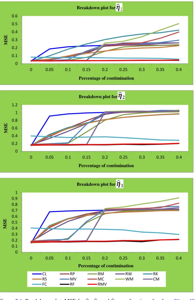
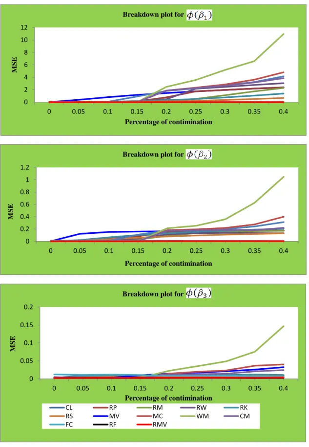
The breakdown plots and independent tests are employed as criteria of the robustness and performance of the estimators. Based on the computational studies and real data example, suggestions on the practical implications of the results are proposed.

(27)

15

2.1. Introduction

The CCA, originally proposed by Hotelling (1936), is a method that is used for gauging the linear relationship between two sets of variables. The aim of this method is to find basis vectors for two groups of variables achieve the correlations between the projections of the variables intothese basis vectors are mutually maximised.

The CCA has been widely applied in many statistical areas and a major advantage of the CCA is its application for dimension reduction (DR) and thus, it acts as a valuable tool that facilitates the understanding of complicated relationships among multidimensional variables (Das and Sen, 1998). The CCA is routinely discussed in many multivariate statistical analysis textbooks. For example, see Anderson (2003), Johnson and Wichern (2003) and Mardia et al. (1979).

Suppose that is a -dimensional random variable and is a -dimensional random variable, with . Furthermore, suppose that and have the covariance matrix (if it exists)

where and are non-singular. The objective of the CCA is to explore the linear relationship between and , as measured by the correlation between the linear combination (LC) of both groups of variables. Specifically, we look for

where is the Pearson correlation and the vectors and are called the first pair of canonical vectors. Let and , which are the first pair of canonical variates. According to Equation (2.2), the vectors and are not unique. The normalisation constraint is required in order to identify and uniquely (up to a sign).

(28)

16

While the and are useful, they do not capture the full dependence structure between and . To this end, higher order canonical vectors defined for as

are used where the pairs of canonical variates of order are and and

The correlation between the canonical variates of the th pair, , is the th canonical correlation. Moreover, the canonical vectors and are the eigenvectors corresponding to the eigenvalues of the matrices and or

and where

is the correlation matrix. The matrices in Equations and

have the same eigenvalues which correspond to the squared canonical correlations.

Hsu (1941) derived the limiting distributions (LD) of the canonical correlations in the case of a multivariate normal distribution. His result is valid under some very general assumptions regarding the population’s canonical correlations. The LD of the canonical vectors have been considered in several papers, see Anderson (1999) for an overview. Kettenring (1971) has generalised CCA to more than two sets of variables. Beaghen (1997) has used a canonical variate approach to analyse the means of repeated measurements. Anderson (1999) gave the complete LD of the canonical correlations and vectors assuming that the nonzero population correlations are distinct.

(29)

17

In order to estimate the canonical correlations and canonical vectors of the population, we first estimate by the sample covariance matrix followed by the computation of the eigenvalues and eigenvectors of the matrices and as given by Equation . This procedure works best when and are from a multivariate normal distribution; however, it appears to be less efficient with respect to outlying observations. From a practical point of view, it is well known that the sample covariance matrix is not resistant to outliers and thus the CCA based on this matrix will result in uncertain and misleading results. Similarly, Romanazzi (1992) showed that the classical canonical vectors and correlations are also sensitive to outliers. Consequently, in order to obtain accuracy and robustness, there is a need to estimate the population covariance matrix using robust approaches.

An apparent procedure to make CCA more robust, is to estimate a sample covariance or correlation matrix using methods that can account for outliers. One such approach was presented by Karnel (1991), who considered M-estimators as robust estimator of and then followed the classical approach. However, the robustness properties of the M-estimators are poor in high dimensions (Kent and Tyler, 1996). There are many estimators for robust multivariate location and dispersion (RMLD). The minimum covariance determinant (MCD) estimator is the fastest estimator of the RMLD that has been shown to be both consistent and having a high breakdown point. It has complexity, where (see Bernholt and Fischer, 2004). The complexity of the minimum volume ellipsoid (MVE) is far higher and there may be no known method for computing the projection based, constrained M, M-estimate of the scale of the residuals and the M-estimate of the parameters and Stahel–Donoho estimators (Olive and Hawkins, 2010).

(30)

18

Since the mentioned estimators are computationally time consuming, these estimators have been replaced by practical estimators which strike a balance between accuracy and computing cost. However, none of the workable estimators have been proved to be consistent and having a high breakdown point. For example, the fast minimum covariance determinant (FMCD) estimator, which is given in (Rousseeuw andVan Driessen, 1999), is used to replace the MCD estimator. The robust multivariate techniques (one of which is the robust canonical correlation) that claim to use the impractical MCD estimator actually use Rousseeuw and Van Driessen (1999) FMCD estimator.

Taskinen et al.(2006) obtained the influence function and asymptotic properties for CCA based on robust covariance matrix estimates. Following the approach suggested by Wold (1966), Filzmoser et al. (2000) devised a robust method for getting and

by using robust alternating regressions (RARs).

Branco et al. (2005) compared and discussed a number of approaches for robust canonical correlation analysis (RCCA). The authors proposed a robust method for obtaining all of the canonical variates using the RARs. Also, they stated that the CCA based on the FMCD estimator for the covariance matrix, is predominantly preferred due to itshigh breakdown point.

Zhou (2009) studied a weighted canonical correlation (WCC) method and its asymptotic properties. In the WCC, each observation is weighted based on its Mahalanobis distance. The author used the FMCD estimator to compute the Mahalanobis distance.

Jiao and Jian (2010) derived the asymptotic normal distributions of estimators of the projection pursuit method based on the CCA. Recently, Kudraszow and Maronna (2011) proposed a method for the RCCA based on the prediction approach.

(31)

19

Olive and Hawkins (2010) showed that the FMCD estimator is not a high breakdown estimator. The authors proposed practical consistent, outlier resistant estimators for multivariate location and dispersion. They suggested the FCH, RFCH and RMVN estimators. The authors suggested employing the RMVN estimator for CCA, discrimination, factor analysis, principal components and regression. The RMVN estimator uses a slightly modified method for reweighting such that it gives good estimates of for multivariate normal data, even when there are outliers in the data. Zhang and Olive (2009) used the RMVN estimator with principle component analysis. They suggested employing the RMVN estimator with the classical multivariate procedures. Zhang (2011) used the RMVN estimator for CCA.

Estimators with high complexity require considerable computing time and therefore, their usage will be seldom. The FCH, RFCH and RMVN estimators are roughly 100 times faster than the FMCD estimator (Olive, 2013).

Cannon and Hsieh (2008) suggested robust nonlinear canonical correlation analysis (NLCCA) to deal effectively with data sets with that have low signal-to-noise ratios. To achieve this, they employed a neural network model architecture of standard NLCCA. The authors substituted the cost functions, which were used to set the model parameters using more robust variants. The Pearson correlation was replaced by a biweight midcorrelation.

Wilcox (2004) studied the percentage bend correlation ( which is based on the M-estimators of location and the percentage bend measure of scale.

Wilcox (2005) stated that robust versions of the Pearson correlation are divided into two types. The first type consists of those that are robust against outliers, without taking into account the general structure of the data, whereas the second type takes into account the general structure of the data when dealing with outliers. In the literature,

(32)

20

the first and second types are referred to as the M correlation and O correlation, respectively. Moreover, Wilcox (2005) described the four types of M correlations as the , biweight midcorrelation ( ), winsorised correlation ( , and Kendall’s tau correlation ( ). Similarly, the author also presented a number of O correlation methods, such as the fast minimum volume ellipsoid (FMVE), FMCD and skipped measures of correlations. The FMVE and FMCD measures employ the central half of the data to estimate location, scatter, covariance and correlation. Skipped correlations are obtained by detecting the outliers using one of the multivariate outlier detection methods and then removing these outliers and applying some of the correlation coefficients to the remaining data (see Wilcox, 2005).

To the author’s knowledge, there is no study that has focused on replacing the Pearson correlation in the correlation matrix of the CCA with the and However, Olive and Hawkins (2010) recommended to employ the FCH, RFCH and RMVN estimators for the CCA, discrimination, factor analysis, principal components and regression and Zhang (2011) used the RMVN for CCA. Until now there has been no research employed regarding the FCH and RFCH estimators for estimating the covariance matrix in the CCA. To this end, the goal of this chapter is to get RCCA methods that depend on the and in the correlation matrix. Furthermore, we aim to employ the FCH and RFCH estimators in order to estimate the covariance matrix in the CCA to obtain RCCA and then compare these estimators with other known estimators.

In this chapter, we conduct a comparative study to explore the performance of 13 different estimators for canonical vectors and correlation. Simulation studies have been used in order to compare the numerical performances of the 13 different estimators

(33)

21

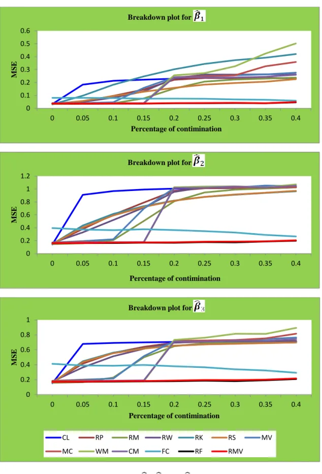
under different sampling schemes. To assess the robustness of the estimators, we use the breakdown plots and apply the test of independence.

In Section 2.2, different robustifications of CCA are discussed. In Section 2.3, the different estimators are compared using simulation studies. In Section 2.4, the breakdown plots in order to study the robustness of the estimators are used. In Section 2.5, tests of independence are done for the different estimators. An application is used to evaluate the methods in Section 2.6. The conclusions are summarised in Section 2.7.

2.2. RCCA based on robust correlation and robust covariance

matrices.

2.2.1. The percentage bend correlation (

)

Let a special case of Huber’s function be defined as

Furthermore, let and be the respective population medians for the random variables and and then define as the solution to the following equation:

where .

Let and denote the percentage bend measure of the location for and ,

respectively. Furthermore, let and , such that

.

(34)

22

The percentage bend correlation between and is:

where and is a robust measure of the linear association between and , such that the variables and are said to be independent when . The

depends, in part, on which is a generalisation of the median of the absolute deviations from the median (MAD).

The Huber’s function is selected to be used in the percentage bend correlation for a number of reasons. Firstly, Huber’s function is a monotonic function. Secondly, Huber’s function gives a consistent estimator of location. Thirdly, it has the convenient feature of a single iteration being sufficient in the application. Finally, when

, the resulting gauge of scale is a gauge of dispersion (Wilcox, 1994). This means, is a measure of dispersion when .

In order to estimate the percentage bend correlation,

1) Let , ),…., , , be a random sample. Let be the sample median for the observations . Select a value for , where .

2) Compute and and let , where

are the values written in ascending order.

3) Compute and , where is the number of values, such that and is the number of values, such that .

(35)

23

4) Set . Repeat these computations for the values, .

5) The estimated percentage bend correlation ( ) between and is:

where,

, , and .

In order to test the hypothesis when and are independent, we need to compute:

is rejected if , the quantile of distribution with degrees of freedom (D.F) (Wilcox, 2005).Here, is a significance level.

(36)

24

2.2.2. The biweight midcorrelation (

)

Let be any odd function and let and be any measure of location for random variables and , respectively. Let and be some measure of scale for random variables and , respectively. Let be some constant and let:

and . Then, a measure of covariance between and is:

where is the derivative of .

and the corresponding measure of correlation is given by

Wilcox (2005) chose as the biweight function and , where the biweight function is defined as follows:

Let and denote the respective medians calculated from the random sample

.

Define and then the and

(37)

25

Let

and

It follows that the sample biweight midcovariance between and is

and the bi-weight mid-correlation is then given by:

To test the null hypothesis when and are independent, we need to compute the test statistic

Under , we reject if , the quantile of t distribution with D.F .

2.2.3. The winsorised correlation (

)

Let and be two random variables. Then, the population winsorised correlation between and is:

where is the population winsorised standard deviation of and is the winsorised expected value of . We can obtain the winsorised standard deviation and the winsorised expected value by computing the usual standard deviation and expected value, based on the winsorised observations.

(38)

26

In order to estimate , based on the random sample ( , first winsorise the observations by computing the values as follows:

where is the number of observations trimmed, or winsorised, from each end of the distribution, corresponding to the group. Then is estimated by computing the Pearson’s correlation with the values:

To test the null hypothesis

we need to compute:

Under , we reject if , the quantile of t distribution with D.F , where is the effective sample size and equal to the number of pairs of observations that are not winsorised.

2.2.4. Kendall’s tau correlation (

)

Kendall’s tau correlation is a nonparametric M-type correlation. Because of being resistant to outlying observations, it is often said to be robust. Consider two pairs of observations and , such that and with the assumption that tied values never occur. If , then and will be concordant; otherwise

(39)

27

For pairs of points, let

Kendall’s tau correlation formula is

Although Kendall’s tau correlation provides resistance against outliers, the presence of outliers can substantially change its value if the percentage of outliers is greater than 0.05.

Under independence, the population Kendall’s tau correlation . To test the null hypothesis

we compute:

If , our decision will be rejecting .

For the sake of comparison the canonical correlation estimators based on Kendall’s tau correlation with other canonical correlation estimators, we apply the transformation

to obtain a consistent estimator under normality.

2.2.5. Spearman’s rho correlation (

)

Spearman’s rank correlation is the most popular non-parametric correlation, which is a Pearson correlation based on the ranks of the observations. This correlation provides resistance against outliers; however, outliers that are properly placedcan alter

(40)

28

its value considerably. In applications, a simple procedure can be used to calculate . In order to estimate based on a random sample the formula is given by:

where , which is the difference between the ranks of each observation on the two variables (Myers and Arnold, 2003).

If the sampling from a bivariate normal distribution, does not estimate the same quantity as the Pearson correlation. To compare the estimators of canonical correlations based on spearman’s rho correlation with other estimators, we need to apply the transformation in order to obtain a consistent estimator under normality.

Under the statistical independence, . To test the following hypothesis

We need to calculate the statistic:

should be rejected if , the quantile of t distribution with D.F

(41)

29

2.2.6. The MVE estimator

The MVE estimator is an affine equivariant estimator that has a high breakdown point (see Rousseuw and Leroy, 1987). Assume any ellipsoid containing 50% of the data. The idea is to find the ellipsoid having the smallest volume among all the ellipsoids. When this ellipsoid is found, the mean and covariance matrix of its points are taken as the estimated measures of location and scatter, respectively. In the multivariate normal model, the covariance matrix needs to be rescaled for consistency. In general, the group of all of the ellipsoids containing half of the data is very large, therefore the approximation must be used to find the MVE.

Let , rounded down to the nearest integer. The approach for computing the FMVE estimator is summarised as follows:

1. Select random points from the available points without replacement.

2. Compute the volume of the ellipse containing these points.

3. Repeat step 1 and 2 many times.

The FMVE ellipsoid is the set of points giving the smallest volume (Wilcox, 2005).

2.2.7. The MCD estimator

The MCD estimator is also an affine equivariant estimator that has a high breakdown point. The difference between the MCD and MVE estimators is that rather than searching for the subset of 50% of the data that has the smallest volume, the MCD estimator searches for the 50% of the data that has the smallest generalised variance.

(42)

30

The MCD estimator searches for 50% of the data that is most tightly clustered together among all of the subsets containing 50% of the data, as measured by the generalised variance. Like the MVE estimator, the group of all subsets of 50% of the data is very large, hence an approximate method must be used. Rousseeuw and Van Driessen (1999) described an FMCD algorithm employed to achieve this aim. After we find an approximation of the subset of 50% of the data that minimise the generalised variance, we can obtain the MCD estimate of location and scatter by computing the usual mean and covariance matrix, based on its points. The MCD estimator has several merits over the MVE. The MCD estimator is more efficient than the MVE estimator because the MCD is asymptotically normal, whereas the MVE has a lower rate of convergence ( Rousseeuw and Van Driessen, 1999). In our comparative study, we used the FMCD and reweighted MCD (WMCD) measures as practical approximations for the MCD.

2.2.8. The constrained M-estimators

Rocke (1996) suggested a modified biweight estimator, which is a constrained M-estimator, where values of and are to be determined and the non-decreasing function ξ is defined as:

ξ

(43)

31

The values of and can be selected to obtain the wanted breakdown point and the asymptotic rejection probability (ARP). The ARP is the probability that an observation will obtain weight equals to zero when the size of the sample is huge. If the ARP is , then and are determined by ξ and

where is a constant and is the quantile of a chi-squared distribution with D.F. Rocke (1996) showed that this estimator can be computed iteratively.

2.2.9. The FCH estimator

Olive and Hawkins (2010) proposed the FCH estimator. The FCH estimator uses the consistent DGK estimator in (Devlin et al., 1981) and the high breakdown median ball (MB) estimator in (Olive, 2004) as attractors. An attractor is one of the trial fits used by the robust estimator. Therefore if the robust estimator draws elemental sets and then refines them with concentration, then the refined elemental sets are the attractors. The FCH estimator also uses a location criterion to choose the attractors. If DGK location estimator has a greaterEuclidean distance from than 50% of the data, where is the coordinate-wise median, then FCH uses the MB attractor. The FCH estimator uses only the attractor with the smallest determinant if

where is the Euclidean distance from and is identity matrix. Here refers to the Euclidean distance.

(44)

32

Let be the attractor that is used, where and are the location and dispersion estimators, respectively. Then, the estimator takes and

where is the th squared sample Mahalanobis distance, which takes the form

_{for each observation, the}

is the

percentile of a chi-squared distribution and is the FCH estimator. Olive and Hawkins (2010) showed that the FCH estimator is a high breakdown estimator and is non-singular, even with up to nearly 50% outliers.

2.2.10. The RFCH estimator

Olive and Hawkins (2010) used two standard reweighting steps to produce the RFCH estimator. Let be the traditional estimator computed to cases with

and let

Then, let be the traditional estimator computed to the cases with

and let

(45)

33

2.2.11. The RMVN estimator

Olive and Hawkins (2010) suggested the RMVN estimator as a RMLD estimator and they showed this estimator is a consistent estimator of where . TheRMVN estimator uses a slight modification to a standard reweighting method, such that the RMVN estimator produces good estimates of for multivariate normal data, even if outliers are present (Olive and Hawkins, 2010).

The RMVN estimator uses with based on cases. Let and

Then, let

be the traditional estimator computed to cases with

.

,

where .

Olive (2013) shows that the FCH, RFCH and RMVN methods of RCCA produce consistent estimators of the th canonical correlation on a wide category of elliptically contoured distributions, see (Olive, 2013).

(46)

34

2.3. Simulation study

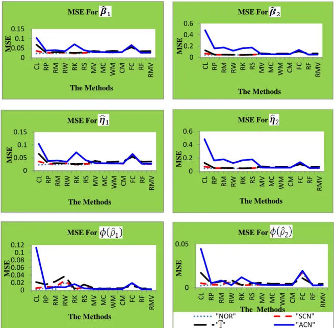
In this section, we employ a simulation study to compare the different methods. We considered the following:

CL is the classical CCA based on eigenvalues and eigenvectors of the matrices (2.5), which were estimated using the sample covariance matrix.

RP, RM, RW, RK and RS are the CCA based on eigenvalues and eigenvectors of the matrices (2.6) after we used , , , and , respectively, instead of the Pearson correlation.

MV, MC, WM, CM, FC, RF and RMV are the CCA based on eigenvalues and eigenvectors of the matrices (2.5), which are estimated using the FMVE, FMCD, WMCD, CM, FCH, RFCH and RMVN estimators, respectively, instead of the classical sample covariance matrix.

The functions pball and winall from the Wilcox package at (http://www.unt.edu/ rss/class/mike/Rallfun-v9_2.txt) have been used to compute the correlation matrices of and , respectively. The function bicor from the package (weighted gene co-expression network analysis) (WGCNA) has been used in order to compute the midcorrelation matrix. The base functions cor(,method = c("kendall")) and cor(, method = c("spearman")) have been used to calculate Kendall and Spearman correlation matrices, respectively.

The base functions cov.mve and cov.mcd have been used for computing the FMVE and FMCD covariance matrices. The functions covRob (,estim="weighted") and

covRob (,estim="M") from the package (robust) have been used to calculate the weighted MCD (WM) and constrained M (CM) covariance matrices, respectively. The function covfch from the package (rpack.txt) at (www.math.siu.edu/olive/rpack.txt) has

(47)

35

been used for calculating the FCH and RFCH covariance matrices and the function

covrmvn has been used to calculate the RMVN covariance matrix.

We follow the simulation settings given in Branco et al. (2005). samples with size have been generated. We have assumed and . The choices for are summarised in Table 2.1.

Following the work of Branco et al. (2005), the following sampling distributions were assumed:

1) Normal distribution (NOR), .

2) Multivariate distribution with three D.F ( ).

3) Symmetric contamination (SCN), where of the observations have been generated from and have been generated from .

4) Asymmetric contamination (ACN), where of the observations have been generated from and of the observations equals the point (where is the trace of ).

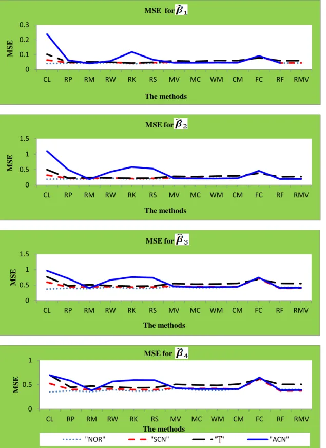
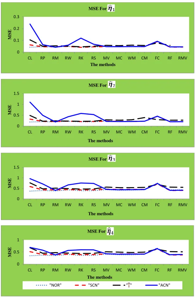
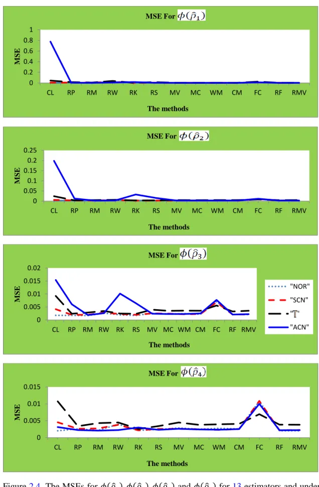
The estimated parameters for a replication ( are denoted by , , and for . We compare the estimated parameters with the “true” parameters , , and . The true parameters were computed from the specific matrix . The mean squared error (MSE) has the following forms:

(48)

36 ,

Table 2.1. Simulation Setup. and . 2 2 4 4

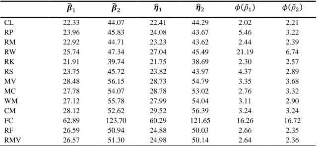
Table 2.2. The of , , , , and multiplied by for 13 different methods, when the data is from NOR, and .

CL 22.33 44.07 22.41 44.29 2.02 2.21 RP 23.96 45.83 24.08 43.67 5.46 3.22 RM 22.92 44.71 23.23 43.62 2.44 2.39 RW 25.74 47.34 27.04 45.49 21.19 6.74 RK 21.91 39.74 21.75 38.69 2.30 2.57 RS 23.75 45.72 23.82 43.97 4.37 2.89 MV 28.48 56.15 28.73 54.79 3.35 3.68 MC 27.78 54.07 28.78 53.02 2.76 3.32 WM 27.12 55.78 27.99 54.04 3.11 2.90 CM 28.12 52.62 29.52 56.39 3.24 3.24 FC 62.89 123.70 60.29 121.65 16.26 16.72 RF 26.59 50.94 24.88 50.03 2.66 2.35 RMV 26.57 51.30 24.98 50.14 2.64 2.36

(49)

37

Table 2.3. The of , , , , and multiplied by for 13 different methods, when the data is from SCN, and .

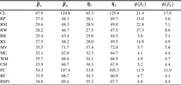
Table 2.4. The of , , , , and multiplied by for 13 different methods, when the data is from , and .

(50)

38

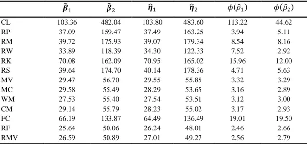
Table 2.5. The of , , , , and multiplied by for 13 different methods, when the data is from ACN, and .

Table 2.6. The of , , , , , , , and multiplied by for 13 different methods, when the data is from NOR, and . CL 40.2 189.3 370.0 350.8 42.1 189.5 367.5 345.0 2.0 2.3 1.7 2.0 RP 43.0 203.0 396.6 372.7 45.0 203.6 395.7 369.3 5.1 2.6 1.7 2.6 RM 41.0 194.5 379.4 357.4 43.4 195.6 377.5 353.0 2.4 2.2 1.7 2.1 RW 46.0 223.1 431.2 398.8 48.9 220.1 429.8 397.6 20.7 5.6 2.6 4.0 RK 38.3 196.4 391.9 366.7 40.4 197.4 388.9 362.1 2.4 2.5 1.9 2.2 RS 42.0 201.2 393.1 368.9 44.8 201.5 391.3 364.6 4.3 2.5 1.7 2.4 MV 47.7 223.0 445.7 419.9 47.9 224.8 439.9 411.0 2.9 3.4 2.6 2.9 MC 45.7 212.7 412.2 388.6 47.7 213.2 412.5 387.8 2.7 2.9 2.3 2.5 WM 45.8 219.4 414.0 376.5 45.5 219.9 418.7 383.5 2.9 2.8 2.4 2.7 CM 47.2 222.1 434.5 411.4 45.8 222.2 434.9 406.5 2.3 2.6 2.2 2.6 FC 86.0 440.4 744.2 651.4 90.4 446.3 746.0 660.0 13.0 9.9 7.0 10.8 RF 43.6 205.9 427.1 402.4 43.4 207.6 426.6 401.7 2.5 2.5 2.1 2.0 RMV 43.9 206.8 426.4 401.4 43.5 208.6 426.9 402.0 2.6 2.5 2.1 2.0

Some statistical methods for dimension reduction