Two-Stage Stochastic Mixed Integer Linear Optimization

(1)

Lehigh Preserve

Theses and Dissertations

2015

Two-Stage Stochastic Mixed Integer Linear

Optimization

Anahita Hassanzadeh

Lehigh University

Follow this and additional works at:

http://preserve.lehigh.edu/etd

Part of the

Industrial Engineering Commons

This Dissertation is brought to you for free and open access by Lehigh Preserve. It has been accepted for inclusion in Theses and Dissertations by an authorized administrator of Lehigh Preserve. For more information, please [email protected].

Recommended Citation

Hassanzadeh, Anahita, "Two-Stage Stochastic Mixed Integer Linear Optimization" (2015).Theses and Dissertations. 2629.

(2)

Two-Stage Stochastic Mixed

Integer Linear Optimization

by

Anahita Hassanzadeh

Presented to the Graduate and Research Committee of Lehigh University

in Candidacy for the Degree of Doctor of Philosophy

in

Industrial Engineering

Lehigh University

(3)

(4)

the requirements for the degree of Doctor of Philosophy.

Date

Dr. Theodore K. Ralphs Dissertation Advisor

Committee Members:

Dr. Theodore K. Ralphs, Committee Chair

Dr. Shabbir Ahmed

Dr. Simge K¨u¸c¨ukyavuz

Dr. Aur´elie C. Thiele

(5)

Acknowledgements

First and foremost, I would like to thank my advisor, professor Ted Ralphs, whose ideas, inspirations, guidelines, and constant support made this work possible. I have the deepest appreciation for his enthusiasm and patience and especially for his perspectives on ways to approach challenging problems. I am very grateful for the countless hours he has spent mentoring me in my research and my career.

I would also like to thank my thesis committee members, professors Aurélie Thiele and Luis Zuluaga from the Department of Industrial and Systems Engineering at Lehigh University, as well as my external committee members professors Shabbir Ahmed and Simge Kü¸cükyavuz, for their help and suggestions for enhancing this thesis.

My special thanks go to two very supportive faculty members of the Department of Industrial and Systems Engineering at Lehigh University, professor Katya Scheinberg and professor Frank Curtis. Dr. Scheinberg has been a true role model for me, to whom I owe the very valuable experience I gained during my internship in the second year of my studies. I appreciate the time and effort she has put in helping me with my career during my time at Lehigh and afterwards. My thanks also go to a great teacher, Dr. Curtis, whose office door has always been open to me and who has generously answered my questions many times. I would also like to thank professor Asgeir Tomasgard who provided me with the opportunity to visit the stochastic optimization research team at the Norwegian University of Science and Technology.

My years at Lehigh could never be as fulfilling without my amazing friends. Thank you Inkeri and Doug Coleman, Kiana Kouchakzadeh, Leyla Mohseninejad, Joyita Bhadra,

(6)

I also owe my profound gratitude to my family. I would like to thank my husband, Neil Dexter, for his continuous encouragement and support in the past four years. My heartfelt thanks also go to my parents, my brother, Babak, and my sister, Ainaz, to whom I owe every success of my life. Finally, my thanks go to the Gonglewskis for their love and support.

(7)

List of Tables

3.1 Assumptions made in related algorithms . . . 100

4.1 Iterations of the Generalized Benders’ algorithm applied to Example 4.6 . 139

4.2 Iterations of the Generalized Benders’ algorithm applied to Example 4.2 . 139

4.3 Size of the deterministic equivalent of the test instances in Example 4.2 . 140

4.4 Performance of the algorithm applied to problems in Example 4.2. . . 140

4.5 The deterministic equivalent of SSLP instances . . . 143

4.6 Generalized Benders’ algorithm applied to SSLP instances . . . 148

4.7 Generalized Benders’ algorithm with warm start applied to SSLP instances149

4.8 The deterministic equivalent of the SIZES instances . . . 153

4.9 Generalized Benders’ algorithm applied to SIZES instances . . . 153

(10)

List of Figures

1.1 The LP value function (1.12) . . . 12

1.2 The LP value function (1.12) and the set of its subgradients at zero. . . . 16

1.3 The MILP value function (1.20). . . 18

1.4 The objective function Ψ and second-stage value functionz in Example 1.4. 23 1.5 The value functions of two pure integer variations of (1.35) . . . 24

1.6 The objective and second-stage value functions for Example 1.6. . . 25

1.7 The constraints of (DE) . . . 26

2.1 The value functions (1.20) and (2.2). . . 34

2.2 The upper d-directional derivative of (1.20). . . 36

2.3 MILP Value Function of (2.15). . . 42

2.4 The value function of the continuous restriction of (2.16) and a translation. 44 2.5 Value Function (2.19). . . 47

2.6 The MILP value function and the epigraph of the (CR) value function at the origin. . . 51

2.7 MILP value function (2.22) with no local minimum. . . 52

2.8 Linear and convex MILP and CR value functions to (2.23). . . 53

2.9 The value function of the MILP in (2.22) . . . 56

2.10 MILP Value Function of (2.26) with BI = [0,2].. . . 58

2.11 Local stability sets and corresponding integer part of solution in (2.15). . 67

2.12 The scaled PILP value function (2.32). . . 70

(11)

2.15 Normalized approximation gap vs. iteration number. . . 80

3.1 Strong dual functions from warm-starting branch-and-bound - RHS = 5.5 107 3.2 Strong dual functions from warm-starting branch-and-bound - RHS = 11.5 108 3.3 Strong dual functions from warm-starting branch-and-bound - RHS = 4 . 109 3.4 Strong dual functions from warm-starting branch-and-bound - RHS = 10 110 3.5 Branch-and-bound tree and value function correspondence for Example 1.6 114 3.6 The MILP value function corresponding to the tree in Figure 3.5 . . . 115

3.7 Strengthened dual functions from warm-starting (a) . . . 118

3.8 Strengthened dual functions from warm-starting (b) . . . 119

4.1 Use of SYMPHONY warm-start with parameter modification . . . 131

4.2 Use of SYMPHONY warm-start with problem data modification . . . 133

4.3 Sketch of the main module. . . 134

4.4 Warm-starting the solution to each scenario . . . 136

(12)

Abstract

The primary focus of this dissertation is on optimization problems that involve uncer-tainty unfolding over time. In many real-world decisions, the decision-maker has to make a decision in the face of uncertainty. After the outcome of the uncertainty is observed, she can correct her initial decision by taking some corrective actions at a latertime stage. These problems are known asstochastic optimization problems with recourse. In the case that the number of time stages is limited to two, these problems are referred to as two-stage stochastic optimization problems. This class of optimization problems is the focus of this dissertation. The optimization problem that is solved before the realization of uncertainty is called thefirst-stage problem and the problem solved to make a corrective action on the initial decision is called the second-stage problem. The decisions made in the second-stage are affected by both the first-stage decisions and the realization of random variables. Consequently, the two-stage problem can be viewed as a parametric optimization problem that involves the so-calledvalue function of the second-stage prob-lem. The value function describes the change in optimal objective value as the right-hand side is varied and understanding it is crucial to developing solution methods for two-stage optimization problems.

In the first part of this dissertation, we study the value function of a MILP. We review the structural properties of the value function. We propose a discrete representation of the MILP value function. We show that the structure of the MILP value function arises from two other optimization problems that are constructed from its discrete and continuous components. We show that our representation can explain certain structural properties

(13)

then provide a simplification of theJeroslow Formula obtained by applying our results. Finally, we describe a cutting plane algorithm for its construction and determine the conditions under which the proposed algorithm is finite.

Traditionally, the solution methods developed for two-stage optimization problems consider the problem in which the second-stage problem involves only continuous vari-ables. In recent years, however, two-stage problems with integer variables in the second-stage have been visited in several studies. These problems are important in practice and arise in several applications in supply chain, finance, forestry and disaster management, among others. The second part of this dissertation concerns the development and imple-mentation of a solution method for the two-stage optimization problem where both the first and second stage involve mixed integer variables. We describe a generalization of the classical Benders’ method for solving mixed integer two-stage stochastic linear optimiza-tion problems. We employ the strong dual funcoptimiza-tions encoded in the branch-and-bound trees resulting from solution of the second-stage problem. We show that these can be used effectively within a Benders’ framework and describe a method for obtaining all required dual functions from a single, continuously refined branch-and-bound tree that is used to warm start the solution procedure for each subproblem.

Finally, we provide details on the implementation of our proposed algorithm. The implementation allows for construction of several approximations of the value function of the second-stage problem. We use different warm-starting strategies within our proposed algorithm to solve the second-stage problems, including solving all second-stage problems with a single tree. We provide computational results on applying these strategies to the stochastic server problems (SSLP) from the stochastic integer programming test problem library (SIPLIB).

(14)

Introduction

We begin by considering the general optimization problem

inf

x∈Uf(x), (1.1)

where the f :Rn→R is called the objective function and the setU ⊆Rn is the feasible

regionof the problem. A vectorx∈U is referred to as afeasible solution, which expresses adecision, andf(x) is its associatedsolution value, or the cost of the decision. If the set

U is an empty set, the problem is called infeasible. Any x∗ ∈U such thatf(x∗) =zG is called anoptimal solution andf(x∗) is called the optimal value.

The optimization problem (1.1) assumes a single decision-maker with a single objective function making a single set of decisions at a single point of time where the descriptions of the objective functionf and the feasible region U are fixed and known. Optimization problems in real-world, however, often involve multiple decision-makers with congruent or conflicting objective functions that make decisions in multiple points of time. The decisions made at a given point of time often affect future decisions and are affected by future uncertainty themselves. Several frameworks have been developed that extend (1.1) by adding one or more of these features to it. One such framework ismulti-objective optimization, which extends the traditional framework to capture the decisions involving a single decision-maker trading off multiple objective functions. The setting of

(15)

multi-objective optimization problems is still restricted to centralized decision processes that are controlled by a single decision-maker. A class of optimization problems that general-izes this setting ismulti-leveloptimization problems. This setting allows for the modeling of situations that involves several levels of decision-maker whose decisions are made se-quentially with each decision potentially affecting the decisions made in higher or lower levels of the overall hierarchy. Multi-level optimization problems provide a representa-tion of game-theoretic processes in which decision-makers make sequential decisions in multiple rounds. In this setting each player strives to optimize her individual, competing objective function by making a decision that takes into account the reactions of the other players. This setting assumes perfect information, meaning that the decision-maker is able to predict the reaction of other players to her decision.

Both multi-objective and multi-level optimization problems assume that at the time of decision-making, the decision-makers have complete information about the parameters of the optimization problems to be solved by other players lower in the hierarchy. In this sense, these problems are deterministic. In practice, however, one frequently faces problems where the actual cost or feasibility of a decision is only determined after the decision is made. There are several frameworks that allow for modeling uncertainty in optimization problems. Like the deterministic case, these frameworks allow for single or multiple decision makers who make decisions hierarchically or at a single point of time. We discuss these frameworks more formally next.

1.1 Optimization Under Uncertainty

We now consider a generalization of (1.1) formulated as

inffω(x)

s.t. gi(x, ω)≤0, i= 1, . . . , m, ω∈Ω,

(1.2)

whereωrepresents an uncertain element of the problem that comes from a set of outcomes, Ω. The uncertain element is said to berealized orobserved when it actually happens and

(16)

its value is observed.

Chance-Constrained Optimization Problems. In problem (1.1), a feasible point must satisfy all the constraints, gi(x, ω) ≤ 0 for i = 1, . . . , m and ω ∈ Ω.

Chance-constrained optimization, on the other hand, allows for incorporating uncertainty by relaxing some or all of the constraints probabilistically. The goal in solving a chance-constrained optimization problem is to satisfy the constraints in “most” cases. Chance-constrained models assume that the uncertain terms in the problem can be modeled as random variables derived from a probability distribution that is known or can be estimated. That is, Ω is assumed to be the set of all possible outcomes of a probability space. The requirement in the constraints is to ensure that for a given decision ˆx, the probability that the constraint is violated is no more than a given value αi where 0 ≤

αi ≤1,i= 1, . . . , m.

Let prob{gi(x, ω)≤0}denote the probability that the ith constraint holds. Then the chance-constrained problem can be written as

minf(x)

s.t.prob{gi(x, ω)≤0} ≥1−αi fori= 1, . . . , m.

(1.3)

In the above case, the constraints are assumed to be independent of each other. Chance-constrained problems can also model the case where interactions exists between the con-straints. In this case, the set of constraints can be written as

prob{gi(x, ω)≤0 for i= 1, . . . , m} ≥1−α.

Chance-constraints are appealing from a modeling perspective, as they provide means to model real-world requirements of an optimization problem such as the desired service-level. However, determining the probability levels and information about the joint proba-bility distribution with potentially a large number of random variables can be a challenge.

(17)

Robust Optimization Problems. Another framework that is used to model uncer-tainty is robust optimization. This framework captures the case where a single decision-maker aims to protect against the risk by a one-time decision that is made in the presence of uncertainty. In particular, the decision-maker is interested in minimizing the maxi-mum cost that can incur as a result of the uncertainty. Here, the minmax goal is used to protect the decision against the worst-case outcome. The robust framework assumes the uncertainty belongs to an uncertainty set. That is, the set of outcomes where the uncertain element is coming from is this uncertainty set. This set can be a complicated convex or polyhedral set, or simply is the bounds of the uncertain parameters. This allows for modeling uncertainty whose specific probability distribution is not known. This is an appealing property where historical data is not available and probabilities are challenging to estimate.

The general model of a robust optimization problem is

min max γ0∈γ0

f(x, γ0)

s.t. g(x, γ)≤0, γ ∈Γ,

(1.4)

whereγ denotes the uncertain elements and Γ0 and Γ are given uncertainty sets and have

special forms such that the problem can be solved with efficient algorithms. For example, these sets can be assumed to be convex or polyhedral.

Stochastic Optimization Problems. A critical difference between models of opti-mization problems that involve uncertainty origins from the way they immunize the deci-sion against the outcome of uncertain elements. While in the robust optimization frame-work the goal is to minimize the maximum possible cost, in the stochastic optimization problem the expected cost of decisions is minimized. In this scheme, the random cost is replaced by itsexpected value, denoted byE. In this case, the general problem (1.2) takes the form

(18)

When the probability space Ω is discrete and finite, ω represents which one of a finite number of explicitly enumerated scenarios is realized and pω represents the probability of such an outcome. Then, (1.5) can be written as

inf X ω∈Ω

pωf(x, ω). (1.6)

Similarly, if Ω represents a continuous space with the probability density function ρ(ω) defined forω ∈Ω, then (1.5) is equivalent to

inf

Z

Ω

f(x, ω)ρ(ω)dω. (1.7)

There are studies that consider random variables that follow an infinite distribution. For a review of the assumptions and properties of this case we refer the reader to (Ruszczynski and Shapiro, 2003). A standard approach to solve stochastic optimization problems is by generating scenarios. A scenario is a realization of a future event consisting of an outcome of random variables. In the case of stochastic optimization, scenarios can be constructed by drawing samples from the known probability space(s) and observing their values, rendering the outcome space where the uncertainties come from finite.

Both the chance-constrained and robust optimization frameworks consider decisions that are made at a single point of time. In practice, however, the decision-maker is of-ten able to react to the new situation as new information becomes available. While the decision-maker makes the initial decision in the face of the unknown, she can takerecourse

actions at one or more points of time in future. This framework is known as stochastic optimization with recourse. This framework resembles multi-level optimization problems in that decisions are made dynamically and they change according to the realization of uncertainty. We can also view these problems as multi-level problems in which decision makers cooperate and their objectives align with one another and therefore, can be in-terpreted as a problem with a single decision-maker. Stochastic optimization problems, however, extend the multi-level framework by allowing uncertainty to be explicitly

(19)

mod-eled. Like chance-constrained optimization, stochastic optimization assumes a known probability distribution where the random variables can be drawn from a probability space.

A classical example of stochastic optimization problems with recourse is the unit com-mitment problem in which the utility company has to decide ahead of time whether to start up/shut down power generators to meet an unknown future demand load. In this case, the distribution of demand maybe known or can be estimated from statistical data. Other examples arise in areas such as disaster planning, where decisions on dispatching storm/wildfire protections equipment are made before the weather conditions are ob-served. In supply chain management, for example, decisions on the quantity of order for retail goods are made with non-deterministic demand and holding costs.

Studying stochastic optimization problems with recourse is the focus of this thesis. We mentioned earlier that in the setting of stochastic optimization, the decision-maker has to commit to certain actions before the unknown terms are observed (the problems is, of course, deterministic if she can postpone making commitments after the observation). Stochastic optimization with recourse also assumes there is a possibility of recourse that allows the decision-maker to correct her earlier decisions in one or multiple times in future. This decision-making process can be illustrated with:

x0 ∈U0 initial decision ω1 ∈Ω1 observation x1∈U1(x0) recourse decision ω2 ∈Ω2 observation .. . ωN ∈ΩN observation xN ∈UN(x0, . . . , xN−1) recourse decision.

(20)

illustration, the initial stagex0 is followed byN recourse actions taken inN future time

stages. The numberNis usually assumed to be finite. Typically, a stochastic optimization problem that involves a large number of time stages is very challenging to solve. A simpler variation that is often considered is where the first observation is followed by only one corrective decision. The resulting recourse problems are important in theory and practice and are referred to astwo-stage stochastic optimization problems. Next, we introduce two fundamental concepts in this class of problems.

In this thesis, we focus on two-stage stochastic optimization problems which involves random variables that follow a discrete distribution. We consider the case where all or some of the variables in the first or second-stage problems have to be integer. We also focus on the case where the objective function and constraints in both stages are linear functions. These problems lie at the intersection of stochastic linear optimization with recourse and discrete linear optimization. We review these problems in more depth in the upcoming Section 1.3. In the remainder of this section, we provide an overview of some of the fundamental concepts in discrete optimization that are necessary for this work. We then review the principle of Benders’ decomposition applied to optimization problems and in particular, to two-stage linear optimization problems.

1.2 Discrete Optimization

A mixed integer linear optimization problem (MILP) is a variation of the optimization problem (1.1) with a linear objective function and a polyhedral feasible region where a subset of the variables areinteger variables. Consider the nominal MILP instance

inf x∈Sc

>_x, _(MILP)

wherec∈Rn is the objective function vector and S ={x∈Zr+×Rn −r

+ |Ax= ˜b} is the

feasible region, described by A ∈ Qm×n, b ∈ Rm, and a scalar r indicating the number of integer variables. We refer to this problem as the primal problem. Throughout the thesis, we assume rank(A, d) =rank(A) =m. The variables of the instance are indexed

(21)

on the set N = {1, . . . , n}, with I = {1, . . . , r} denoting the index set for the integer variables andC={r+ 1, . . . , n} denoting the index set for the continuous variables. For any D⊆N and a vector v indexed on N, we denote by vD the sub-vector consisting of the corresponding components of v. Similarly, for a matrix M, we denote by MD the sub-matrix constructed by columns of M that correspond to indices inD.

In many applications of integer optimization, we are interested in a parametric version of (MILP) that allows for analyzing the changes in the optimal value of the problem when the parameters of the problem are perturbed. In the case of two-stage stochastic optimization problems, it will be clear soon that we are interested in the change in the optimal value as the right-hand side of a given MILP instance is modified. In what comes next, we introduce a function that is designed to provide such information.

Value Function

The value function of a MILP is a function z : Rm → R∪ {±∞} that describes the change in the optimal solution value of a MILP as the right-hand side is varied. In the case of (MILP), we have

z(b) = inf x∈S(b)c >_x _∀_b_∈_B, _(1.8) where for b∈_Rm_,_S₍_b_{) =}_{_x_∈ Zr+×Rn −r

+ |Ax=b}. The set of right-hand sides, B, is

the set of real vectors such that the corresponding feasible region is non-empty. That is,

B ={b∈ Rm |S(b)6= ∅}. By convention, we let z(b) =∞ if S(b) =∅ and z(b) = −∞ when the infimum is not attained at any feasible point. To simplify the presentation, we assume thatz(0) = 0.

A special case of a MILP is where none of the variables have integrality restrictions, e.g.,r= 0. The resulting problem is known as a linear optimization problem (LP) and is defined as

inf x∈SLP

(22)

where the feasible regionSLP is defined as

SLP ={x∈Rn+|Ax= ˜b}. (1.10)

We will discuss in Chapter2that the structure of the MILP value function (1.8) is closely related to that of a certain LP. We define the LP value function as

zLP(b) = inf x∈SLP(b)

c>x ∀b∈B, (1.11)

where forb∈_Rm_,_S

LP(b) ={x∈Rn+|Ax=b}. Let us look at an example first.

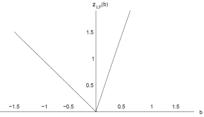
Example 1.1. Consider

zLP(b) = inf 4x1+ 6x2+ 7x3

s.t. x1+ 2x2−7x3 =b x1, x2, x3 ∈R+.

(1.12)

The function zis plotted in Figure 1.1. We have

zLP(b) =        −b ifb <0 3b ifb≥0,

From the figure we can see that the value function is a piecewise convex and continuous function. This structure arises from the properties of the so-calleddual functions to the LP value function. A dual function is simply a function that bounds the value function from below.

Definition 1.1. A functionf :Rm2 _→_R_{∪ {±∞}}_{is said to be}_dual _{to the value function}

z if

f(b)≤z(b) ∀b∈_Rm2_. (1.13)

(23)

Figure 1.1: The LP value function (1.12)

The properties of dual functions, as well as methods for constructing them are studied in the theory of duality. The goal is to construct dual functions that approximate the value function closely. In this respect, the value function is the best dual function. However, an explicit construction of the value function, as we will see later, can be very challenging. In practice, we often need a method to generate a dual function that provides the best bound for a given instance. This is done by solving an optimization problem for a given ˆ_b_{, called the}_{dual problem}

sup{f(ˆb)|f(b)≤z(b) ∀b∈Rm, f :Rm2 →R∪ {±∞}}. (1.14)

We call a dual function optimal if it is optimal for the problem (1.14). Although the definition of a dual problem allows for a wide range of dual functions to be selected, the search space in (1.14) is often in practice restricted to special families of functions which can be constructed with tractable methods.

Consider the case of an LP. Let us restrict the dual functions to be linear. For a given ˆ_b_∈_Rm_{, the dual problem (}_1.14_{) can be written as}

(24)

wherezLP is defined in (1.11). The problem (1.16) is equivalent to

sup ν∈DLP

ˆ

b>ν, (1.16)

whereDLP ={ν ∈Rm |A>ν≤c}. The latter problem is another LP which is referred to as the dual to (1.9). The primal-dual relationship between the problems (1.9) and (1.16) is important to study the properties of the LP value function and construction of dual functions to it. The following result is key to LP duality.

Theorem 1.1. (LP weak and strong duality byBazaraa et al.(1990)) For a givenˆb∈_Rm

with finite zLP(ˆb), we have b>ν ≤ zLP(ˆb) for any ν ∈ Rm that is a feasible solution

to (1.16). Furthermore, there always exists an optimal solution ν∗ to the dual problem such thatf(b) =b>ν∗, b∈Rm is a strong dual function to the value function w.r.t. ˆb.

The first and second parts of the Theorem 1.1 are respectively known as the weak and strong duality theorems. As a consequence of the weak duality theorem, we have a dual function for the LP value function f(b) =b>ν, where ν is a feasible solution to the dual problem (1.16). This in fact holds even when the instance of the LP problem is not finite. The only case that the weak duality theorem does not hold is when both the dual and the primal problems are infeasible.

Strong and weak duality theorems reveal important structural properties of the LP value function. To explain this relation, we first need some definitions.

Definition 1.2. A set C ⊆_Rn _{is a called a} _cone _{if for any} _x _∈ _C _and _λ_≥ _{0 we have}

λx∈C.

Furthermore, a polyhedron that can be described in the form S={x∈_Rn_:_Ax_≥₀_} for someA∈_Rm×n _{is called a}_{polyhedral cone}_.

Definition 1.3. The epigraph of the function f :Rn→R is defined as

epif ={(x, t)∈Rn×R:t≥f(x)}.

(25)

Let us defineKLP to be the polyhedral cone that is the positive linear span ofA, i.e.,

K_LP = {λ1A1. . .+λnAn : λ1, . . . , λn−r ≥ 0}, where Aj is the jth column of A. This cone is the set of right-hand sides over whichzLP is finite and plays an important role in the structure of the LP value function. We assume the coneK_LP is non-empty, therefore

D_LP 6=∅. Then, we can write the LP value function as

zLP(b) = sup ν∈DLP

ˆ

b>ν. (1.17)

Since D_LP 6= 0, from the Minkowski-Weyl theorem, we have that there exists a non-empty set{νi}i∈K, the set of a finite number of extreme points ofDLP indexed by setK. Furthermore, when DLP is unbounded, there exists a non-empty set of a finite number of extreme directions{dj}j∈L be indexed by set L. If the LP with right-hand side ˆb has a finite optimum, then

zLP(ˆb) = sup ν∈DLP ˆ_b> ν = sup i∈K ˆ_b> νi. (1.18)

Otherwise, for somej∈L, we have ˆb>dj >0 andzLP(ˆb) = +∞.

The convexity ofzLP follows from the representation (1.18), sincezLP is the maximum of a finite number of affine functions and is hence a convex polyhedral function (Bazaraa et al.,1990;Blair and Jeroslow,1977). For such a function, we can derive dual functions using its subgradient information. We discuss this next. The first following result guar-antees the existence of subgradients for zLP, while the second result provide means to generate them.

Proposition 1.1. (Ruszczynski and Shapiro, 2003) If f :Rm →R is a convex function

and x∈Rm, then ∂f(x) is non-empty and bounded.

Definition 1.5. A real functionf is said to bedifferentiable at a point if its derivative exists at that point.

Intuitively, for a function to be differentiable at a pointx0of its domain, the right and

(26)

be the same. For the scope of our work, it suffices to note that if f is differentiable in a neighborhood ofx0 then

f0(x0, p) =∇f(x0)>p.

Definition 1.6. A vectorg∈_Rn _{is a subgradient of a convex function} _f _:

Rn→Rat a point x0 if

f(x)−f(x0)≥g>(x−x0) ∀x∈Rn.

The above inequality is called the subgradient inequality. The set of all subgradients off atx0 is called thesubdifferential. We denote this set by ∂f(x0).

Definition 1.7. The function f is called subdifferentiable atx0 if∂f(x0)6=∅.

If a function is differentiable at a point, then its subdifferential is a singleton consisting of the gradient of the function at that point.

Proposition 1.2. (Blair and Jeroslow, 1977;Bazaraa et al., 1990) – zLP is convex, continuous and sub-differentiable on KLP.

– At a givenˆb∈ K_LP, we have

∂zLP(ˆb) =cl(conv({ν1, . . . , νk, d1, . . . , dl})),

whereν1, . . . , νk, d1, . . . , dl respectively denote the extreme points and directions that

are optimal to the dual LP (1.16) with b= ˆb.

– If zLP is differentiable at ˆb ∈ Rm, then the gradient of zLP at ˆb is the unique

ν∗∈ D_LP such thatzLP(ˆb) = ˆb>ν∗.

(27)

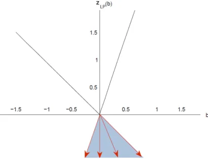
Figure 1.2: The LP value function (1.12) and the set of its subgradients at zero.

Example 1.2. The dual problem of an instance of (1.12) when bis fixed to ˆb is

sup ˆbν

s.t. ν ≤4 2ν ≤6

−7 ν ≤7

(1.19)

The extreme points of the feasible region of the dual problem above are −1 and 3. The functionzLP is plotted in Figure 1.2. As one can observe, this function is differentiable everywhere except at b = 0. The gradient of the function at a given point ˆb ∈(−∞,0) is−1, an extreme point of the feasible region to (1.19). Similarly, the gradient of the LP value function over (0,∞) is 3. At the origin, the function is subdifferentiable and we have

∂zLP(0) =cl(conv({−1,3})).

Proposition 1.2enables us to derive polyhedral dual functions for the value function of an LP by solving the dual LP instance at a given right-hand side. For example, if the dual problem of (1.12) withb fixed at −1 is solved, from the optimal solution we derive

(28)

the dual function f(b) =−2b. If b is fixed to 4, the optimal dual solution is 0.5 and we obtain f(b) = 3b, another dual function. In the case where the right-hand sideb is fixed to zero, we can obtain a dual function from the subgradient inequalities

zLP(b)−zLP(0)≥g(b−0) =gb,

where g ∈ cl(conv({−1,3})) and zLP(0) = 0 because the feasible region of the dual problem (1.19) is non-empty.

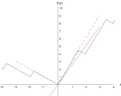
We mentioned earlier that construction of dual functions to the second-stage value function is key in classical methods of solving two-stage optimization problems. In the case of a linear second-stage problem, dual functions can be derived by obtaining subgra-dients of the value function as shown in Proposition (1.2). However, such linear functions do not give valid dual functions for the case where the second-stage problem contains in-teger variables. We show this with an example next and discuss further technical details in Chapter 2and Chapter 3.

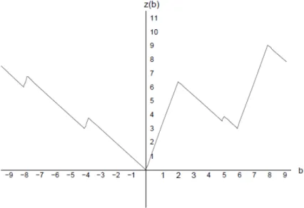
Example 1.3. Consider the MILP value function defined by adding integer variables to (1.12).

z(b) = inf 4x1+x2+ 4x3+ 6x4+ 7x5

s.t.2x1−2x2+x3+ 2x4−7x5=b x1, x2 ∈Z+, x3, x4, x5∈R+.

(1.20)

Figure 1.3shows this non-convex and non-concave function, along with the LP value function in Example1.1. The function f(b) = 2.5bis plotted in red. As one can observe in the figure, this function is a dual function for zLP (in dashed blue), but not for the MILP value functionz.

What we illustrated in the previous example in fact can be generalized: the general dual functions to the MILP value function cannot be linear functions. However, there are classes of functions that result in dual functions for the MILP value functions. We discuss these classes and review their construction methods in Chapter 2.

(29)

Figure 1.3: The MILP value function (1.20).

Benders’ Principle

Consider the linear optimization problem (1.9) where the variables are partitioned into two groups. The problem can be written equivalently as

zLP = inf c>1x1+c>2x2

s.t. A1x1+A2x2= ˜b x1∈Rp+, x2∈Rn+−p.

(1.21)

Suppose that the variablesx1 are “complicating” variables, in the sense that the problem

becomes easy to solve if these variables are fixed. The idea ofBenders’ decomposition is to partition the problem into two problems, one called themaster problemwhich contains the complicating variablesx1, the second called thesubproblem that contains the variables x2. We formulate these problems next. Let us first rewrite (1.21) as

inf x1∈Rp+

(30)

wherez0 is the LP value function

z0(˜b−A1x1) = infc>2x2

s.t. A2x2 = ˜b−A1x1 x2 ∈Rn+−p.

(1.23)

From the formulation of the dual problem of an LP in (1.16), we have that the feasible region of the dual of (1.23) does not depend on x1. Assuming that this feasible region

is non-empty, we have a representation of (1.23) in terms of its dual extreme points and directions as

z0(˜b−A1x1) = infθ (1.24)

s.t. 0 ≥(˜b−A1x1)>dj ∀j∈L (1.25) θ ≥(˜b−A1x1)>νi ∀i∈K, (1.26)

where νi with i ∈ K and dj with j ∈ L are respectively the dual extreme points and directions defined in (1.18). Therefore, the original problem (1.21) can be equivalently written as

zLP = infc>1x1+θ

s.t.0≥(˜b−A1x1)>dj ∀j∈L (1.27) θ≥(˜b−A1x1)>νi ∀i∈K, (1.28) x1 ∈Rp+.

Note that if ˜bis replaced with the parameter b, the right-hand side of each constraint in (1.28) is a dual function to the LP value function z0. That is,

(b−A1x1)>νi ≤z0(b−A1x1). ∀i∈K (1.29)

(31)

all the constraints (1.27) and (1.28) in the problem. Instead, Benders’ decomposition dynamically generates a subset of these sets in the master problem in such a way that the optimal solution is still obtained. The master problem is formulated as

zLP = inf c>1x1+θ

s.t.0≥(˜b−A1x1)>dj ∀j∈L0⊆L (1.30) θ≥(˜b−A1x1)>νi ∀i∈K0⊆K, (1.31) x1 ∈Rp+.

Benders’ decomposition algorithm starts with L0 =∅ and K0 =∅ to obtain an initial solution (ˆx1,θˆ) from the master problem. We then solve the resulting subproblem (1.23)

by fixingx1to ˆx1and obtaining a new dual extreme point or direction to form a constraint

in the form of (1.30)–(1.31). For a given ˆx1, if the dual of (1.23) is unbounded, then (1.23)

is infeasible and we can obtain an extreme direction to form a constraint in the form of (1.30). Constraints of this type are called Benders’ feasibility cuts. When the dual problem w.r.t. x1has a finite optimum andx1is not feasible, we can generate a constraint

in the form of (1.31) which is violated by x1, which are known as a Benders’ feasibility cut. These constraints are appended to the master problem, which is then resolved. The method terminates when the solution to the master problem satisfied ˆθ=z0(˜b−A1xˆ1).

That is, the approximation of the value function of the subproblem obtained from the master problem in the final iteration should coincide with the exact value function of the subproblem at the right-hand side ˜b−A1xˆ1.

Benders’ method can be applied to MILPs. In this case, the variables are normally partitioned into the sets of integer and continuous variables. The integer variables are considered the complicating variables. The assumption is that by fixing the integer vari-ables, the remaining problem is an LP that can be solved efficiently. Like the LP case, in each iteration of the Benders’ algorithm, a new dual feasible solution to the subproblem is obtained that is used to construct an optimality or feasibility constraint. Due to the integrality restriction on the complicating variables, the master problem is, however, an

(32)

integer optimization problem. In what comes next, we discuss the application of Benders’ decomposition to two-stage stochastic optimization problems.

1.3 Two-stage Stochastic Linear Optimization

Two-stage stochastic optimization problems involve decisions that are made in two points of time. The decisions made in the absence of information about the uncertainty are called thefirst-stage decisions, while the decisions made after the uncertainty is realized with the goal of correcting the initial decisions are called thesecond-stage decisions. We consider the following formulation of the two-stage stochastic mixed integer linear problem

min x∈S1

Ψ(x), (SP)

where S1 = {x ∈ Zr+1 ×Rn1 −r1

+ | Ax = b} is the first-stage feasible region defined by A∈_Qm1×n1 _and _b_∈

Qm1. The objective function Ψ is defined by

Ψ(x) =c>x+ Ξ(x), (1.32)

where c ∈ _Rn1 _{reflects the immediate cost of implementation of the first-stage solution}

and Ξ is a risk measure reflecting the additional cost incurred as a result of uncertainty about the future. As is conventional for stochastic optimization problems, we take Ξ to be the expected cost of the recourse problem, henceforth referred to as thesecond-stage problem. The second-stage problem is a MILP parameterized on both the value of the first-stage solution and a random variableω. Formally, the function Ξ is defined by

Ξ(x) =Eω∈Ω[z(hω−Tωx)], (1.33)

for x ∈ S1, where Tω ∈ Qm2×n1 and hω ∈ Qm2 represent the realized values of the stochastic inputs to the second stage for scenario ω ∈ Ω. The functionz is the second-stage value function, which encodes the cost of the recourse decision for a given first-stage solutionx and realizationω. This value function is defined earlier in (1.8). We rewrite it

(33)

in the context of the stochastic problem. For anyb∈Rm2, we have

z(b) = inf{q>y|y∈S2(b)}, (RV)

where S2(b) = {y ∈ Zr+2 ×R

n2−r2

+ | W y = b}. For a given ˆb ∈ Rm, S2(ˆb) is the second-stage feasible region with respect to ˆb, defined by constraint matrix W ∈ _Qm2×n2_{, and}

the second-stage objective functionq ∈_Rn2_{, which represents the cost of recourse action.}

In general, we may have a stochastic matrixWω and a stochastic vectorqω. In this case, one has to work with|Ω|individual second-stage value functions. Although our results on the MILP value function in Chapter2and the method we propose to solve the two-stage problem in Chapter3 remain valid in this case, we assume a fixedW andq to be able to work with a single value function in the second-stage problem. We next illustrate that the two-stage problem (SP) has a desirable structure which can be exploited in the Benders’ framework to solve these problems.

The structure of the function Ψ is closely related to the structure ofφ. The following example illustrates this.

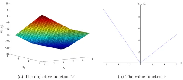
Example 1.4. Consider the following instance of a continuous two-stage problem (r1 = r2 = 0). min Ψ(x) =−3x1−3.8x2+ X ω∈Ω 0.5z(hω−2x1−0.5x2), s.t. x1 ≤5, x2 ≤5, x∈R2+, (1.34) where zLP(b) = min 6y1+ 4y2+ 3y3+ 4y4+ 5y5+ 7y6 s.t. 2y1+ 5y2−2y3−2y4+ 5y5+ 5y6 =b, y∈_R6 +, (1.35)

where Ω ={1,2},h1 = 6, h2 = 12. Figures1.4aand 1.4b show the form of the objective

function Ψ and second-stage value functionzLP, respectively, for Example1.4. Both these functions are convex and can be approximated from below by subgradient inequalities in

(34)

(a) The objective function Ψ (b) The value functionz

Figure 1.4: The objective function Ψ and second-stage value function z in Example1.4.

the form of (1.29). Note the similarities in shape of the two functions. The structure of Ψ clearly derives from that ofzLP.

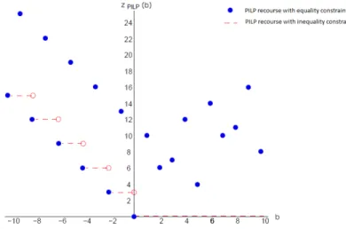
In the next example, we illustrate the form of the value function in the pure integer case for whichr2=n2.

Example 1.5. Figure 1.5 shows two value functions resulting from the addition of in-tegrality constraints to the problem of Example 1.4for all variables in the second stage. The points plotted in blue (closed circles) are the finite values of the value function of the resulting recourse problem, while the function in red (dashed lines and open circles) is the value function of the recourse problem when the single linear constraint is relaxed to the inequality 2y1+ 5y2−2y3−2y4+ 5y5+ 5y6≤b.

In the pure integer case, the discrete nature of the problem is evident in the structure of the value function, which is only finite on a discrete set of points. In the inequality form, the value function remains constant over a countable number of regions of the domain. The discrete structure of the value function in this special case has been exploited in the development of several solution methods relying on combinatorial enumeration schemes (Ahmed et al.,2004;Kong et al.,2006;Trapp et al.,2013;Schultz et al.,1998). The structure above changes substantially when we have both continuous and integer variables in the second-stage problem. Let us modify the previous example such that we

(35)

Figure 1.5: The value functions of two pure integer variations of (1.35)

have a MILP in the second-stage.

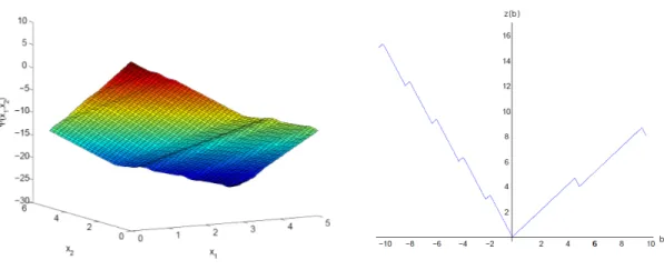
Example 1.6. Consider the mixed integer variation of Example 1.4where

z(b) = min 6y1+ 4y2+ 3y3+ 4y4+ 5y5+ 7y6

s.t.2y1+ 5y2−2y3−2y4+ 5y5+ 5y6=b y1, y2, y3 ∈Z+, y4, y5, y6∈R+.

(1.36)

Figures 1.6a and 1.6b respectively show the objective function and second-stage value function, respectively, for this mixed integer variation of the problem from Example1.4.

We discussed earlierzLP defined in (1.11) is a convex function in the continuous case. As a result, Benders’ method can be applied straightforwardly in the same fashion we de-scribed in Section1.2. This is true even with the introduction of integrality constraints in the first stage (r1 >0), as shown byVan Slyke and Wets(1969). Thus, whenr2= 0, (SP)

can be solved in principle using little modification in the Benders’ method. Whenr2 >0, zis non-convex and discontinuous in general. As Example1.6should make clear, solution methods for the more general non-convex case must either exploit special structure, such as in Example1.5, or rely on a more general class of functions for approximating the value function from below. In this thesis, we take the latter approach. To start, we need to

(36)

(a) The objective function Ψ in Example1.6. (b) The value functionzin Example1.6.

Figure 1.6: The objective and second-stage value functions for Example 1.6.

describe the Benders’ method with general lower bounding functions for the second-stage value function.

We assume ω is drawn from a given discrete and finite probability space (Ω,A, P) so that ω represents which one of a finite number of explicitly enumerated scenarios is realized andpω represents the probability of such realization. Then, (1.33) is equivalent to

Ξ(x) =X ω∈Ω

pωz(hω−Tωx). (1.37)

Therefore, the expectation in (SP) can be expressed as the sum of a finite number of terms, which allows for reformulation of (SP) as a large-scale MILP, the so-calleddeterministic equivalent problem: min c>x+X ω∈Ω pωq>yω s.t. Ax=b Tωx+W yω =hω ∀ω∈Ω x∈Zr+1×R n1−r1 + , y∈Z r2 + ×R n2−r2 + . (DE)

Figure 1.7illustrates the structure of the constraints of (DE). From this figure, one can observe that the variablexacts as a “linking” or “complicating” variable. That is, ifx is

(37)

       A T1 W . .. T|Ω| W               x y1 .. . y|Ω|        =        ˜_b h1 .. . h|Ω|       

Figure 1.7: The constraints of (DE)

fixed, the constraint matrix can be separated into|Ω|individual blocks, each consisting of the the matrixW. Consider (DE) with a fixed ˆx. The resulting problem is

min {c>xˆ+X ω∈Ω pωq>yω} s.t. W yω=hω−Tωxˆ ∀ω ∈Ω y∈_Zr2 + ×Rn2 −r2 + . (1.38)

Clearly, (SP) can be decomposed into |Ω| independent subproblems. Naturally, the majority of the methods developed to solve (SP) are decomposition based methods that take advantage of the underlying block structure of the problem. As we discussed earlier, Benders’ decomposition is designed in such a way to take advantage of the fact that the resulting problem after fixing the first-stage variables is relatively easy to solve. In this case, the remaining problem (1.38) is itself a separable problem. Due to the shape of the building blocks forming (DE)’s constraints, this method is also known as the L-shaped method. We will provide technical details of this method in Chapter 3. Here, we briefly explain the outline of the method when applied to (SP) and discuss its connection with the structure of the value function of the second-stage.

Consider (SP). We first begin by rewriting the problem (SP) as

min c>x+θ s.t. θ≥ X ω∈Ω pωz(hω−Tωx) x∈S1. (1.39)

(38)

Like the classical Benders’ method, the idea is to approximate the right-hand side of the first set of constraints in (1.39) by a set F_ω of dual functions for each scenario and to iteratively strengthen the approximation yielded by these dual functions through the generation of additional such functions. To form the master problem, we therefore replace the value function with such an approximation to obtain

min{c>x+θ|θ≥X

ω∈Ω

pωmax

f∈Fω

f(hω−Tωx)}, (1.40)

whereF_ω represents the set of all dual functions associated with scenarioωthat have been generated so far. In iteration k, a strong dual function f_ωk is produced for each scenario with respect to a proposed first-stage solutionxk∈S1, the solution to the master problem

in the previous iteration, by solving the dual problem

max

f {f(hω−Tωx

k₎_|_f₍_{W y}₎_≤_q>_y_}_. _(1.41)

The collection of dual functions is then enlarged appropriately. With this approximation, the master problem afterk iterations of the algorithm is

min c>x+θ s.t. θ≥X ω∈Ω pω max i=1,...,kf i ω(hω−Tωx) x∈S1. (1.42)

The algorithm terminates at iteration K if the solution to the master problem (x∗, θ∗) satisfies θ∗ = maxi=1,...,Kfωi(hω −Tωx∗), that is, the approximation of the expected recourse at the final iteration is exact.

It should be clear by now that applying Benders’ decomposition to the general (SP) requires constructing dual functions for MILPs. Later in Section 2.6, we discuss that in practice, we are interested in finding dual functions that can be constructed as a by-product of integer optimization algorithms to solve scenario subproblems. We study the derivation of such dual functions and provide details about incorporating them into the

(39)

Benders’ method in Sections2.6,3.3 and3.4.

1.4 Contributions

In Chapter2, we provide an in-depth review of the structure and properties of the general MILP value function. We extend previous results by demonstrating that the MILP value function has an underlyingdiscrete structuresimilar to the value function of apure integer optimization problem (PILP), even in the general case. This discrete structure emerges from separating the function into discrete and continuous parts, which in turn enables a representation of the function in terms of two discrete sets. We discuss the role of integer and continuous variables in the structure of the value function and in defining the discrete set. We provide a new representation of the value function using the discrete set and demonstrate that this representation can be applied to represent the value function of an LP and a PILP. Furthermore, we show the correspondence between the discrete set and the regions over which the MILP value function is continuous and convex. We show that the representation we provide can be constructed and propose an algorithm for doing so.

Using our earlier discrete representation of the MILP value function, we propose a deterministic reformulation of the two-stage problem in Chapter 3. We then describe a generalization of the classical Benders’ method for solving two-stage mixed integer optimization problems and demonstrate that the algorithm is convergent if strong dual functions encoded in the branch-and- bound trees that are used to solve the second-stage subproblems are employed to approximate the second-second-stage value function. We demonstrate that it is possible to solve all second-stage subproblems with a single branch-and-bound tree and to refine the approximation using this tree. Finally, we show that this procedure allows us to conclude that there exists a single branch-and-bound tree that encodes the full value function.

In Chapter 4, we propose three warm-starting strategies to apply to the Generalized Benders’ method we propose. We illustrate that each strategy leads to a different

(40)

approx-imation of the second-stage value function within the Benders’ method. We use cut-pool management techniques to keep the size of the approximation manageable. Finally, we apply the algorithm to the problems in stochastic server location test set and analyze the performance of the algorithm under different warm-starting techniques.

1.5 Outline of Thesis

Chapter 2 includes the result of our work on the value function of a mixed integer opti-mization problem. Section 2.1provides a review of duality in integer optimization. The discrete structure of the value function is examined in Section 2.2. Sections 2.3and 2.4

respectively contain our results on the structural properties of the value function and a simplification of the Jeroslow formula that we propose by using our discrete represen-tation. The proposed algorithm for construction is stated in Section 2.5. Finally, in Section2.6 we review the upper and lower bounding methods to approximate the value function.

Chapter 3 contains our contributions in solving two-stage stochastic mixed integer optimization. we review the structural properties and solution methods of the continuous two-stage stochastic problems in Section 3.1. Section 3.2 included the literature review on the algorithms for the two-stage integer optimization problems. In Section 3.3, we provide a new formulation for this problem and discuss the implication of warm-starting the constructions approximating functions for the second-stage value function. Section3.4

contains details and convergence results of the proposed algorithm to solve the two-stage mixed integer optimization problem.

We review MILP sensitivity analysis as well as the techniques to warm-start MILPs in Section4.1. We overview current warm-starting techniques implemented in the MILP solver, SYMPHONY in Section 4.2. Section 4.3 contains the implementational details of the generalized Benders’ algorithm, as well as alternative methods to construct ap-proximations of the second-stage value function and several bunching and warm-starting strategies that can be used in the algorithm. Finally, we report our computational results

(41)

obtained by applying the algorithm to problems from the literature and SIPLIB.

(42)

The Value Function of a Mixed

Integer Linear Optimization

Problem

Understanding and exploiting the structure of the value function of an optimization prob-lem is a critical eprob-lement of solution methods for a variety of important classes of multi-stage and multi-level optimization problems. Previous findings on the value function of a PILP have resulted in finite algorithms for constructing it, which have in turn enabled the development of solution methods for two-stage stochastic pure integer optimization problems (Schultz et al., 1998; Kong et al., 2006) and certain special cases of bilevel optimization problems (Bard, 1998). Studies of the value function of a general MILP, however, have not yet led to algorithmic advances. The goal of this chapter is to overview the previous work and provide new results on the structure and construction methods of the general MILP value function.

We start this section by reviewing the fundamental concepts that are necessary for the remainder of the chapter. We review MILP duality and the known results about the structure of the MILP value functions. In Section 2.2, we extend previous results by demonstrating that the MILP value function has an underlying discrete structure

(43)

similar to the PILP value function, even in the general case. We demonstrate that discrete structure emerges from separating the function into discrete and continuous parts, which in turn enables a representation of the function in terms of two discrete sets. In Section2.3, we show how this discrete structure can explain certain structural properties of the MILP value function and use our representation to characterize regions over which the value function is convex and continuous.

We review lower and upper bounding approximation methods for the MILP value function in Section2.6. Using our discrete representation, we develop an exact algorithm to construct the value function. We show this and the proof of finiteness of the algorithm in Section2.5.

In the final section of this chapter, we show how that our discrete representation can explain several previously known properties of two well-known special cases of the MILP value function: the value function of a MILP with a single constraint and the value function of a PILP.

2.1 Overview

Recall that we defined a mixed integer optimization problem in (MILP) with

z= inf x∈Sc

>

x, (MILP)

wherec∈_Rn _{is the objective function vector and} _S ₌_{_x_∈

Zr+×Rn+−r|Ax=b} is the

feasible region, described byA∈_Qm×n_,_b_∈

Rm, and a scalarr indicating the number of integer variables. We also defined the value function of a MILP in (1.8) in

z(b) = inf x∈S(b)c >_x _∀_b_∈_B, _(2.1) where for b ∈ _Rm_, _S₍_b_{) =} _{_x _∈ Zr+×Rn −r + | Ax = ˆb} and B = {b ∈ Rm |S(b) 6= ∅}.

We assumed by convention thatz(0) = 0. Let us introduce a few further notation that will be used widely in this chapter to find the discrete structure of z. We introduce

(44)

the discrete analogue to S(b) and B by letting SI(b) = {xI ∈ Zr+ : AIxI = b} and

BI ={b∈Rm :SI(b)=6 ∅}. Finally, we let SI =∪b∈B SI(b).

In Chapter1, we defined a dual function in Definition 1.1and showed that it follows from the LP duality theory that linear functions can be strong dual functions for the LP value functions. In what comes next, we overview major results in the duality theory for integer optimization problems. Mainly, we introduce certain classes of functions that can be used as dual functions for the MILP value function and discuss several methods for their construction.

The definition of dual functions in (1.13) is rather broad and does not impose a particular structure on the dual function. When dual functions are used within solution methods, such as the Benders’ method we discussed in the previous chapter, then it is desirable for the dual function to be computable in practice. We saw earlier in Chapter1

that linear functions are not dual to the MILP value function in general. The next natural class of functions to consider is convex functions.

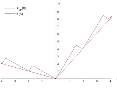
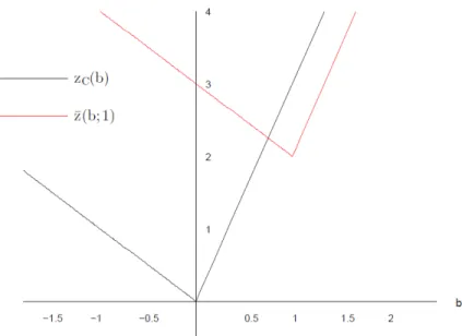
The Subadditive Dual Let us once more consider the MILP value function (1.20). In Figure2.1, the best piecewise linear convex function that is dual to the MILP is plotted along with the original value function. As one can observe in the figure, this function is strong only at the lower break points of the value function. The weak approximation provided by this convex function elsewhere is not a surprise, given that the MILP value function is non-convex and can clearly be best approximated by a non-convex function.

It turns out that the optimal convex dual function is in fact the value function of the LP relaxation of the MILP. In the case of the MILP (1.20), this problem is

zLP(b) = inf 4x1+x2+ 4x3+ 6x4+ 7x5

s.t.2x1−2x2+x3+ 2x4−7x5 =b x1, x2, x3, x4, x5 ∈R+.

(45)

Figure 2.1: The value functions (1.20) and (2.2). which is equivalent to zLP(b) = supbν s.t. −0.5≤ν ≤2 ν ∈_R. (2.3)

(2.3) can be explicitly written as

zLP(b) =      2b if b≥0 −0.5b if b <0 which is precisely the convex function plotted in Figure2.1.

Searching for candidate classes of functions,Johnson(1973) first proposed the idea of restricting to the class ofsubadditive functions.

Definition 2.1. A function f : Rn → R is called subadditive on Rn if f(x1 +x2) ≤ f(x1) +f(x2) for all x1, x2 ∈Rn such thatx1+x2 ∈Rn.

The strong motivation for considering this class is that the value function itself is a subadditive function on B. Therefore, there is always a dual function to the dual problem (1.14) that is subadditive: the value function.

(46)

Proposition 2.1. The value function (1.8) is subadditive on B.

Proof. Consider b1, b2 ∈ B. Let z(b1) = c>x1 and z(b2) = c>x2 for some x1 ∈ S(b1)

and x2 ∈ S(b2). We have (b1+b2) ∈ S(b1 +b2), therefore z(b1+b2) ≤ c>b1+c>b2 = z(b1) +z(b2).

Johnson showed that for a feasible MILP, we have

infc>x Ax= ˆb x∈Zr+×Rn −r + = supF(ˆb) F(Aj)≤cj ∀j∈I ¯ F(Aj)≤cj ∀j∈C F(0) = 0, F subadditive. (2.4)

whereAj is the jth column of Aand the function ¯F is defined as

¯ F(b) =lim sup δ→0+ F(δb) δ ∀b∈R m_. _(2.5)

The second problem is known as thesubadditive dual problem.

Definition 2.2. The directional derivative of a function f :Rn → R in the direction p at point x0 is given by

f0(x0, p) = lim

h→0

f(x0+hp)−f(x0)

h .

In the case the limit exists, the function is called directionally differentiable atx0 in the

directionp.

The directional derivative gives the rate of change of the function, moving through

x0 in a given direction pand provides a useful characterization when the function is not

continuously differentiable atx0. The function ¯F is the upper d-directional derivative of F at zero, first introduced by Gomory and Johnson (1972a,b). Intuitively, ¯F provides an upper bound to F near zero and ensures that a function that is feasible to (2.4) has

(47)

Figure 2.2: The upper d-directional derivative of (1.20).

gradients that do not exceed the gradients of the value function near zero. This was formally shown in a subsequent paper byJohnson(1974).

Proposition 2.2. If F is a subadditive function with F(0) = 0, then for any b ∈ _Rm

withF¯(b)≤ ∞ and any λ≥0, we haveF(λb)≤λF¯(b).

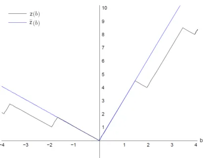
Example 2.1. Consider the MILP value function (1.20). This function and its upper d-directional derivative ¯z are plotted in Figure 2.2, where ¯z is defined as

¯ z(b) =      3b if b≥0 −b if b <0

The function ¯z is an upper bounding function to z near zero. One may note that this function is identical to the value function of the LP (1.1), which consists of only the continuous variables of the MILP. We show that this is not a coincidence and provide further details on it in Section2.2.

Subadditve dual functions are extremely important to the theory of duality for MILPs. Subadditive dual functions not only provide lower bounds for the MILP instance with the

(48)

right-hand side ˆb, but also they allow to carry over several properties of the LP duality to the MILP case such as strong and weak duality and complementary slackness. We state these results next.

Theorem 2.1. (weak duality byJeroslow (1978, 1979)) If F is a feasible solution to the subadditive dual problem (2.4) and xˆ is a feasible solution to (MILP) with its right-hand side fixed atˆb∈B, then F(ˆb)≤c>xˆ.

Proof. Consider an arbitrary ˆb∈B and ˆx such that ˆx∈S(ˆb). From the subadditivity of

F we have F(ˆb) =F(Axˆ)≤F(X j∈I Ajxˆj) +F( X j∈C Ajxˆj). (2.6)

Since F(0) = 0 and xj ∈Z+ for all j∈I and F is subadditive, we have

F(X j∈I Ajxˆj)≤ X j∈I F(Aj)ˆxj. (2.7)

Similarly, since ¯F(0) = 0, and F(Ajxj) ≤ F¯(Aj)xj for xj ∈ R+, j ∈ C, and F is

subadditive we have F(X j∈C Ajxˆj)≤ X j∈C ¯ F(Aj)ˆxj. (2.8) Together, we have F(b)≤X j∈I F(Aj)ˆxj+ X j∈C ¯ F(Aj)ˆxj ≤cx,ˆ (2.9)

where the last inequality holds since we have F(Aj) ≤cj, j ∈ I and ¯F(Aj) ≤ cj, j ∈ C by feasibility ofF for the subadditive dual problem and xj ≥0 by its feasibility for the primal MILP.

The proof of the strong duality and complementary slackness require some extra machinery which we will not provide here for the sake of space and refer to the original texts in (Jeroslow,1978,1979;Johnson,1974). The next result addresses the necessary and sufficient conditions on the infeasibility and unboundedness of the primal and dual problems. These results are analogous to those in LP duality.

(49)

Proposition 2.3. The following statements hold for the primal problem (MILP) and its subadditve dual problem (2.4).

i (MILP) is unbounded if and only if b∈B and z(0)≤0. ii The dual problem is infeasible if and only if z(0)<0.

iii If the primal problem (respectively, the dual) is unbounded, then the dual problem (respectively, the primal) is infeasible.

iv If the primal problem (respectively, the dual) is infeasible, then the dual problem (re-spectively, the primal) is infeasible or unbounded.

Next, we state the strong duality theorem for MILPs, which is due toJeroslow(1978,

1979).

Theorem 2.2. (strong duality) If either the primal problem (MILP) or the dual problem

(2.4) has an optimal value, then there exists an optimal feasible solutionx∗ to the primal problem and an optimal dual functionF∗ to the dual problem for which c>x∗=F∗(b).

Finally, we arrive at the complementary slackness result. Complementary slackness is a significant result as it provides a certificate of optimality for the primal-dual pair (MILP) and (2.4).

Theorem 2.3. (Jeroslow,1978, 1979; Bachem and Schrader, 1980) Letx∗ be a feasible solution to (MILP) with its right-hand side fixed at a given ˆb and F∗ be an optimal solution the subadditive dual problem (2.4). Then, x∗ and F∗ are optimal if and only if

x∗_j(cj−F∗(Aj)) = 0, ∀j∈I

x∗_j(cj−F¯∗(Aj)) = 0, ∀j∈C.

(2.10)

Although the stated results provide the theoretical fundamentals and answer several important questions about duality of integer optimization problems, we still need to find methods to compute and encode dual functions for MILPs. We review some methods to construct feasible, and in some cases optimal, dual functions in section2.5.

(50)

The Chv´atal Representation Blair and Jeroslow(1982) first showed that the value function of a PILP is a Gomory function that can be derived by taking the maximum of finitely many subadditive functions. In a subsequent work, they extended their earlier results in (Blair and Jeroslow,1984) and identified a subclass of Gomory functions called

Chv´atal functions to which the general MILP value function belongs.

Definition 2.3. TheGomory functions are the smallest class Gm of functions such that i For anyα∈Qm,f(b) =αbis inGm.

ii If f1, f2 ∈Gm and α, β∈Qm+, then αf1+βf2 ∈Gm.

iii Iff ∈Gm_{, then}_d_f_{e ∈}_Gm_.

iv If f1, f2 ∈Gm, then max{f1, f2} ∈Gm.

The Ch´avatal functions are the smallest class satisfying i–iii.

The following two results show the connection between Gomory and Chv´atal functions and that both of the classes have the subadditivity property.

Proposition 2.4. (Blair and Jeroslow, 1982) If g is a Gomory function, then there is a finite number of Chv´atal functions f1, . . . , fN such that

g= max{f1, . . . , fN}. (2.11)

Proposition 2.5. (Blair and Jeroslow, 1982) Any Chv´atal or Gomory function is sub-additive.

The main results that address the connection between the PILP and MILP value functions and Gomory and Chv´atal functions are Theorems2.4 and 2.6. First, we state the lemmas needed for the main results. The first lemma below shows that the convex hull ofS can be represented by subadditive functions and this representation is finite for the case of a PILP.

(51)

Lemma 2.1. (Blair, 1978; Bachem and Schrader, 1980;Wolsey,1981b) For any b∈B we have conv(S(b)) ={x∈_Rn₊|X j∈I F(Aj)xj+ X j∈C ¯ F(Aj)xj ≥F(b), F subadditive, F(0) = 0}. (2.12)

In the case of a PILP, there exist finitely many subadditive functionsFi, i= 1, . . . , ksuch

that

conv(S(b)) ={x∈_Rn₊|X

j∈N

Fi(Aj)xj ≥Fi(b), i= 1, . . . , k}. (2.13)

Knowing that subadditive functions can represent the convex hull of solutions to PILPs and that Chv´atal functions are subadditive, Schrijver (1980) showed that for PILPs, Chv´atal functions can in fact be used to represent the convex hull of solutions. We state this lemma first and use it to arrive at Theorem 2.4, which shows that every value function of a PILP can be represented as a Gomory function.

Lemma 2.2. (Schrijver, 1980) The subadditive functions in (2.13) can be taken to be Chv´atal function.

This lemma is used to represent the value function of a PILP as a Gomory function. Theorem 2.4. (Blair and Jeroslow,1982) There always exists a Gomory functiongsuch thatg(b) =z(b) for all b∈B, where z is the value function of a PILP with z(0) = 0.

It is worth noting that for any Gomory function g, there is always a PILP such that

g coincides with the value function of the PILP. We state this formally next.

Theorem 2.5. (Blair and Jeroslow,1986) Consider (MILP) withC=∅. Then, for any Gomory function g there are A andc such that g(b) is the optimal objective value to the problem for all vectors b∈B.

Subsequently, Blair and Jeroslow (1984) extended their results from the PILP to the MILP case by showing that every MILP value function is a minimum of finitely many Gomory functions.