ePrints Soton
Copyright © and Moral Rights for this thesis are retained by the author and/or other
copyright owners. A copy can be downloaded for personal non-commercial
research or study, without prior permission or charge. This thesis cannot be
reproduced or quoted extensively from without first obtaining permission in writing
from the copyright holder/s. The content must not be changed in any way or sold
commercially in any format or medium without the formal permission of the
copyright holders.
When referring to this work, full bibliographic details including the author, title,
awarding institution and date of the thesis must be given e.g.
AUTHOR (year of submission) "Full thesis title", University of Southampton, name
of the University School or Department, PhD Thesis, pagination
FACULTY OF ENGINEERING, SCIENCES AND MATHEMATICS School of Engineering Sciences
Aerodynamics and Flight Mechanics Research Group
Unsteadiness in
shock-wave/boundary-layer interactions
by
Emile Touber
Thesis for the degree of Doctor of Philosophy
ABSTRACT
FACULTY OF ENGINEERING, SCIENCES AND MATHEMATICS SCHOOL OF ENGINEERING SCIENCES
Doctor of Philosophy
UNSTEADINESS IN SHOCK-WAVE/BOUNDARY-LAYER INTERACTIONS by Emile Touber
The need for better understanding of the low-frequency unsteadiness observed in shock wave/turbulent boundary layer interactions has been driving research in this area for several decades. This work investigates the interaction between an impinging oblique shock and a supersonic turbulent boundary layer via large-eddy simulations. Special care is taken at the inlet in order to avoid introducing artificial low-frequency modes that could affect the interaction. All simulations cover extensive integration times to allow for a spectral analysis at the low frequencies of interest. The simulations bring clear evidence of the existence of broadband and energetically-significant low-frequency oscillations in the vicinity of the reflected shock, thus confirming earlier experimen-tal findings. Furthermore, these oscillations are found to persist even if the upstream boundary layer is deprived of long coherent structures.
Starting from an exact form of the momentum integral equation and guided by data from large-eddy simulations, a stochastic ordinary differential equation for the reflected-shock foot low-frequency motions is derived. This model is applied to a wide range of input parameters. It is found that while the mean boundary-layer properties are important in controlling the interaction size, they do not contribute significantly to the dynamics. Moreover, the frequency of the most energetic fluctuations is shown to be a robust feature, in agreement with earlier experimental observations. Under some assumptions, the coupling between the shock and the boundary layer is mathematically equivalent to a first-order pass filter. Therefore, it is argued that the observed low-frequency unsteadiness is not necessarily a property of the forcing, either from upstream or downstream of the shock, but simply an intrinsic property of the coupled dynamical system.
Abstract i List of Figures vi List of Tables ix Declaration of Authorship x Acknowledgements xi Abbreviations xii Symbols xiv 1 Introduction 1 1.1 Motivation . . . 1
1.2 Introduction to the SBLI issue . . . 3
1.3 Known facts on SBLI . . . 6
1.4 Current speculations on the low-frequency unsteadiness in SBLI . . . 11
1.4.1 Correlations with upstream events . . . 11
1.4.1.1 Fast timescales . . . 11
1.4.1.2 Slow timescales . . . 13
1.4.2 Correlations with downstream flow features . . . 16
1.4.3 Objectives and thesis outline . . . 18
2 Governing equations and numerical method 20 2.1 Governing equations . . . 20
2.1.1 The Navier–Stokes equations: DNS formulation . . . 20
2.1.2 The Navier–Stokes equations: LES formulation . . . 21
2.1.2.1 Convolution filter: definition . . . 22
2.1.2.2 Application of the filter to the governing equations . . . . 24
2.1.2.3 The compressible shear-layer approximation . . . 25
2.1.3 The closure problem . . . 27
2.1.3.1 The SGS stress tensor . . . 27
The Dynamic Smagorinsky eddy viscosity model . . . 28
The Mixed-Time Scale eddy viscosity model . . . 30
2.1.3.2 The SGS heat flux . . . 30
2.1.4 Final problem formulation and numerical approach . . . 31
2.2 Boundary conditions . . . 32 ii
2.2.1 Wall, top and outflow boundary conditions . . . 32
2.2.2 The inlet boundary condition issue . . . 32
2.2.2.1 Mean inflow profiles . . . 36
Mean velocity profile in the van Driest coordinate system . 36 Mean velocity, temperature and density profiles . . . 38
Mean profile for the wall-normal component of the velocity 39 2.2.2.2 Fluctuations . . . 40
Added perturbations: the synthetic turbulence approach . . 40
Inner-layer modes . . . 41
Outer-layer modes . . . 42
The equations at glance and the parameter values . . . 42
Added perturbations: the digital filter approach . . . 44
2.2.2.3 Test on a flat plate turbulent boundary layer . . . 48
3 Validation of the numerical strategy 53 3.1 Flow conditions and numerical settings . . . 53
3.2 Comparison with PIV data . . . 55
3.3 Grid-refinement, domain- and subgrid-scale-sensitivity study . . . 59
4 Time-averaged flow-field characteristics 64 4.1 Description of the UFAST project . . . 64
4.2 Case by case comparisons . . . 66
4.2.1 The IUSTI case . . . 66
4.2.2 The ITAM case . . . 75
4.2.3 The TUD case . . . 79
4.3 Cross comparisons . . . 84
4.4 Mixing-layer properties . . . 90
5 Linear-stability analysis 97 5.1 Description of the method . . . 97
5.2 Results . . . 98
6 Unsteady aspects 103 6.1 Wall-pressure data analysis . . . 104
6.1.1 Narrow-span case and experimental results . . . 104
6.1.2 Short-signal length effects . . . 112
6.1.3 Upstream influence and digital filter . . . 115
6.1.4 All three large-span LES . . . 118
6.2 Additional cross comparisons and 3D aspects . . . 121
6.2.1 The ITAM case . . . 121
6.2.2 Probability of separation . . . 125
6.2.3 Narrow-span vs large-span LES . . . 126
6.2.4 Formation of large cells within the interaction . . . 130
6.3 Shock motions and conditional averages . . . 136
6.3.1 Detection of the shock location . . . 136
6.3.2 Some characteristics of the shock motions . . . 137
6.3.3 Conditional averages . . . 141
7 Low-order stochastic model 149
7.1 Derivation of model equations . . . 150
7.1.1 Initial form of the momentum integral equation . . . 150
7.1.2 Change of variable . . . 151
7.1.3 Approximate form of the momentum integral equation . . . 153
7.1.4 Hypothesis of the existence of a similarity solution . . . 155
7.1.5 Leading-order equations . . . 158
7.2 Modelling the ODE coefficients . . . 162
7.2.1 The k coefficient . . . 162
7.2.2 The Θi coefficients . . . 165
7.2.3 The κp and κ2 coefficients . . . 168
7.3 Final form of the model . . . 171
7.4 Solutions to the derived stochastic model . . . 172
7.4.1 Solution to white noise: shock-foot and pressure spectra . . . 172
7.4.2 Solution for forcing by synthetic turbulence . . . 174
7.5 Model performances and discussion . . . 175
7.5.1 Model results compared with LES and experimental findings . . . 175
7.5.2 Cutoff-frequency map and sensitivity to the model constants . . . 177
7.5.3 Discussion and implications with respect to the low-frequency unsteadiness . . . 181
8 Conclusion 185 A Filtering the Navier–Stokes equations 190 B Fortran routine to generate the mean inflow profiles 193 C Digital-filter Fortran routines 197 C.1 Main digital-filter routine . . . 197
C.2 Some of the common arrays and parameters used . . . 204
C.3 Dependent subroutines . . . 210
D Matlab/Fortran scripts to extract the shock system 216 D.1 Step 1. Extraction from the raw data . . . 216
D.2 Step 2. Compute mean position . . . 220
D.3 Step 3. Select the data range to clip . . . 222
D.4 Step 4. Clip the extracted data . . . 223
D.5 Step 5. Remove most of the spurious points . . . 228
E Proof of the phase- and conditional-average relationships inherited from hypothesis 6.1 231 E.1 Proof of corollary 6.1 . . . 231
E.2 Proof of corollary 6.2 . . . 232
E.3 Estimation of the phase-fluctuation stress tensor . . . 233
G Series expansions of the oblique-shock relations 239 G.1 Expansion of sin2(ι+θ) . . . 239 G.2 Expansion of p3/p1 . . . 241 G.3 Expansion of ρ3/ρ1 . . . 242 G.4 Expansion of M3/M1 . . . 242 G.5 Expansion of ρ3u3(1−u3/u1)/(ρ1u1) . . . 243 Bibliography 245
1.1 Concorde on final at LHR airport . . . 2
1.2 Photograph of a bullet in supersonic flight . . . 2
1.3 Sketch of the oblique shock / boundary-layer interaction . . . 3
2.1 Discretised top-hat filter . . . 23
2.2 Spectrum of ̺k(t) obtained from (2.69) usingIx=δ0 and ¯u= 0.6¯u1 . . . 46
2.3 Skin-friction evolution: digital filtervs synthetic turbulence . . . 50
2.4 Velocity profiles: digital filtervs synthetic turbulence . . . 50
2.5 Turbulence intensities: digital filter vs synthetic turbulence . . . 51
2.6 Turbulence intensities: digital filter vs synthetic turbulence . . . 51
3.1 Mean streamwise velocity: PIVvs LES . . . 56
3.2 Mean wall-normal velocity: PIVvs LES . . . 56
3.3 RMS of the streamwise velocity fluctuations: PIV vs LES . . . 57
3.4 RMS of the wall-normal velocity fluctuations: PIVvs LES . . . 58
3.5 Reynolds shear stress: PIV vs LES . . . 58
3.6 Skin-friction sensitivity to the grid resolution and domain width . . . 60
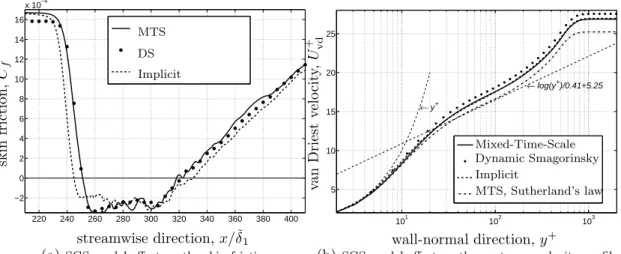
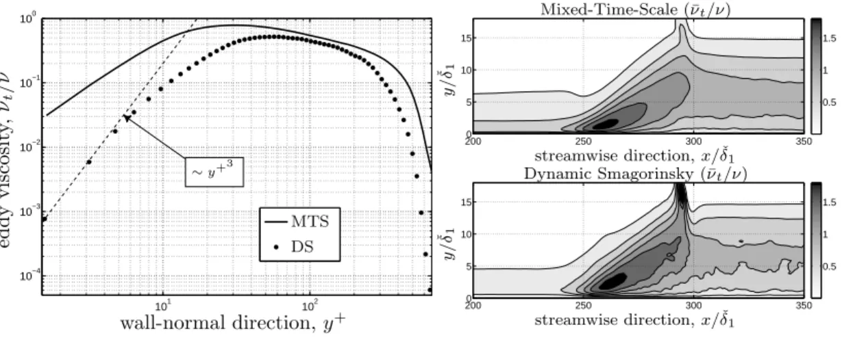
3.7 Wall pressure sensitivity to the domain width and the subgrid-scale model 61 3.8 SGS model effect on the interaction length and upstream velocity profile . 62 3.9 SGS model effect on the eddy viscosity to kinematic viscosity ratio . . . . 63
4.1 Instantaneous side views of the temperature field from the present LES . 66 4.2 IUSTI upstream velocity profiles . . . 68
4.3 IUSTI upstream Reynolds stress profiles . . . 68
4.4 IUSTI mean streamwise velocity field: LES vs PIV . . . 69
4.5 IUSTI mean wall-normal velocity field: LESvs PIV . . . 69
4.6 IUSTI streamwise-velocity fluctuation field: LES vs PIV . . . 70
4.7 IUSTI wall-normal-velocity fluctuation field: LESvs PIV . . . 70
4.8 IUSTI Reynolds shear-stress field: LES vs PIV . . . 71
4.9 IUSTI mean streamwise velocity field: LES vs PIV (2006) and PIV (2008) 71 4.10 IUSTI wall-pressure distribution . . . 72
4.11 IUSTI wall-pressure fluctuations distribution . . . 73
4.12 IUSTI mean zero-u-velocity contours . . . 74
4.13 IUSTI spanwise energy spectra: large- vs narrow-span LES . . . 75
4.14 ITAM case upstream velocity profiles . . . 76
4.15 ITAM case upstream streamwise velocity fluctuations . . . 77
4.16 ITAM wall-pressure distribution . . . 77
4.17 ITAM skin-friction distribution . . . 78 vi
4.18 ITAM LES pressure field vs Schlieren picture . . . 79
4.19 TUD upstream velocity profiles . . . 80
4.20 TUD upstream Reynolds stresses . . . 81
4.21 TUD mean streamwise velocity field: PIV vs LES . . . 82
4.22 TUD mean wall-normal velocity field: PIV vs LES . . . 82
4.23 TUD streamwise velocity fluctuations field: PIV vs LES . . . 83
4.24 TUD wall-normal velocity fluctuations field: PIV vs LES . . . 83
4.25 TUD Reynolds shear-stress field: PIV vs LES . . . 84
4.26 LES reference profiles of the UFAST cases . . . 85
4.27 LES reference Reynolds-stress profiles of the UFAST cases . . . 85
4.28 LES mean skin-friction distributions of the UFAST cases . . . 86
4.29 LES mean wall-pressure distributions of the UFAST cases . . . 87
4.30 LES mean zero-streamwise-velocity contours of the UFAST cases . . . 88
4.31 Interaction lengths vs wall-shear stress to pressure jump ratios . . . 89
4.32 Shear-layer centreline location . . . 91
4.33 Velocity profiles along the shear-layer centreline . . . 92
4.34 Shear-layer properties needed in the model by Piponniau et al. (2009) . . 93
4.35 LES shear-layer spreading rates . . . 94
5.1 Disturbances exponential growth . . . 99
5.2 Global-mode amplitude function for the streamwise momentum disturbance100 5.3 Global-mode growth rates for different spanwise wavenumbers . . . 100
5.4 Global-mode effect on the separation bubble . . . 101
6.1 Wall-pressure time signals: experimental and numerical . . . 104
6.2 Spectral analysis of the wall-pressure signals: experimentvs LES . . . 107
6.3 Energetically significant frequencies as found in the wall-pressure signals . 109 6.4 Existence of a phase jump in the wall-pressure fluctuations . . . 111
6.5 Numerical hot-wire signals . . . 113
6.6 Autocorrelation functions obtained from numerical hot wires . . . 113
6.7 Effect of short-length signals on the low-frequency analysis . . . 115
6.8 Instantaneous snapshot of u′/u¯1 . . . 116
6.9 Reconstructed u′/u¯ 1 field from a numerical transverse wire . . . 117
6.10 Inlet and upstream correlation function for long time lags . . . 117
6.11 Wall-pressure autocorrelation functions of all the UFAST cases . . . 119
6.12 Build-up of significant low-frequency oscillations for all UFAST cases . . . 121
6.13 Wall-pressure frequency/wavenumber diagrams of all the UFAST cases . . 122
6.14 ITAM LES and experimental correlation functions of the shock motions . 123 6.15 Shock-foot probability density function . . . 124
6.16 Probabilities of separation . . . 126
6.17 Narrow-span vs large-span wall-pressure spectra . . . 127
6.18 Wall-pressure dispersion relations: narrow-span vs large-span LES . . . . 128
6.19 Time series of the reversed mass-flow rate . . . 131
6.20 Tracking pockets of reversed flow . . . 133
6.21 Meandering effect on the ˙m spectrum . . . 133
6.22 Descriptive sketch of some recognisable patterns in flow animations . . . . 135
6.24 Instantaneous side view of the interaction and shock-system detection . . 137
6.25 Shock-foot probability density function . . . 138
6.26 PSD and dispersion relations of the reflected-shock transverse waves . . . 140
6.27 Shock-foot-displacement time series . . . 141
6.28 Conditional averages of the shock system: narrow-span vs large-span LES 143 6.29 Kinetic-energy fields: all vs phase fluctuations . . . 146
6.30 Shear-stress fields: all vs phase fluctuations . . . 146
7.1 Sketch of the interaction with the definition of the notations in use . . . . 151
7.2 Momentum-integral equation budget . . . 154
7.3 Validity of hypothesis 7.1 from the conditionally-averaged LES data . . . 156
7.4 Dependency of ∆i on η, relation betweensand η . . . 157
7.5 Relationship between ¯Cf0 + ˜Cf0 andζ =ε/L . . . 159
7.6 Sketch of the interaction with the notations used to compute k . . . 163
7.7 Mean pressure and momentum-thickness-integrand fields . . . 166
7.8 Validity of the Crocco–Busemann equation . . . 167
7.9 Integrands of δp andδ2 at ξ = 1 . . . 170
7.10 Spectra from the model for different forcing . . . 176
7.11 Weighted spectra from the model vs the LES and experimental results . . 177
7.12 Predicted most energetic low frequency φmax for different (M1, θ) pairs . . 178 7.13 Sensitivity of the predicted φmax map to variations in the model constants 180
2.1 Classification of the subgrid scale terms . . . 26
2.2 Parameters used for the synthetic turbulence inflow conditions . . . 43
2.3 Digital Filter coefficients . . . 48
2.4 Numerical details for the turbulent-boundary-layer simulations . . . 49
3.1 Numerical details for the grid sensitivity study . . . 54
3.2 Numerical details for the domain and SGS model sensitivity study . . . . 55
3.3 Interaction lengths and normalised shock intensity . . . 61
4.1 UFAST experimental and numerical flow conditions . . . 65
4.2 UFAST simulation settings . . . 67
6.1 Numerical details for the low-frequency study . . . 105
7.1 Amplitudes of all the constituents found in (7.23) for M1 = 2.3 andθ= 8◦161 7.2 Sensitivity of the model . . . 179
I, Emile Touber, declare that the thesis entitled “Unsteadiness in shock-wave/boundary-layer interactions” and the work presented in the thesis are both my own, and have been generated by me as the result of my own original research. I confirm that:
this work was done wholly or mainly while in candidature for a research degree at
this University;
where any part of this thesis has previously been submitted for a degree or any
other qualification at this University or any other institution, this has been clearly stated;
where I have consulted the published work of others, this is always clearly attributed;
where I have quoted from the work of others, the source is always given. With the
exception of such quotations, this thesis is entirely my own work;
I have acknowledged all main sources of help;
where the thesis is based on work done by myself jointly with others, I have made
clear exactly what was done by others and what I have contributed myself;
parts of this work have been published as: Touber and Sandham (2008a,b, 2009a,b,c,d)
Signed:
Date:
The author would like to acknowledge the UK Turbulence Consortium EP/D044073/1 for the computational time provided on both the HPCx and HECToR facilities, the UKs national highperformance computing service, which is provided by EPCC at the University of Edinburgh and by CCLRC Daresbury Laboratory, and funded by the Office of Science and Technology through EPSRCs High End Computing Program. I am also grateful to the University of Southampton for the access to its high-performance computer, Iridis2. In addition, I would like to acknowledge the financial support of the European Union through the Sixth Framework Program with the UFAST project. Finally, I am grateful to the UFAST-project partners for kindly making their data available and to both Prof. N. D. Sandham and Dr. G. N. Coleman for their guidance.
BL Boundary Layer
CTA ConstantTemperatureAnemometry
DF Digital Filter
DNS Direct NumericalSimulation
DS Dynamic Smagorinsky eddy viscosity model
FTT Flow ThroughTime
HWA Hot Wire Anemometry
ITAM Institute of Theoretical and AppliedMechanics
IUSTI Institut Universitaire desSyst`emesThermiquesIndustriels
LES Large-Eddy Simulation
LHS Left-Hand Side
MIE MomentumIntegral Equation
MTS Mixed-Time-Scale eddy viscosity model
ODE OrdinaryDifferentialEquation
PDF Probability Density Function (sometimes written pdf)
PIV Particle Image Velocimetry
PSD PowerSpectral Density
RANS Reynolds-Averaged Navier–Stokes
RDT Rapid DistortionTheory
RHS Right-Hand Side
RMS Root Mean Square
SBLI Shock-Wave/Boundary-Layer Interaction
SGS SubGrid Scale
SOTON University of SOuthampTON SRA Strong Reynolds Analogy
ST Synthetic Turbulence
TBL TurbulentBoundary Layer
TUD Delft University of Technology
TVD Total Variation Diminishing
UAN A.N. Podgorny Institute for Mechanical Engineering
UFAST EU project, see: http://www.ufast.gda.pl/ URANS Uunsteady Reynolds-Averaged Navier–Stokes
VD van Driest
A parameter in section 7.3
Aε0,∆σ set of instants, see (6.2a)
A0 parameter, q[L/(¯u1φ)]2
B parameter in section 7.3
C Sutherland’s law constant, S/T¯1,
or a parameter in section 7.3 (see context)
Cf skin friction, 2τw/(¯ρ1u¯21)
Cf0 skin friction at reflected-shock foot
CM MTS model constant, 0.03
CT MTS model constant, 10
c speed of sound
D parameter in section 7.3
D compact subset of theR3 space
Et total energy
˘
Et resolved total energy
F similarity thickness function, [δi(ξ)−δi(ξ= 0)]/∆i, see (7.10) F′ derivative ofF, dF/dξ
f frequency
fc cutoff frequency
G, G∗ convolution kernels
H reflected-shock mean and instantaneous shock-crossing point height, see figure 7.6
h time-averaged zero streamwise velocity contour height or instantaneous shock-crossing height (see context)
h0 time-averaged shock-crossing height (see figure 7.1)
K streamwise distance between the time-averaged reflected-shock foot and the reflected-shock mean and instantaneous shock-crossing point, see figure 7.6
k linear-dependence coefficient ofson ε, s/ε
kes SGS kinetic energy in the MTS model
kx stream-wise wavenumber
kξr wavenumber in the reflected-shock direction
L interaction length, ¯x0−x¯imp
Lx, Ly, Lz streamwise, wall-normal and spanwise domain length
Lsep separation length, ¯xat−x¯sep
l0 streamwise distance between the mean shock-foot and shock-crossing
positions (see figure 7.1)
M Mach number (flow-velocity to speed-of-sound ratio)
M momentum-thickness integrand, ρu[1−u/u¯1]/[¯ρ1u¯1]
˙
m reversed mass flow rate per unit width, see (6.1)
N number of periods covered by a sine wave atf = 0.035¯u1/L Nx, Ny, Nz streamwise, wall-normal and spanwise number of grid points N measure of the setAε0,∆σ, see (6.2b)
Pr Prandtl number (viscous to thermal diffusion rates ratio), 0.72 Prt turbulent Prandtl number, 1.0
P0 stagnation pressure
P2 ratiop+2/p¯1
P3 ratio ¯p3/p1¯
p pressure
q proportionality coefficient in (7.54b), or variance ofCf′′0 in (7.60)
q conservative-variable vector, [ρ, ρu, ρv, ρw, ρEt]T
R parameter in (7.45)
Ra auto-correlation function, Ra(τ) =a′(t0)a′(t0+τ)/a′(t0)a′(t0)
Reδˇ1 Reynolds number based on the code reference length, ¯ρ1u¯1δˇ1/µ¯1
Reδ1 Reynolds number based on the displacement thickness, ¯ρ1u1δ1¯ /µ1¯
Reδ2 Reynolds number based on the momentum thickness, ¯ρ1u¯1δ2/µ¯1
Reτ Reynolds number based on the friction velocity, ¯ρ1uτδ0/µ¯1 R3 ratio ¯ρ3/ρ¯1
r, r′, r′′ model coefficients, see section 7.3
r0 timescale ratio, tf/ts
S Sutherland’s temperature, 110.4 K
S power-spectral-density function
Sij strain-rate tensor, (∂ui/∂xj+∂uj/∂xi)/2 Sij∗ deviatoric part of the strain-rate tensor
Sp wall-pressure power-spectral-density function St Strouhal number,f Lsep/u1¯ orf L/u1¯ (see context)
s mean to instantaneous shock-crossing points streamwise distance
T total temperature, or a time interval (see context)
Taw adiabatic wall temperature
Tc temperature computed using the Crocco-Busemann relation
TS MTS-model timescale
Tsim simulation runtime
¯
T1 freestream total temperature upstream of the interaction
T0 stagnation temperature
t time
t⋆ normalised time,tu¯
1/L
tf timescale associated with upstream turbulence structures,δ0/u1¯ ts timescale associated with the low-frequency shock motions
t0 a chosen startup time
Uvd+ mean van Driest velocity profile in friction-velocity units
u, v, w stream-wise, wall-normal and span-wise velocity
uc convection velocity (see context for details)
¯
u1 freestream velocity upstream of the interaction
uτ friction velocity,
p
(µw/ρw)[∂u/∂y]w
x, y, z stream-wise, wall-normal and span-wise direction ¯
xat mean boundary-layer-reattachment location
¯
ximp mean location of the extension of the impinging shock to the wall
¯
¯
x0 mean location of the extension of the reflected shock to the wall
Greek
α time-averaged reflected-shock angle (see figure 7.1)
β incident-shock angle or span-wise wave-number, 2π/λz (see context) βy grid-stretching parameter in the wall-normal direction
Γ Langevin force in (7.54a)
γ specific-heat ratio, 1.4
∆i thickness amplitude function,δi(ξ= 1)−δi(ξ= 0), see (7.10)
∆t time step
∆x,∆y,∆z local grid spacing (stream-wise, wall-normal and span-wise direction) ∆,∆b,∆b filter cutoff lengthscale
δ Dirac function
δ0 boundary-layer 99% thickness
δ0imp boundary-layer thickness at the incident-shock impingement location in the absence of the shock
δ1 displacement thickness,R0h[1−ρu/(¯ρ1u¯1)] dy, h > δ0
δ1imp boundary-layer displacement thickness at the incident-shock impingement location in the absence of the shock
ˇ
δ1 inlet boundary-layer displacement thickness based on the
van Driest velocity profile using the incompressible definition
δ2 momentum thickness,R0h[ρu/(¯ρ1u¯1)] (1−u/u¯1) dy, h > δ0
δp pressure thickness,
Rh
0 [1−p/ph] dy, h > δ0 δρ density thickness,R0h[1−ρ/ρh] dy, h > δ0
ε reflected-shock foot displacement with respect to its mean position ˙
ε reflected-shock foot velocity, dε/dt
ζ normalised reflected-shock foot displacement,ε/L
˙
ζ speed of the normalised reflected-shock foot displacement, dζ/dt⋆ η vertical displacement of the shock-crossing point,h−h0 (see figure 7.1) ηr reflected-shock displacement with respect to its mean position
θ wedge angle
ϑ velocity component in the reflected-shock normal direction
ι instantaneous reflected-shock angle (see figure 7.6)
κi linear-dependence coefficient of ∆i on η, [∆i−Θi]/η
κ von Karman constant (assumed to be 0.41)
κ (tanα+ tanβ) sin (2α) sin [2 (α+θ)]/(tanβ(1−1/tanα)−1)
Λ linear-dependence coefficient of ˜Cf0 on ζ, ˜Cf0/ζ
λ length of a superstructure
λz span-wise wavelength
µ dynamic viscosity
¯
µ1 freestream dynamic viscosity upstream of the interaction
ν kinetic viscosity,µ/ρ
νt eddy viscosity
ξ moving coordinate system, (x+l0−ε)/(l0−ε+s)
¯
ξ normalised streamwise axis, (x−x¯0)/L ξr longitudinal position along the reflected shock ξ′ normalised streamwise axis, (x−x¯
sep)/Lsep
Π parameter, tanβ/[2F′(0) (tanα+ tanβ)]
π ratio of the circumference of a circle to its diameter (3.141592. . .)
̟ velocity component along the reflected-shock direction
ρ fluid density
¯
ρ1 freestream density upstream of the interaction
σ standard deviation of a signal
σij subgrid-scale stress tensor
ς component of the sound speed along the reflected-shock direction
τ correlation time
τc characteristic correlation time
τij viscous shear stress
τw time-averaged wall shear-stress,µw[∂u/∂y]w
˘
τ resolved viscous shear stress
υ steady term in (7.24)
Φ ODE damping coefficient, ¯u1φ/L
φ normalised ODE damping coefficient, see (7.26b) and (7.53b)
φmax ODE cutoff Strouhal number,φ/(2π)
ϕp disturbance phase angle with respect to a predefined reference
χ parameter, [2γ+γ(γ−1) M21]/[γ+ 1]
Ψi SGS heat flux
ψ forcing in (7.26c)
Ω power-law exponent, 0.67
ωi disturbance growth rate
Subscripts
1,2,3 the quantity is evaluated in the potential-flow region: 1 = upstream,
2 = after the incident shock but before the reflected shock,
3 = after interaction (not to confuse with vector indices, see context)
e the quantity is evaluated at the boundary-layer edge i,j,k vector index: 1 = stream-wise, 2 = wall-normal
and 3 = span-wise direction
max quantity maximum-value
min quantity minimum-value
w the quantity is evaluated at the wall
Superscripts
∗ denotes the deviatoric part of the tensor it is applied to
⋆ denotes that the dimensional variable is used
+ denotes that the variable is expressed in wall-units, y+=yu
τ/νw
and u+=u/uτ, or denotes the top side of region 2 in chapter 7
(see figure 7.1)
Operators ¯
a time-averaged or grid-filtered variable (see context) ˜
a Favre-filtered variable,ρa/ρ¯(not to confuse with the triple decomposition, see context)
a′, a′′,a˜ triple decomposition, see (6.4a) ˆ
a test-filtered variable
b ˜
a result from test-filtering the Favre-filtered variable b
¯
a result from test-filtering the grid-filtered variable
haiα α-averaged value of a
h·iε0,∆σ conditional-average operator, see (6.2c)
ˇ
a van-Driest transformed field,Ra(y=0)a(y) pρ/ρwda′
1.1
Motivation
On January 26, 1971, Concorde 001 was accomplishing its flight-test number 122 when it experienced “the most damaging incident of its development time” (Turcat, 2003). While cruising at Mach 2 over the Atlantic, upon switching off the reheat system, the third-engine-variable-inlet ramp (which can be seen in figure 1.1) was blown out due to “violent pressure fluctuations for about seven seconds”1. What Captain Defer and his crew experienced is known as inlet buzz. It is a low-frequency, high-amplitude pressure oscillation that is linked to shock-wave/boundary-layer and/or shock-wave/shock-wave interactions, affecting the engine intakes. It can seriously impair the integrity of the aeroplane, as demonstrated by Concorde 001.
According to Dolling (2001), the high-speed wind tunnel experiments on airfoils by Ferri (1940) are probably the first published observations of a shock-wave/boundary-layer interaction (SBLI). Although limited to a supersonic pocket embedded in a sub-sonic flow, additional experiments by Donaldson (1944), Liepmann (1946), Fage and Sargent (1947), Ackeret et al. (1947) quickly followed, demonstrating a sensitivity of such interactions to the state of the incoming boundary layer. However, given the pecu-liarity of the configuration (i.e. small supersonic pocket embedded in a subsonic flow with streamwise pressure gradients and surface curvature), these investigations may not have been sufficiently systematic to be conclusive.
In the late 1940’s and early 1950’s, further experiments were introduced to study the aforementioned interaction. This time, the experiments were run at fully supersonic speeds. The geometries used at that time consisted of an external shock generator, flat plate/flat ramp configurations or flat plates with steps, and axisymmetric bodies with flares/collars. Interestingly, these geometries are no different than the ones studied nowadays. These studies yielded a large data base of SBLI at various Reynolds numbers, Mach numbers and shock strengths, confirming the earlier observations of the impor-tance of SBLI and their sensitivity to the state of the incoming boundary layer. Much of that work is summarised in Holder et al. (1954). However, unlike inviscid interactions between shocks and bodies, which have already been studied for more that two centuries
1Comments by the flight observer, Claude Durand.
Figure 1.1: Concorde G-BOAE on final at LHR airport (October 10, 2003).
Photo-graph by Harm Rutten (www.airliners.net)
Figure 1.2: Photograph of a bullet in supersonic flight, published by Ernst Mach in
1887.
(see figure 1.2 and Anderson, 1990), no theory about viscous interaction is readily avail-able, particularly in the case of turbulent interactions. Thus, not equipped with such theories, researchers have run many experiments, driven by the fact that most (if not all) of the supersonic flows involve, in one way or another, a (turbulent) SBLI.
wall inciden t shock reflec ted shoc k b b b b b b b b b b b sonic line expa nsio nfa n com pre ssio nw aves flow direction relaxation separation bubble shea r lay er
Figure 1.3: Sketch of the oblique shock / boundary-layer interaction
The broad aim of the present thesis is to use the technique of large-eddy simulation to shed light on the interaction between a turbulent boundary layer and an impinging oblique shock in order to identify the flow physics and develop modelling approaches for the observed low-frequency shock motions.
1.2
Introduction to the SBLI issue
Over the last 60 years, most of the research on two-dimensional SBLI has focused on three types of interaction: the case of an incident oblique shock wave impinging a flat-plate boundary layer (in this case, the initial shock is formed from an external device, like a wedge), the case of a normal shock interacting with a flat-plate boundary layer (similar to the previous case but fundamentally different since this interaction neces-sarily involves a large area of subsonic flow) and the case of a compression ramp or corner (in this case, the “reflected” shock is induced by the flow-deviation due to the ramp) — see Adamson and Messiter (1980) for a detailed review of all those cases. The compression-ramp case is by far the most studied occurrence of SBLI (Settles and Dod-son, 1991). However, the present work is devoted to the oblique-shock reflection case, which is described below.
Figure 1.3 is a sketch of the shock-induced separation. If the pressure jump across the incident shock is sufficiently large, the associated adverse pressure gradient can lead to the separation of the incoming boundary layer which on average forms a separation bubble. At the leading edge of the separation bubble, the flow is deflected away from the wall, generating compression waves which eventually form the reflected shock, well upstream of where it would have been located for inviscid flow (Pirozzoli and Grasso,
2006). As the flow moves around the top of the bubble, an expansion fan is produced, quickly followed by compression waves near reattachment. Downstream of the interac-tion, the boundary layer is subject to a relaxation zone (Dupont et al., 2006), where it gradually goes back to the state of equilibrium. The recirculation bubble gives rise to a detached shear layer that is the focus of some more recent publications (Pirozzoli and Grasso, 2006; Dupont et al., 2007; Piponniau et al., 2009).
The aforementioned broad picture has been known for some time (Adamson and Messiter, 1980). As mentioned earlier, Ferri (1940) probably made the first observations of SBLI. Most of the early work on SBLI was experimental (Dolling, 2001). In the 1950’s, the research focus was on mean wall-pressure and heating-rate measurements. From today’s perspective, those measurements overlooked some of the key physics. How-ever, the presence of a separation bubble was already identified and gave birth to the so-called “free-interaction theory”, the basic ideas of which were first formulated by Lighthill (1953). At that time, the first scaling law for the wall-pressure evolution in the interaction zone was proposed and the question of the universal character of such interactions was raised. Chapman et al. (1958) noted that “certain characteristics of separated flows did not depend on the object shape or on the mode of inducing sepa-ration” and that such flow characteristics “are termed free interactions”. The theory of the separation of a supersonic laminar boundary layer through the free interaction was first published by Stewartson and Williams (1969), who used triple-deck theory to derive the theoretical change in wall pressure. As noted by Adamson and Messiter (1980), Stewartson and Williams’s final problem formulation contains no parameters and the solution is a universal solution. Later, Katzer (1989) confirmed through numerical simulation the local scaling laws of the free interaction in the vicinity of the separation point. Katzer distinguishes two mechanisms: a global mechanism that determines the separation-bubble length Lsep and a local mechanism that controls the free-interaction region, in the vicinity of the separation point. The former is found to depend linearly on the shock strength, defined as the ratio between the downstream freestream pressure
p3 and the upstream freestream pressurep1, whereas the influences of the Mach number
M and Reynolds number Re (based on the distance from the plate leading edge) onLsep
are given by the powers M−3 and Re1/2 for the range of values tested by Katzer (1989). The linear influence of the shock strength is somewhat different from the asymptotic theory (Neiland, 1971; Stewartson and Williams, 1973) where a power-law behaviour (p3/p1)3/2 is found. This could be due to a finite versus infinite Reynolds-number effect.
In contrast the free-interaction region is independent of the shock strength. The pressure at the separation point and the pressure plateau (note that we are considering laminar boundary layers here) are governed by the wall-shear stress at the beginning of the inter-action region and the Mach number at the edge of the boundary layer, thus confirming the local scaling laws of the free interaction. Unfortunately, the asymptotic theory of the
triple deck could only be confirmed for the pressure scaling by Katzer whereas the length scales could not be verified for finite Reynolds numbers: at finite Reynolds numbers, the triple-deck theory tends to overestimate the length scale substantially, a discrepancy which increases with increasing Mach numbers (Katzer, 1989). More recently, Pagella et al. (2004) numerically investigated the cases of a 2D compression corner and 2D impinging shock at Mach 4.8 where they matched the bubble lengths. They find that the base flow properties were identical, in accordance with the free-interaction theory. They note that the physics of such flows are not determined by the type of SBLI but rather by the flow-field properties at the onset of the interaction. However, the authors report that when they considered the same comparison in 3D, the two flows were found to be different. Dolling (2001) notes that although the free-interaction theory appears successful at predicting the correct pressure scaling, the physics implicit in the theory are not what actually occurs.
In the 1950’s, SBLI were described as relatively steady (Dolling, 2001). Today, this is known to be incorrect. In fact, some degree of unsteadiness could be seen in the early Schlieren pictures, but researchers had no means to study it until the mid 1960’s, when the very first high-frequency pressure transducers became available. Kistler (1964) reports investigations on the unsteady aspect of shock-induced turbulent separation upstream of a forward-facing step and finds that such flows are characterised by rela-tively low frequencies (compared to ¯u1/δ0). Up until the early 1990’s, almost only surface
measurements have been performed since intrusive techniques interfere with the flow. Nevertheless, those measurements clearly showed the existence of a low-frequency com-ponent in SBLI, but its cause still remains unanswered (Dolling, 2001). Unfortunately, the existence of low frequencies is a major issue in most (if not all) applications involv-ing supersonic or hypersonic flows. As noted by Dollinvolv-ing (2001), the maximum mean and fluctuating pressure levels and the thermal loads that a structure is exposed to are found in regions of SBLI. The low-frequency unsteadiness of the reflected shock affects the structural integrity as it is a main source of fatigue which in turn becomes a major constraint in the choice of materials. Dolling (2001) writes: “the fluctuating pressure loads generated by translating shock waves, pulsating separated flows and expansions/ contractions of the global flow field can be severe enough to cause structural damage and cannot be ignored by designers of supersonic and hypersonic vehicles”. That issue has thus been the major driver of SBLI research over the last decades. In the previ-ous section, we mentioned the “buzz effect” in engine intakes, which is reported several times by the French test pilot, Andr´e Turcat, in his book about the design of Concorde (Turcat, 2003) as it was a major concern and the cause of important delays.
One of the fundamental questions about SBLI unsteadiness is to know whether or not the emergence of the low-frequency oscillations is independent of the type of interaction, like the pressure rise in the free-interaction theory for laminar interactions. Dussauge
et al. (2006) note that “the free-interaction theory and the experimental work showed that in such interactions the initial rise of mean pressure does not depend on the way it has been produced” but that “the initial rise reflects the intermittent motion of the initial shock”. Based on this remark, the authors argue that “it may be hoped that this intermittent motion has rather general properties”. They then collect available SBLI data for a wide range of Mach numbers and geometries and find that some aspects of the data tend to support this argument. For example, Dupont et al. (2006) find that, if scaled by the size of the interaction zone and the external velocity, the Strouhal number related to the shock unsteadiness is similar for a wide range of geometries. However, looking at figure 2 in Dussauge et al. (2006), one can argue that there exists a scattering of the data which is acknowledged by the authors themselves.
The need for a deeper physical understanding of the driving mechanisms of SBLI is not in doubt. Knight and Degrez (1998) looked at numerical prediction capabilities and find that although “accurate prediction of both aerodynamic and thermal loads” is achieved in the case of laminar interactions, turbulent interaction predictions are only “correct in the mean-pressure distribution” and that “skin friction and heat transfer distributions could differ by 100% for strong interactions”. The success in the pressure distribution predictions may be related to the relative success of the free-interaction the-ory. Indeed, the wall-pressure comes from the top two decks in the triple-deck theory, whereas the heat transfer and skin friction are from the lower deck and thus will be sen-sitive to the turbulence model used in the simulation. Furthermore, Reynolds-averaged Navier–Stokes (RANS) simulations do not correctly capture the flow unsteadiness and thus are not expected to give the correct mean fields. However, it may be possible to add corrective terms in the RANS models to account for the low-frequency unsteadiness, as in Pasha and Sinha (2008). Pirozzoli et al. (2009) have also shown that RANS could be used to estimate the wall-pressure fluctuations at the shock foot.
With the recent rapid development of new laser-based methods (non-intrusive in nature), the increase in data acquisition rate, the post-processing capabilities of large volume data, not to mention the progress made in image processing of particle image velocimetry (PIV) data, combined with the development of numerical methods such as large-eddy simulation (LES), it is hoped that SBLI research will soon go from “a period of observation to a period of explanation” (Dolling, 2001).
1.3
Known facts on SBLI
Dolling (2001) summarises the current state of knowledge in SBLI by noting that over the last 60 years, “experiments from a wide range of facilities from continuous to inter-mittent, from transonic to hypersonic, have generated a data set that currently cannot
be understood within a common framework”. This illustrates the lack of a proper theory and the following paragraphs aim at developing a picture of some important aspects of SBLI.
Thivet et al. (2000) report that in an unswept, separated-compression-ramp flow in which the free-stream velocity ¯u1 is almost 800 m s−1 and the incoming boundary-layer
thickness δ0 is about 18 mm (giving a characteristic frequency ¯u1/δ0 ≈ 40 kHz), the
expansion and contraction of the separated flow (often referred to “breathing”) from 2δ0 to 4δ0 in extent is at a few hundred Hertz. The two orders of magnitude separating
the characteristic frequency of the incoming boundary layer from the frequency of the “breathing” of the bubble is a common feature of all SBLI studies. This is the reason why the unsteadiness is qualified as being low frequency, relative to the higher char-acteristic frequency of the incoming turbulent boundary layer (TBL). The existence of the low-frequency motions, as mentioned earlier, is found in different experiments: in impinging-shock cases (Dussauge et al., 2006; Dupont et al., 2006, 2007; Souverein et al., 2008, 2009b,a; Polivanov et al., 2009; Humble et al., 2009), and in compression-ramp cases (Gramann, 1989; McClure, 1992; Ganapathisubramani et al., 2007b, 2009). Those two cases have also been investigated numerically, both from Direct Numerical Simula-tions (DNS) (Adams, 2000; Pirozzoli and Grasso, 2006; Wu and Martin, 2007, 2008a,b; Priebe et al., 2009) and LES (Garnier et al., 2002; Teramoto, 2005; Loginov et al., 2006; Pirozzoli et al., 2009; Garnier, 2009) point of view. However, most of the above numer-ical investigations could not demonstrate the existence of low-frequency shock motions, mainly because of integration times spanning at most one or two low-frequency cycles, which is insufficient given the broadband nature of the unsteadiness.
Dussauge et al. (2006) used the interaction lengthLand the upstream velocity ¯u1 to scale the low-frequency unsteadiness. They argue that the interaction length, defined as the distance between the mean reflected-shock-foot position and the nominal inviscid impingement location, is probably the correct length scale to use. They applied this scaling to a wide range of data and find that it “would result in a sort of consensus on the order of magnitude of the Strouhal number”. However, the frequencies found based on this scaling exhibit some scatter in the values, as noted by the authors. They then mention that one weak aspect of the scaling is probably the choice of the upstream velocity. Based on the aforementioned scaling, it is found that the Strouhal number (St =f Lsep/u¯1) of the low-frequency oscillations in SBLI falls in the 0.02–0.05 range.
Recently, Wu and Martin (2008a) have argued that the magnitude of the maximum-mean-reversed flow would be a proper choice for the velocity scale, leading to a Strouhal number of 0.8 in their DNS of a ramp-flow case. However, the Strouhal number would be of the order of 0.1 in the shock-reflection case considered in the present work.
From experimental investigations, Dupont et al. (2006) find that the reflected shock upstream of the interaction zone has an unsteady motion with St≈0.03. Furthermore,
they observe that the amplitude of the shock oscillations increases linearly with the shock intensity p2/p1, where p2 is the freestream pressure behind the impinging shock
but before the reflected shock. They also note that the second part of the interaction zone exhibits some degree of unsteadiness (St ≈ 0.04) which is in quasi-linear
depen-dence with the reflected-shock motion with a phase shift of π. This reinforces the idea that the separation bubble is in a breathing motion, although the slight mismatch in the two Strouhal numbers quoted suggests that the picture is not that straightforward. Finally, the authors conclude that a scaling for the relaxation zone cannot be achieved with only the upstream velocity and the interaction length scale. In fact, they notice that downstream of the interaction zone, large-scale structures are formed, a develop-ment which appears to be geometry-dependent (see also Dussauge, 2001).
The breathing motion of the bubble has been shown to contribute significantly to the mean-flow fields. In his PhD dissertation, Gramann (1989) finds that for a 28◦ unswept compression ramp at Mach 5, the separation bubble pulses from 2δ0 to 4δ0
and that the fraction of the root-mean-square (RMS) pressure fluctuations generated by frequencies lower than 5 kHz is as high as 60% to 70% of the total energy of the fluctuations. Similarly, Dupont et al. (2006) find that the unsteadiness in the second part of the interaction zone, responsible for theSt≈0.04 value, contributes up to 30%
of the total energy in the pressure fluctuations. It is tempting to say that the success of the free-interaction theory in predicting the mean-pressure rise in the interaction zone implies that the unsteadiness has a universal character, as argued earlier. This state-ment remains weak in light of the observed scatter in the available data. In addition, one must recall that the free-interaction theory makes use of the triple-deck theory and never considers the unsteadiness and turbulent nature of the flow. It is thus probably fortuitous that such a coincidence occurs, the physics implicit to the free-interaction theory being significantly different of what is actually occurring in the interaction zone (Dolling, 2001).
For laminar interactions, Katzer (1989) concluded that the length of the separation bubble depends linearly on the shock strengthp3/p1and that the influences of Mach and
Reynolds numbers are given in powers of−3 and +1/2, respectively. For turbulent sepa-ration, such scaling still needs to be determined, but as mentioned earlier, Dupont et al. (2006) already observed that the amplitude of the shock oscillations and the interaction length increases linearly with the shock intensityp2/p1 (at constant Mach and Reynolds
numbers), which would be consistent with the laminar scaling. Furthermore, Pagella and Rist (2003) looked at wall temperature effects and found that the bubble was smaller for cooled walls (they report bubble sizes up to 60% smaller) than for adiabatic walls. Indeed, they show through linear-stability theory that the first instability mode could be completely stabilised by wall cooling, but the authors also note that cooling destabilises higher acoustic modes. In a recent review on time-dependent numerical approaches for
SBLI, Edwards (2008) rightly points out the lack of, and need for, studies on the effect of wall heating in unsteady computations.
Up to this point, the description of the interaction has focused on statistical aspects of SBLI and the term unsteadiness was kept relatively vague. On the one hand, the bubble was said to be breathing, on the other hand, the reflected shock as well as the second part of the interaction were said to experience some degree of unsteadiness. One legitimate question would then be to wonder if those are the same. In Dussauge et al. (2006), one can read that the “flow separation is at the origin of the low-frequency fluc-tuation”, and in Dupont et al. (2006) that there is “strong evidence of a statistical link between low-frequency shock movements and the downstream interaction”, or again in Dolling (2001), that the “large-scale motion of the shock is the result of the expansion and contraction of the separation bubble”. Whether the reflected shock controls the bubble or vice versa is an interesting question. The phase shift between the reflected-shock oscillations and the reattachment region mentioned in Dupont et al. (2006) may be an element of the answer.
What is known about shock-wave dynamics? Some useful insights are found from linear theory (McKenzie and Westphal, 1968; Culick and Rogers, 1983; Robinet, 1999, 2001; Robinet and Casalis, 2001). First of all, it is known that a shock wave can move under the influence of upstream and downstream conditions. Then, one can show that the transfer function of shock waves depends on the downstream flow (in particular, in the transonic regime). Depending on the downstream conditions, shocks may be frequency-selective or not. In general, shocks are found to be stable or neutral and can be seen as low-pass filters (i.e. they are less stable to lower frequencies). Their stability deteriorates as they become weaker. When an oblique shock is disturbed, the perturba-tions propagate along the shock with the direction of the tangential velocity (Robinet, 2001). With this in mind, Dussauge et al. (2006) give the following interpretation to what is seen in experiments when looking at the reflected shock: “the turbulent struc-tures perturb randomly the foot of the shock, in a part where it can be considered as normal. It can be observed that the perturbations propagate along the shock to the outer flow where it is oblique and therefore stronger and more stable”. Consequently, the authors note that fluctuations are expected to be damped as they move outwards, corresponding to usual observations or measurements in supersonic interaction. The picture just drawn by Dussauge et al. (2006) is a good description of what is seen in the current LES, to be discussed later.
From a more quantitative approach, Li (2007) has recently looked at the linear sta-bility of a steady attached oblique shock wave from the Euler equations and analytically confirmed the so-called “sonic point criterion”. The sonic-point criterion refers to a “predicted drastic change in the behaviour of oblique shock waves as shock strength increases such that the downstream flow becomes subsonic” (Li, 2007). In other words,
this is the mathematical confirmation of the aforementioned picture given by Dussauge et al. (2006): in the potential flow, the flow behind the oblique shock is supersonic and all stability criteria (see theorem 2.1 in Li, 2007) are met so that the shock system is linearly stable. However, as one approaches the near-wall region, the requirement for the flow behind the shock to be supersonic can easily be challenged and one could expect transition to Mach reflection. Since the sonic-point criterion is based on steady and purely geometrical considerations, it should be placed in the unsteady context of a turbulent boundary layer cautiously but one could argue that a particular disturbance can locally and temporarily trigger the sonic-point criterion, thus locally affecting the shock-reflection nature (from “regular” to “Mach” type). Large-scale/large-amplitude motions of the shock tips, as seen in the present LES simulations, could thus be gener-ated.
One might ask whether or not linear theory is a good starting point to describe SBLI. If one thinks about the interaction as a whole, the answer is probably not, since SBLI are known to be highly non-linear. However, if one thinks about the response of a shock to disturbances, the answer is probably yes, as discussed in the previous paragraph. One further aspect on which linear-studies have been successful and worth mentioning here is the turbulence evolution behind a shock. Indeed, in the case of disturbances from isotropic, homogeneous turbulence, the work of Lee et al. (1997) and Mahesh et al. (1997) on comparing their DNS results with linear theory led the authors to con-clude that “strikingly, linear theory is found to successfully reproduce most features observed in the interaction of isotropic vortical turbulence with a shock wave, including downstream turbulence evolution and turbulence modification across the shock wave”. However, Boin et al. (2006) note that the amplification of isotropic and homogeneous turbulence through a shock wave, predicted by rapid distortion theory (RDT) is not valid for oblique interactions (see also Jacquin et al., 1993; Simone et al., 1997, amongst others).
It is worth mentioning here that compressibility affects the level of velocity fluctua-tions and the size of the energetic eddies (the contribution of small scales to the energy is larger in supersonic flows than in subsonic flows — Dussauge, 2001; Lele, 1994), but that the estimation of the timescales can be made from rules valid for solenoidal tur-bulence, suggesting that acoustic phenomena are not developed enough to modify the energy cascade. This is considered to be true for flows at convective Mach numbers below 0.6 (Dussauge, 2001; Lele, 1994). In fact, the importance of the acoustic pressure fluctuations in compressible turbulent boundary layers has been quantified by Borodai and Moser (2001), where the authors show that the turbulence quantities are decoupled from the acoustic fluctuations as long as the turbulent Mach number is small enough (interestingly, this provides a broader range of applicability than Markovin’s hypothe-sis). Borodai and Moser (2001) findings are important as they show that the acoustic
fluctuations in the turbulent boundary layers considered in the present SBLI studies are not expected to interact with the turbulence structures. However, it is important to note that those results do not consider the presence of shock waves and are not valid very near the wall.
The amplification mechanism of turbulence in the interaction is a research topic in itself. In the past decade, there has been an increased interest in the shear layer that forms at the separation bubble edge. Pirozzoli and Grasso (2006) have run a DNS of an impinging shock on a Mach 2.25 and Reδ2 = 3725 turbulent boundary layer. They
find that the formation of the mixing layer is primarily responsible for the amplifica-tion of turbulence, which relaxes to an equilibrium state downstream of the interacamplifica-tion. From their compression-ramp LES, Loginov et al. (2006) conclude that the turbulence amplification in the external flow above the detached shear layer is due to downstream travelling shocklets. When comparing a ramp and a shock-reflection case at similar inter-action strength p3/p1, Priebe et al. (2009) find significant differences in the turbulence amplification levels. Dupont et al. (2006) note that the mixing layer reattaching near the end of the interaction gives rise to developing large-scale structures as in subsonic separations (vortex shedding). In subsonic flows, this phenomenon is known to generate strong coupling between the shock zone and the flow far downstream (Dussauge et al., 2006).
1.4
Current speculations on the low-frequency
unsteadi-ness in SBLI
1.4.1 Correlations with upstream events 1.4.1.1 Fast timescales
The previous paragraphs have mostly focused on observations and no attempt to describe the mechanisms which govern the unsteady interaction was made. One good reason is that until today, no such theory is available and only some speculations, sometimes con-flicting, have been proposed. One of its kind, and probably the most common one, is to try to relate the reflected-shock unsteadiness to the coherent structures of the incoming turbulent boundary layer. For example, Andreopoulos and Muck (1987) suggest that the frequency of the shock motion scales on the bursting frequency of the incoming bound-ary layer. Indeed, when looking at high time-resolution animations of the interaction, it appears that there exists a strong correlation between the impact of a large eddy into the shock and the shock displacements. Erengil and Dolling (1993) have shown that the small-scale motions of the shock are caused by its response to the passage of turbulence
fluctuations through the interaction. The idea of a relationship between the shock-foot velocity and velocity fluctuations in the incoming boundary layer is supported by the very large-eddy simulation of Hunt and Nixon (1995). Similar high-frequency observa-tions are made by Wu and Miles (2000), who looked at a Mach 2.5 compression corner flow at a very high sampling frequency rate. They show that large velocity fluctuations, due for example to the so-called hairpin structures, can have a significant impact on the shock. However, such events occur at higher frequencies than the ones of interest here and cannot yet be directly related to the large-scale/low-frequency motions of the reflected shock. For example, Thomas et al. (1994) find “no discernible statistical rela-tionship between burst events and span-wise coherent shock-front motion”.
The direct correlations between unsteady events due to the upstream turbulence and the shock motion are clear, since the impact of an eddy onto the shock will inevitably displace it. However, there is no particular reason to believe that such high-frequency dynamics are related to the low-frequency ones. Nevertheless the idea is not that incon-gruous since laminar interactions are not generally found to be unsteady2, suggesting that the turbulent nature of the incoming boundary layer must play a role in the low-frequency motions. Furthermore, in light of the previous section, the shock can be thought of as a low-pass filter and one could imagine that the reflected shock filters the fluctuations in the incoming boundary layer up to a given cutoff frequency, which would lead to the observed low-frequency unsteadiness. This idea would be consistent with the observed similar Strouhal numbers for a wide range of interactions with some scatter due to the difference in geometry and shock strength, potentially modifying the cutoff frequency. This argument was suggested for example by Dussauge et al. (2006), as mentioned earlier.
The conceptual idea that the oblique shock could act as a low-pass filter was formally expressed by Plotkin (1975) who first modelled the shock as being randomly perturbed by upstream disturbances but subject to a relatively slow linear restoring mechanism, forcing the shock to come back to its initial position. Based on such assumptions, the shock motion follows a first-order ordinary equation which is forced stochastically to mimic the effect of the turbulence. This allowed Plotkin (1975) to match the expected wall-pressure spectra. Using experimental data to compute the model constants (i.e. the timescales of the restoring mechanism and correlation function of the incoming tur-bulence as well as the wall-pressure standard deviation at the shock foot) the obtained spectra was found to agree with the experimental results for frequencies sufficiently lower than the turbulence-related ones. Poggie and Smits (2001, 2005) have also compared experimentally-obtained spectra with the one derived by Plotkin (1975) and have found
2To the author’s knowledge, the simulation by Robinet (2007) is the only reported case of unsteadiness
excellent agreement in cases where the shock undergoes significant low-frequency oscilla-tions. Conceptually, this mathematical model is attractive since it shows how broadband low-frequency motions can emerge by simply forcing the system with white noise. How-ever, it lacks physically-sound justifications about whether the oblique shock/boundary-layer interaction can be modelled so simply and if so, on the key parameters responsible for the cutoff frequency. Furthermore, the low-pass filter behaviour of the model can only amplify existing low-frequency components from the forcing mechanism. In other words, the energetically-significant high frequencies found in the incoming boundary layer are not transferred to lower frequencies but instead are greatly damped while the low-frequency components are amplified. It is not clear if the energetically-insignificant low-frequency content from the upstream turbulent boundary layer is sufficient to be solely responsible for the observed important low-frequency shock motions, once the high frequencies have been cut off. Perhaps there exist alternative and more profound sources of low-frequency disturbances.
1.4.1.2 Slow timescales
¨
Unalmis and Dolling (1994) have investigated the correlations in a Mach 5 compression-corner flow between an upstream Pitot pressure and the shock-foot location, and found that an upstream shock position was correlated with higher upstream pressure, and vice versa. It was then argued that the shock position could be driven by a low-frequency thickening and thinning of the upstream boundary layer. Later, Beresh et al. (2002) looked at relatively low-frequency correlations in the same compression-corner flow and found significant correlations between upstream velocity fluctuations and the shock motions at 4–10 kHz, one order of magnitude smaller than the characteristic frequency of the large-scale structure of their incoming turbulent boundary layer (¯u1/δ0∼40 kHz).
It should be noted that in the shock-reflection case of interest in the present work, the upstream boundary-layer characteristic frequency is about 50 kHz while the reported most energetic low-frequency shock motions are at about 0.4 kHz (Dupont et al., 2006). Although Beresh et al. (2002) could find correlations between the shock motions and velocity fluctuations, they note that the “low-frequency thickening/thinning of the upstream boundary layer does not drive the large-scale shock motion”, which seems to be in contradiction with the earlier suggestion of ¨Unalmis and Dolling (1994). A short time later, Hou et al. (2003) made a similar analysis as Beresh et al. (2002) but on a Mach 2 compression-corner flow and were able to confirm the existence of a correlation between the shock motion and a thickening/thinning of the upstream boundary layer. To add to the confusion the recent study by Piponniau et al. (2009), this time applied to shock-reflection experiments, does not show significant differences in the upstream
conditionally-averaged velocity profiles. Nonetheless, it appears logical that a change in the upstream mean boundary-layer properties would affect the shock position since a fuller velocity profile would be less prone to separation under the same adverse pressure gradient.
Despite some apparent desagreements, the aforementioned studies provide evidence of a connection between the shock position and the upstream conditionally-averaged boundary-layer profile. The events responsible for the substantial differences in the conditionally-averaged profiles in the ramp experiments will have to be clarified, and more importantly, the timescale on which they occur considered with care. Indeed, to be compatible with the shock-motion timescales, those events must be at least an order of ten-boundary-layer-thicknesses long. The emergence of time-resolved particle image velocimetry approaches made such considerations possible. For example, Ganap-athisubramani et al. (2007b) have reported very long coherent structures of about fifty boundary-thicknesses long (termed “superstructures”), using PIV and Taylor’s hypoth-esis (note that the use of Taylor’s hypothhypoth-esis may be valid as shown by Dennis and Nickels, 2008). In their paper, one can find the scaling argument that the low fre-quency induced by the superstructure scales on ¯u1/(2λ), where ¯u1 is the upstream
freestream velocity andλthe size of the superstructure. In the shock-reflection case, the energetically-significant low-frequency shock oscillations are at about ¯u1/(115δ0), where δ0 is the upstream 99% boundary-layer thickness (Dupont et al., 2006). Using the above
superstructure-scaling argument, the energetically-significant low frequencies seen in the shock-reflection experiment of Dupont et al. (2006) would be associated with structures with a length of the order of 50δ0 long, consistent with the value quoted by
Gana-pathisubramani et al. (2007b). Interestingly, compression corner and shock-reflection experimental studies show (Dolling, 2001; Dussauge et al., 2006; Dupont et al., 2006; Piponniau et al., 2009) that for constant inflow conditions (and therefore for constant superstructure sizes) but different corner and wedge angles, the physical most-energetic low-frequency shock oscillations (not the Strouhal number) change markedly, making the upstream superstructures argument questionable unless the shock truly acts as a low-pass filter, as discussed earlier, with a cutoff frequency directly related to the corner or wedge angle.
It should be noted that it is uncertain whether such long events as the aforemen-tioned superstructures are caused by an experimental artifact (such as G¨ortler-like vor-tices formed in the expansion section of the wind-tunnel nozzle, see Beresh et al., 2002). Although numerical simulations could, in theory, answer that question, it is not yet pos-sible to perform DNS which can allow the development of such superstructures and at the same time cover long-enough time series to study the low-frequency shock motions. Ringuette et al. (2008) report long coherent structures up to the maximum domain size tested (48δ0) from their DNS investigations. However, it is also uncertain whether
the recycling/rescaling technique used by the authors could be forcing such structures. In the present work, particular care will be taken to avoid forcing any particular frequency/large-wavelength motions that may directly affect the reflected-shock low-frequency motions, if present in the simulations.
Furthermore, the following two remarks should be considered. First, it must be emphasized that the way the correlation functions are built will inevitably govern the level of understanding gained from the resulting correlation values. For example, the correlations mentioned above were built as follows: the motion of the shock or a prede-fined separation line is detected and then correlated to an earlier event in the incoming boundary layer, assuming that the upstream event has travelled the separating distance at a constant predefined velocity (usually the local mean velocity). This approach will by construction remove the possibility that the shock motion may be related to a down-stream event. Second, such an algorithm always involves in one way or another the choice of arbitrary threshold values, which directly influence the level of correlations seen. For example, Ganapathisubramani et al. (2007b) define as the separation front the spanwise line from which the velocity is less than 187 m s−1, due to the difficulty
in finding the zero-velocity contour line from the PIV, and the impossibility of using a criterion based on the zero skin-friction contour. With these assumptions, the authors find that the motion of the separation line is correlated to the presence of low- and high-speed regions. The analysis of DNS data allows the study of different possible correlation approaches, which may be difficult or impossible to implement experimen-tally, and the resulting effect on the interpretation of such correlations. For example, Wu and Martin (2008b) find that “the streamwise shock motion is not significantly affected by low-momentum structures in the incoming boundary layer”. However, using a similar criterion as the one used by Ganapathisubramani et al. (2007b), the authors found much higher correlation values, similar to the ones found in the experiment. This demonstrates the sensitivity of the correlation techniques in the aforementioned experi-mental compression-corner investigations. Of course, the ability of numerical simulations to perform time- and space-resolved data greatly enhances the level of complexity the data analysis can reach. For example, one can look at possible upstream-propagating mechanisms using frequency/wave-number analysis of the wall-pressure distribution (as shown later).
The possibility that the aforementioned superstructures are the main source of low-frequency shock motions is still an active research topic. Emerging techniques such as tomographic particle image velocimetry could be useful at providing instantaneous three-dimensional snapshots of the interaction at Reynolds numbers not accessible to DNS or LES (Humble et al., 2009). In fact, considering the interaction in its full three-dimensional form raises one interesting question: are the low-frequency oscillations in phase along the shock front? In other words, does the shock oscillate as a block or