http://research.gold.ac.uk/25905/
The version presented here may differ from the published, performed or presented work. Please go to the persistent GRO record above for more information.
If you believe that any material held in the repository infringes copyright law, please contact the Repository Team at Goldsmiths, University of London via the following email address: [email protected].
The item will be removed from the repository while any claim is being investigated. For more information, please contact the GRO team: [email protected]
Approach to Data-driven
Computational Psychiatry
Wajdi Alghamdi
Data Science & Soft Computing Lab, and
Department of Computing, Goldsmiths, University of London.
First Supervisor Dr Daniel Stamate
Data Science & Soft Computing Lab, and
Department of Computing, Goldsmiths, University of London.
Second Supervisor Dr Daniel Stahl
Department of Biostatistics & Health Informatics, Institute of
Psychia-try, Psychology and Neuroscience, King’s College London.
This dissertation is submitted for the degree of Doctor of
Philosophy
D
ECLARATION
I declare that this thesis has been entirely composed by myself and that it has not been submitted, in whole or in part, in any previous application for a degree. The work pre-sented is my own and was developed as joint research with other collaborators as per listed publications, except where I state otherwise by reference or acknowledgement. Parts of this work have been published in:
• The 15th IEEE International Conference on Machine Learning and Applications, Anaheim, California, USA, 2016.
• The 16th IEEE International Conference on Machine Learning and Applications, Cancun, Mexico, 2017.
• The 12th Annual Conference on Health Informatics meets eHealth, Schönbrunn Palace, Vienna, Austria, 2018.
• The 17th International Conference on Information Processing and Management of Uncertainty in Knowledge-Based Systems. Cádiz, Spain, 2018.
• The 14th International Conference on Artificial Intelligence Applications and In-novations, Rhodes, Greece, 2018.
A
CKNOWLEDGEMENTS
First of all, and most importantly, I would like to thank my supervisor, Dr Daniel Stamate, for his patient guidance and encouragement, and for the extremely useful advice and research insights and ideas, he has helped me with throughout my time as his PhD student. I have been extremely blessed to have a supervisor who cared so much about my research and academic development, and who allocated a lot of his time to guide me – I am really grateful. Due to his continuous support, I benefited of valuable accesses to clinical datasets for my research, to excellent computing facilities made available in his research lab for analyzing these data, and of the excellent work connections with the In-stitute of Psychiatry, Psychology and Neuroscience (IoPPN) at King’s College London, the top research institution of this profile in Europe and worldwide. My PhD thesis’ achievements were possible also due to the fruitful collaboration of Dr Stamate’s team in the Data Science & Soft Computing Lab in which my work was developed, with the world-class Psychiatry and Statistics research partners from IoPPN. Special thanks go to my co-supervisor, Dr Daniel Stahl, from the Department of Biostatistics and Health In-formatics of IoPPN, for all his support in my research work, for his extremely useful advices and for the amazing talks that he invited me to attend in the Machine Learning Journal Club he organises at King’s College London. The insightful discussions with Dr Marta di Forti and Prof Sir Robin Murray from IoPPN, and their support with data and excellent comments while I was preparing my first publications on predictive mod-elling with applications in mental health, were very valuable and I thank them for it.
I would like to thank also the members of the Data Science & Soft Computing Lab, and of the Department of Computing at Goldsmiths, University of London. Here I greatly benefited from a very good work atmosphere, and of the excellent computing fa-cilities for Data Analytics and Machine Learning modelling.
Last but not least, I thank my father Prof Mohamad Alghamdi – I am beyond grateful to him for everything he has done and continues to do for me in his special ways. I honestly cannot thank him enough for always providing me with a never-ending supply of support, reassurance, and love. My gratitude to him is therefore beyond words.
Thank you for all your support and energy, and for everything you have done along the way. This thesis would undoubtedly not have come to be as it is without your continuous presence.
A
BSTRACT
This dissertation contributes with novel predictive modelling approaches to data-driven computational psychiatry and offers alternative analyses frameworks to the standard sta-tistical analyses in psychiatric research. In particular, this document advances research in medical data mining, especially psychiatry, via two phases. In the first phase, this docu-ment promotes research by proposing synergistic machine learning and statistical ap-proaches for detecting patterns and developing predictive models in clinical psychiatry data to classify diseases, predict treatment outcomes or improve treatment selections. In particular, these data-driven approaches are built upon several machine learning tech-niques whose predictive models have been pre-processed, trained, optimised, post-pro-cessed and tested in novel computationally intensive frameworks. In the second phase, this document advances research in medical data mining by proposing several novel ex-tensions in the area of data classification by offering a novel decision tree algorithm, which we call PIDT, based on parameterised impurities and statistical pruning approaches toward building more accurate decision trees classifiers and developing new ensemble-based classification methods. In particular, the experimental results show that by building predictive models with the novel PIDT algorithm, these models primarily led to better performance regarding accuracy and tree size than those built with traditional decision trees. The contributions of the proposed dissertation can be summarised as follow. Firstly, several statistical and machine learning algorithms, plus techniques to improve these algorithms, are explored. Secondly, prediction modelling and pattern detection ap-proaches for the first-episode psychosis associated with cannabis use are developed. Thirdly, a new computationally intensive machine learning framework for understanding the link between cannabis use and first-episode psychosis was introduced. Then, comple-mentary and equally sophisticated prediction models for the first-episode psychosis asso-ciated with cannabis use were developed using artificial neural networks and deep learn-ing within the proposed novel computationally intensive framework. Lastly, an efficient novel decision tree algorithm (PIDT) based on novel parameterised impurities and statis-tical pruning approaches is proposed and tested with several medical datasets. These con-tributions can be used to guide future theory, experiment, and treatment development in medical data mining, especially psychiatry.
T
ABLE OF
C
ONTENTS
Declaration... 2 Acknowledgements ... 3 Abstract ... 4 Table of Contents ... 5 List of Figures ... 9 List of Tables... 11 Introduction ... 12
1.1 Research context and motivation ... 12
1.2 Thesis statement ... 14
1.3 Aims and objectives ... 14
1.4 Methodology... 16
1.5 Structure of the thesis and contributions ... 16
Background and problem definition ... 20
2.1 Data-driven computational psychiatry ... 20
2.2 Sources of datasets ... 22
2.2.1 Generated datasets ... 23
2.2.2 First-episode psychosis - cannabis clinical dataset ... 24
2.2.3 Public datasets ... 24
2.3 Data preparation ... 25
2.3.1 Dealing with missing values ... 25
2.3.2 Centring and scaling... 28
2.3.3 Resolving outliers ... 28
2.4 Feature selection ... 30
2.4.1 Search strategies ... 31
2.4.2 Feature selection filters ... 32
2.4.3 Wrapper methods ... 36
2.5 Estimating the model performance ... 38
2.5.1 Accuracy and error rate ... 39
2.5.2 Recall ... 39
2.5.3 Precision ... 40
2.5.4 F-measure ... 40
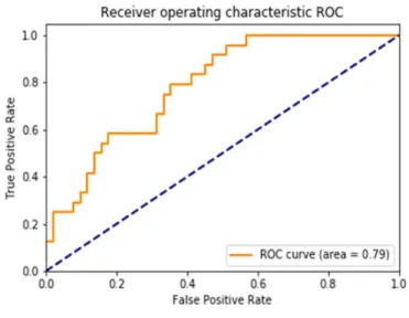
2.5.5 Area under the ROC curve ... 40
2.5.6 Kappa ... 41
2.6 Resampling techniques ... 42
2.6.1 Cross-validation method/leave one out validation ... 42
2.6.3 Holdout and random subsampling ... 43
2.6.4 Bootstrap method ... 44
2.6.5 Boosting and AdaBoost ... 44
2.6.6 Bagging ... 44
2.7 Model tuning ... 45
2.8 Conclusion ... 45
Methodology ... 47
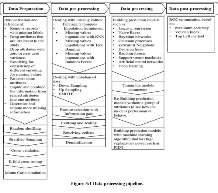
3.1 Data processing pipeline... 47
3.2 Statistical and machine learning models ... 48
3.3 Linear regression ... 50
3.4 Penalised models... 52
3.5 Logistic regression... 53
3.6 Naive Bayes ... 54
3.7 Bayesian networks ... 55
3.8 Linear and quadratic discriminant analysis ... 56
3.9 Gaussian processes ... 58
3.10 k-Nearest Neighbour ... 59
K-Nearest Neighbour rule ... 59
3.11 Decision trees ... 60
Decision tree learning algorithms ... 63
3.11.1C4.5 algorithm ... 65
3.11.2 CART, CHAID, and QUEST algorithms ... 67
3.11.3Random forests ... 67
3.12 Support vector machines ... 69
3.12.1Linear SVM ... 71
3.12.2Polynomial SVM ... 71
3.12.3 Radial SVM ... 71
3.13 Artificial neural networks ... 72
3.13.1Deep learning ... 74
3.14 Conclusion ... 75
Novel prediction modelling and pattern detection approaches for the first-episode psychosis associated with cannabis use ... 76
4.1 Problem description ... 77
4.2 Predicting first-episode psychosis: a computationally intensive approach ... 79
4.2.1 Data pre-processing ... 80
4.2.2 Training and optimising predictive models ... 84
4.2.3 Monte Carlo simulations ... 86
4.3.1 Predicting first-episode psychosis without cannabis attributes ... 89
4.3.2 Cannabis use and first-episode psychosis associations ... 90
4.3.3 Cannabis use duration and first-episode psychosis associations ... 92
4.4 Conclusion ... 93
A new machine learning framework for understanding the link between cannabis use and first-episode psychosis ... 94
5.1 Problem description ... 95
5.2 Methods ... 95
5.2.1 Data pre-processing ... 95
5.2.2 Predictive modelling ... 97
5.2.3 Predictive model post-processing ... 97
5.2.4 Overall modelling procedure ... 98
5.3 Results ... 99
5.4 Conclusion ...102
Predicting first-episode psychosis associated with cannabis use with artificial neural networks and deep learning ...104
6.1 Problem description ...105
6.2 Methods ...106
6.2.1 A trade-off between the extent of missing values and the dataset size ...106
6.2.2 Missing values imputation ...108
6.2.3 Training and optimising (tuning) predictive models ...108
6.2.4 Treating unbalanced classes ...109
6.2.5 Increasing model performance via optimised cut-off point selection on the ROC curve ...111
6.2.6 Monte Carlo simulations with neural networks and deep learning ...112
6.3 Results and discussion ...113
6.3.1 Attributes’ predictive power with respect to neural networks models and the t-test, and with the ROC approach ...115
6.4 Conclusion ...116
PIDT: A novel decision tree algorithm based on parameterised impurities and statistical pruning approaches ...118
7.1 Problem description ...119
7.2 Impurity measures ...121
7.2.1 Mathematical formulations ...121
7.2.2 Parameterised impurity measures ...123
7.3 S-pruning ...126
7.3.1 S-condition ...126
7.4.1 Predicting first-episode psychosis with the PIDT algorithm ...128
7.4.2 Additional experimental analysis ...130
7.5 Conclusion ...133
Conclusion and directions for future work ...135
8.1 Conclusion ...135
8.2 Future work ...136
REFERENCES ...138
Appendix 1 ...148
L
IST OF
F
IGURES
Figure 2:1 Generated datasets. ... 23
Figure 2:2 Box plot for a single attribute. ... 29
Figure 2:3 The ROC curve. ... 41
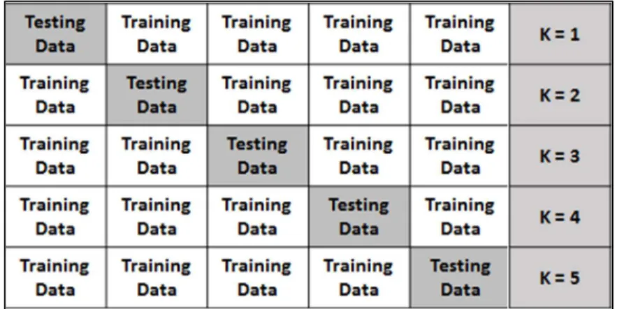
Figure 2:4 Five-fold cross-validation. ... 43
Figure 3:1 Data processing pipeline. ... 48
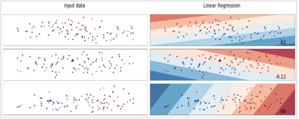
Figure 3:2 Linear regression. ... 51
Figure 3:3 Linear regression on generated datasets. ... 52
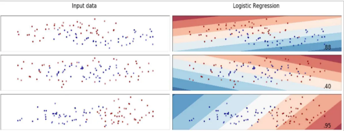
Figure 3:4 Logistic regression on generated datasets. ... 54
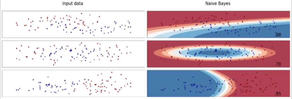
Figure 3:5 Naive Bayes on generated datasets. ... 55
Figure 3:6 Bayesian network ... 55
Figure 3:7 LDA and QDA on generated datasets ... 57
Figure 3:8 Gaussian Process classifier... 58
Figure 3:9 K-Nearest Neighbour ... 59
Figure 3:10 K-Nearest Neighbour on generated datasets ... 60
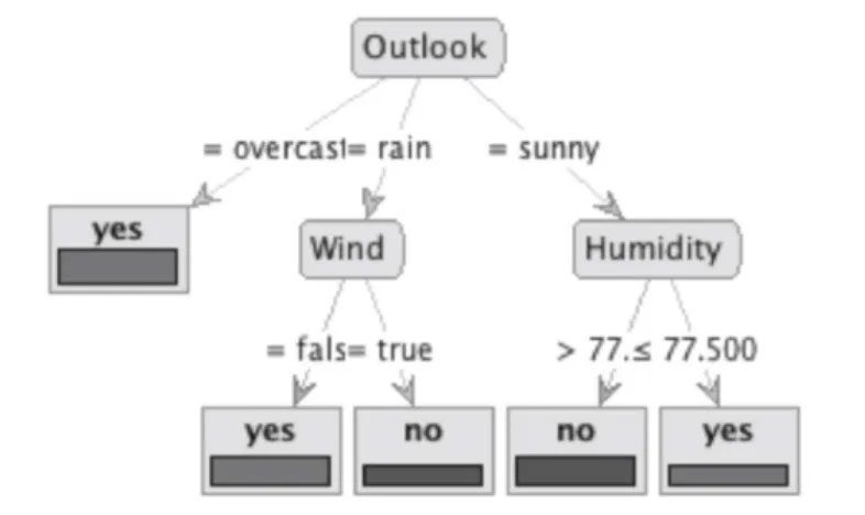
Figure 3:11 Decision tree for the weather problem ... 63
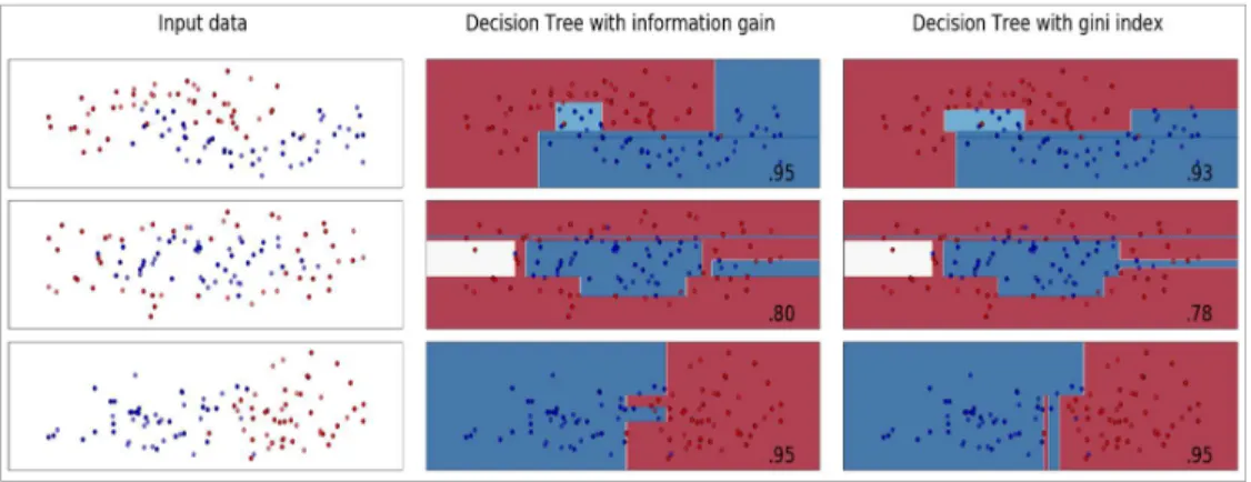
Figure 3:12 Decision tree classifiers on generated datasets ... 66
Figure 3:13 Basic random forests. ... 68
Figure 3:14 Random forest and AdaBoost on generated datasets ... 69
Figure 3:15 A linear Support Vector Machine. ... 71
Figure 3:16 Support Vector Machine with a radial kernel. ... 72
Figure 3:17 Support Vector Machines on several generated datasets. ... 72
Figure 3:18 Typical architecture of Artificial Neural Networks. ... 73
Figure 3:19 Neural networks on generated datasets. ... 74
Figure 4:1 Summary of the ratio of missing values for each attribute ... 83
Figure 4:2 Summary of the implemented methodology ... 87
Figure 4:3 Monte Carlo simulations. ... 88
Figure 4:4 Top association rules. ... 90
Figure 4:5 Bayesian Network for cannabis variables. ... 91
Figure 4:6 Histogram of the cannabis use duration attribute... 93
Figure 5:1 Attributes’ predictive power with respect to Information Gain. ... 96
Figure 5:2 ROC curves for 3 models: SVMR, GPP and GPR. ... 98
Figure 5:3 Summary of the implemented methodology with the k-fold cross-testing method. ... 99
Figure 5:4 2000 repeated experiments simulations on Support Vector Machines with Radial (SVMR) and Polynomial kernels (SVMP) and Gaussian Processes with Radial (GPR) and Polynomial kernels (GPR). ... 100
Figure 5:5 Left: ROC curves for optimised SVMR, with and without the cannabis attributes. Right: boxplots for 2000 repeated experiments simulations for optimised SVMR, with and without the
cannabis attributes... 102
Figure 6:1 Model performance for record and attribute cutting points. ... 107
Figure 6:2 Left: ROC curves for 2 of our optimised neural network (NN) models: single-layer NN and multi-layer NN. Right: ROC optimisation post-processing of the multi-layer NN model, with 3 optimal cutting points: maximum accuracy, Youden and top-left methods. ... 112
Figure 6:3 Summary of the implemented methodology with the k-fold cross-testing method and, a trade-off between the extent of missing values and the dataset size. ... 113
Figure 6:4 2000 Monte Carlo simulation for neural networks. ... 114
Figure 6:5 2000 Monte Carlo simulation for deep networks. ... 114
Figure 7:1 Parameterised entropy (PE) with different values for α. ... 123
Figure 7:2 Novel parameterised impurity measures PE, PG (top), and GE (bottom). ... 126
Figure 7:3 Unpruned decision tree for Pima diabetes ... 132
Figure 7:4 Pruned decision tree for Pima diabetes ... 132
Figure 7:5 Unpruned decision tree for glass dataset ... 133
L
IST OF
T
ABLES
Table 2:1 The Confusion Matrix and the evaluation measures: true positive TP, true negative TN,
false positive FP, false negative FN, positive P, and negative samples N. ... 39
Table 3:1 Probability distribution table for cannabis type ... 56
Table 3:2 Probability distribution table for cannabis frequency ... 56
Table 4:1 Cannabis use attributes in the analysed dataset ... 82
Table 4:2 Summary of parameters tuned for each model. ... 85
Table 4:3 Initial estimation of model accuracy. ... 85
Table 4:4 Initial estimation of model kappa. ... 86
Table 5:1 Estimations of the predictive models’ performances. ... 101
Table 6:1 Estimations of the predictive models’ performances. ... 114
Table 6:2 ROC curve attribute importance. ... 116
Table 7:1 Assessing decision trees built with conventional impurity performances. ... 131
Table 7:2 Assessing decision trees built with the PIDT algorithm with parameter optimisation, and with and without S-pruning procedure activated. “-” mean values do not apply. ... 132
Introduction
1.1
Research context and motivation
From the day life existed, decision making has been a part of the evolution of the human species. Humans make most of their decisions based on information and their ences. To make an accurate decision they usually look for patterns in their past experi-ments, and then decide on their best action. At present, more data and experiences have become available due to the massive increase in computers' abilities.
In many domains, where data is growing rapidly, there is always useful hidden information that needs to be extracted. For example, current patient records are stored on a regular basis, and this data may be used in extracting patterns for diseases, or for esti-mating health risk automatically, etc. Therefore, there is a need for knowledge discovery methods to be devised and applied to such data [1].
The process of deriving knowledge from data has long existed, and was previ-ously based on traditional statistical analyses and interpretations. These analyses and in-terpretations for data domains such as health, finance, business, and marketing usually rely on the specialists' skills to read into the data, which makes these analyses and inter-pretations costly and often only able to produce limited results. As adequate computer capacity and the volume of data increase, traditional approaches are often inappropriate. In this context, modern machine learning techniques are suited to improve the quality of these analyses and interpretations significantly.
The field of machine learning has advanced at a tremendous pace in recent years, with advanced predictive techniques being developed and improved upon. In order for these technologies to become truly refined, they must be applied to a variety of fields and subsequently challenged to find relevant solutions [2]. One such area of application is the field of medical research, which has a broad range of potential uses for machine learning [3] [4] [5].
Recently, machine learning techniques have emerged as a promising approach to medical prediction. For instance, recent works have sought to compare a variety of algorithms in predicting patient survival after breast cancer [6] and surgery for hypo-cellularity carcinoma [7]. In addition, machine learning techniques have proven their
abil-ity in predicting mental diseases such as Alzheimer’s [8]. These studies suggest that ma-chine learning can provide medical research with powerful techniques beyond the tradi-tional statistical approaches mostly used in this area, such as statistical tests, linear, and logistic regression. In biomedical engineering, several recent papers have explored the potential for classification algorithms to detect disease [9] [10]. This has led to the publication of additional guidance for medical researchers on how to interpret and question such findings [11]. Last but not least, there is tremendous interest in current interdisciplinary research into exploiting the power of machine and statistical learning to enable further progress in the new and promising area of precision medicine, in which predictive modelling plays a key role in forecasting treatment outcomes, and thus decisively contributes to optimising and personalising treatments for patients [5] [12].
A promising new approach is the use of computational modelling approaches to psychiatry [4]. Computational psychiatry has made it possible to combine enormous lev-els and types of computation with several types of data in an effort to advance classifica-tion of mental disease, predict treatment outcomes, and improve treatment selecclassifica-tion [13] [14].
Computational psychiatry is considered an essential area of research, yet there are still many difficult tasks that need to be carried out precisely and efficiently. Most studies in medical research (such as psychiatry) are only explanatory research and do not involve risk prediction modelling using machine learning algorithms. Moreover, incom-plete or inconsistent records, as well as the methodologies used (based mostly on conven-tional and straightforward statistical methods as pointed out above) limit many existing studies. These methods are traditionally well recognised and used in medical research (such as psychiatry), but in many situations do not match the great potential of modern machine learning methods.
Motivated by the above discussion, the present work is devoted to proposing synergistic statistical and machine learning approaches to medical data mining and pre-cision medicine in the area of psychiatric research. In particular, this dissertation proposes a predictive modelling approach to data-driven computational psychiatry.
1.2
Thesis statement
This document advances research in data mining via two phases. In the first phase, this dissertation focuses on developing a synergistic statistical and machine learning approach to medical data mining and precision medicine to improve patient care. In particular, this work proposes novel prediction modelling and pattern detection approaches for the first-episode psychosis associated with cannabis use. A significant effort in this study was the data pre-processing due to inherent challenges present in data collected in a case-control study involving many missing values, multiple encodings of related information, and a significantly large number of variables, etc. The innovative approaches are built upon several machine learning techniques whose predictive models have been optimised in a computationally intensive framework. Then, a new computationally intensive machine learning framework for understanding the link between cannabis use and first-episode psychosis was introduced. Finally, prediction models for the first-episode psychosis as-sociated with cannabis use were developed using artificial neural networks and deep learning with the proposed novel computationally intensive framework.
In the second phase, the dissertation focuses on developing new machine learn-ing algorithms that are particularly suitable for medical research. In particular, we propose novel and enhanced algorithms that produce models with high explanatory power, such as decision trees based on new families of impurities and statistical pruning approaches. The novel decision tree algorithm called PIDT, which is based on parameterised impuri-ties and statistical pruning approaches, is proposed and tested with several medical da-tasets.
1.3
Aims and objectives
The aim of this thesis is to develop predictive modelling data-driven approaches to com-putational psychiatry to advance classification of mental disease, predict treatment out-comes, or improve treatment selection. To this end, the thesis proposes synergistic statis-tical and machine learning approaches to medical data mining and precision medicine in the area of psychiatric research. It also proposes new machine learning algorithms that have high explanatory power and are particularly suitable for medical research.
To this end, several medical datasets are presented to report the advantages and the disadvantages of the machine and statistical learning algorithms. This includes the clinical psychiatry data (first-episode psychosis - cannabis clinical dataset) introduced to build novel predictions models and to detect new patterns in patients’ data [15]. The clinical psychiatry data was used to develop predictive modelling data-driven approach to computational psychiatry to advance classifications of mental disease. In order to accomplish this aim, the following objectives should be met.
Objective 1: systematically review and analyse the area of computational psychiatry and the challenges involved.
Objective 2: Derive statistical and machine learning methods for predictive modelling of mental diseases, focusing on psychosis associated with cannabis use, and investigate their use and performance.
Objective 3: Propose approaches to further enhance the predictive value of the derived methods.
Objective 4: Derive methods with high explanatory power suitable for computational psychiatry research.
The above objectives are associated with some important research questions that the thesis aims to answer.
I. Can one use a clinical data to build prediction models for mental diseases such as the first-episode psychosis associated with cannabis use? This refers to Objective 2. II. How can one improve the prediction of mental illness in the presence of a
signifi-cantly large number of missing values and unbalanced classes in case-control data? What is the variability of predictions in the presence of missing values? Are these prediction models stable enough? These refer to Objective 3.
III. Do some predictors, such as cannabis use attributes, in clinical psychiatry data [15] have predictive information for mental illness, such as the first episode psychosis? What is the predictive value of these predictors on mental illness, such as first epi-sode psychosis? These refer to Objective 2 and 3.
IV. Can the prediction models be improved with post-processing techniques? Can the prediction models be improved via optimising the cut-off point selection on the ROC curve? These refer to Objective 3.
V. Can one develop a new machine learning algorithm that has high explanatory power, such as decision trees, for medical research? This refers to Objective 4.
VI. How attribute selection should be done and what impurity measures should be used? How overfitting can be avoided? These refer to Objective 4.
1.4
Methodology
Different research problems involve different research methodologies. The main categories of research approaches that were used in the thesis are experimental research, build research, process research and simulation research. These research strategies are described as follow. The first methodology, which is mainly used, is the experimental methodology which uses experiments designed to test hypothesis. It often involves record keeping, experimental setup design, and experimental results reporting. All the experiments and results should be reproducible. The second methodology is the build methodology which often encompasses designing the software system, reusing components, choosing an adequate programming language, and considering testing all the time. The third methodology is the process methodology which often includes soft-ware process, methodological issues, and cognitive modelling. The final methodology is the simulation methodology which uses computer simulations to address question difficult to answer in the real application.
This thesis includes several comparative studies which usually employ several techniques, and try to find which one is better. Answering this question should be for a given purpose, which is not necessarily absolute ranking, such as proposing predictive modelling approaches to data-driven computational psychiatry. Other research questions like “where are the differences?” and “What are the trade-offs?” need to be answered as well in this research method.
The above research method should be applied to a “clinical psychiatry data” and typically compared in the form of a table.
1.5
Structure of the thesis and contributions
The thesis is organised as follows. Background information on the machine learning mod-elling procedure was used to establish the results in this work, and strategies to improve
the procedures are provided in Chapter 2. The overall data processing frame-work/pipeline is proposed in Chapter 3 as well as a series of standard results, defi-nitions, and models of existing statistical and machine learning algorithms related to this study are reviewed. In Chapter 4, novel prediction modelling and pattern detection ap-proaches for first-episode psychosis associated with cannabis use are derived. A new machine learning framework for understanding the link between cannabis use and episode psychosis is presented in Chapter 5. More powerful prediction models for first-episode psychosis associated with cannabis use via neural networks and deep learning, are provided in Chapter 6. A novel decision tree algorithm PIDT based on new families of impurity measures and statistical pruning approaches for building optimised decision trees are introduced and used to understand successfully the link between cannabis use and first-episode psychosis in Chapter 7. In Chapter 8, conclusions are drawn, and future research directions are discussed.
Overall, the thesis is organised into six chapters and a common conclusion. The main contents of each chapter are briefly outlined below.
Chapter 2 – Background and problem. Background information on the machine learn-ing modelllearn-ing procedure is used to establish the results in this work, and strategies to improve them are set out in this chapter. This includes information on the data used in this dissertation, data preparation techniques, resampling techniques, and estimating the model performances.
Chapter 3 – Methodology. This chapter presents the general data processing frame-work/pipeline first, and then it will allow customising/tailoring this framework to fit the needs of each chapter. The proposed framework can be tailored to the needs of a particular dataset, or to answer a specific research question, by using a particular method/technique. Also, a series of standard results, definitions, and models of the existing statistical and machine learning algorithms related to this study are provided.
Chapter 4 - Novel prediction modelling and pattern detection approaches for the first-episode psychosis associated with cannabis use. The predictive value of cannabis-related variables concerning first-episode psychosis is demonstrated in this chapter by showing that there is a statistically significant difference between the performance of the
predictive models built with and without cannabis variables. We were inspired in this approach by the Granger causality techniques [16], which are used to demonstrate that some variables have predictive information on other variables in a regression context, as opposed to classification, which is mainly the case in our framework. Moreover, we in-vestigate how different patterns of cannabis use relate to new cases of psychosis, via association analysis and Bayesian techniques such as Apriori and Bayesian Networks, respectively.
Chapter 5 - A new machine learning framework for understanding the link between cannabis use and first-episode psychosis. This chapter proposes a refined machine learning framework for understanding the links between cannabis use and first episode psychosis. The novel framework concerns extracting predictive patterns from clinical data using optimised and post-processed models based on Gaussian processes and support vector machines algorithms. The cannabis use attributes’ predictive power is investigated and we demonstrate statistically and with ROC analysis that their presence in the dataset enhances the prediction performance of the models with respect to models built on data without these specific attributes.
Chapter 6 – Predicting first-episode psychosis associated with cannabis use with ar-tificial neural networks and deep learning. This chapter proposes a novel machine learning approach, based on neural networks and deep learning algorithms, to developing highly accurate predictive models for the onset of first-episode psychosis. Our approach is also based on a novel methodology of optimising and post-processing the predictive models in a computationally intensive framework. A study of the trade-off between the volume of the data and the extent of uncertainty due to missing values, both of which influence predictive performance, enhanced this approach. The performance capabilities of the predictive models are enhanced and evaluated by a methodology consisting of novel model optimisation and testing, which integrates a phase of model tuning, a phase of model post-processing with ROC optimisation based on maximum accuracy, Youden and top-left methods, and a model evaluation with the k-fold cross-testing novel methodology (explained in the previous chapter). We further extended our framework by investigating cannabis use attributes’ predictive power and demonstrating statistically that their presence in the dataset enhances the prediction performance of the artificial
neural networks presented in this chapter. Finally, the model stability is explored via simulations with 2000 repetitions of the model building and evaluation experiments. Chapter 7 - PIDT: A novel decision tree algorithm based on parameterised impuri-ties and statistical pruning approaches. This chapter presents novel splitting attribute selection criteria based on some families of parameterised impurities that we propose here to be used in the construction of optimal decision trees. These criteria rely on families of strict concave functions that define the new generalised parameterised impurity measures that we applied in devising and implementing our PIDT novel decision tree algorithm. This chapter also proposes the S-condition based on statistical permutation tests, whose purpose is to ensure that the reduction in impurity, or gain, for the selected attribute is statistically significant. The idea behind proposing such algorithms is to build accurate prediction models that are easy to interpret and explain to psychiatry experts.
Chapter 8 - Conclusion and directions for future work. The main results are summarised, and future research directions are discussed.
Background and problem
definition
2.1
Data-driven computational psychiatry
Machine learning algorithms have already begun to prove their particular capabilities in and contributions to medical research and applications [4]. In particular, machine learning techniques have been successfully used in diagnosing psychosis [17], analysing diabetic patients’ data [18] [19], classifying leukaemia [20], and detecting heart conditions in elec-trocardiogram (ECG) data [21], etc. These studies show that machine learning has proven to be capable of dealing with challenging medical data, in particular with the ambiguous nature of the ECG signal data, for which machine learning algorithms show outstanding results compared to other methods [20] [21].
These days, more health care providers are replacing traditional paper notes with electronic patient records. In addition, the use of advanced technologies, such as comput-ers, personal digital assistants, smartphones, etc., has enabled information to become more available and accurate [3]. This led to a tremendous increase in the electronic health data, creating a promising basis for applying machine learning algorithms to extract in-sights from data.
Currently, machine learning algorithms are in the process of revolutionising health. In the same way as machine learning has made an enormous difference to business and industry, it will just as undoubtedly enhance medical research and improve the prac-tice of healthcare providers. The medical field is considered a critical area of research, yet there are still many difficult tasks that need to be carried out precisely and efficiently. The future success of health sector planning, and of health care in general, will be in the adoption of intelligent systems where robotics and machine learning intersect. In order for health sector planning to catch up with this fast-changing environment, machine learn-ing must be at the core of most strategies. For example, new developments in psychiatry concern the so-called data-driven computational psychiatry, which relies heavily on the use of machine learning [4]. Data-driven computational psychiatry has made it possible to combine enormous levels and types of computation with several types of data in an
effort to advance classification of mental disease, predict treatment outcomes, or improve treatment selection [13] [14].
Most studies in medical research (such as psychiatry) so far are only explanatory research and do not comprise risk prediction modelling using machine learning algo-rithms. In addition, many existing studies are limited by incomplete or inconsistent rec-ords, but also by the methodologies used, which are based mostly on conventional and straightforward statistical methods. These methods are traditionally well recognised and used in medical research (such as psychiatry), but in many situations, they do not match the large potential of the modern machine learning methods.
In this chapter, we discuss and summarise different machine and statistical learn-ing techniques that are suitable for use in the medical field, especially in psychiatry. Med-ical research involves many problems that benefit from analysing data based on tech-niques of data pre-processing, predictive modelling, clustering, and so on. In predictive modelling in particular, the task is to predict the outcome associated with a particular patient given a feature vector describing that patient. In clustering, patients are grouped because they share similar characteristics, and in data pre-processing operations such as feature selection, the task is to select the most relevant attributes to predict the outcome for a patient [2].
Many of these data pre-processing algorithms are described in this chapter. How-ever, we should note that no single algorithm is superior to others in all the problems. The algorithm needs to match the structure and the particularities of the problem at hand, in order to obtain useful information or an accurate model. The ultimate aim is to develop models that use predictors or known features to create predictive models that will be utilised for predicting the output [22]. However, choosing the suitable algorithm and de-veloping a model are not the only aspects we need to consider; other data mining phases such as data pre-processing and model post-processing are also involved. Therefore, ex-tracting knowledge from data involves all these phases of processing.
The first stage, which is the pre-processing stage, has three sub-processes: data filtering, data cleaning, and data transformation and projection. Data filtering is respon-sible for the selection process of relevant data to be analysed. Data cleaning involves handling data problems such as treating missing values, smoothing noise in data, remov-ing outliers, etc. Data transformation is responsible for aggregation, normalisation, and
unit conversion, and helps to speed up the process, improve performance, and decrease problem complexity.
The processing stage consists of some sub-processes such as model generation, tuning and building, and evaluating the output model. Model generation and tuning are some of the most critical sub-processes. The model generation and tuning are iterative processes comprising three steps: choosing the algorithm and its parameters, building the model, and evaluating the model. The goal of this process is to find the best parameter values for the model and thus assess the performance of an algorithm for the problem at hand [23].
The last stage is the post-processing stage, which is responsible for knowledge presentation and improving the model performance. Knowledge presentation is used to display the extracted knowledge comprehensively. Finally, based on the results from the entire data mining process, the best performing model is applied to the current problem.
The essential question when dealing with machine learning is not whether a learning algorithm is favoured over others, but under which conditions a certain devel-oped prediction model can significantly outperform others for a given application prob-lem. This chapter provides a literature review of several strategies to improve these sta-tistical and machine learning prediction algorithms. Moreover, the several datasets used in this work are outlined in this chapter. Synthetically generated datasets are used to report the advantages and the disadvantages of several machine and statistical learning algo-rithms. In addition, clinical data was used to build novel predictions models and detect new patterns in the data.
The above techniques are used in the remainder of the thesis to propose novel synergistic machine learning and statistical approaches to pattern detection and to develop predictive models for research questions such as predicting first episode psychosis.
2.2
Sources of datasets
Several datasets were used throughout the document. Randomly generated datasets were used in the literature to report the advantages and the disadvantages of several machine and statistical learning algorithms on various types of datasets. Other datasets such as clinical data were used to build novel prediction models and to detect new patterns in that
particular dataset. Finally, some public data was used to validate the decision tree classi-fiers produced with the novel PIDT algorithm that we propose in chapter 7. The selected datasets can be grouped into synthetically generated datasets, clinical datasets, and public datasets.
2.2.1
Generated datasets
Three synthetic datasets were generated to illustrate the nature of decision boundaries of different classifiers and to give an overview of how different classifiers perform on vari-ous synthetic datasets using a package called scikit-learn 0.19.1 (October 2017) [24]. Each of the three datasets has 100 samples. Each sample has two input attributes and one output attribute that represents the class membership of each sample. The three generated datasets are:
Moons dataset, which contains samples in the form of two interleaving half-circles.
Circles dataset, which contains samples in the form of a larger circle containing a smaller circle.
Linear dataset, which contains samples that are linearly separable.
Moons Dataset Circles Dataset Linear Dataset
Figure 2:1 Generated datasets.
Each of these three datasets has some noise added in order to simulate real situ-ations in which data and classificsitu-ations are not perfect. Figure 2:1 presents the data points for the three generated data sets. The plots show training points in solid colours and test-ing points in semi-transparent colours.
2.2.2
First-episode psychosis - cannabis clinical dataset
This clinical dataset is a part of a case-control study at the inpatient units of the South London and Maudsley (SLaM) NHS Foundation Trust [15]. The dataset is also used in training and optimising the predictive models for first-episode psychosis in chapters 4, 5, 6, and 7. The clinical data consists of 1106 records, including patients and controls. Those described as patients were patients of the trust who at one time presented with first-episode psychosis; controls were recruited from the local area through the internet, news-paper advertising, and by distributing leaflets. Each record refers to a participant of the study and has 255 possible attributes, which were divided into four categories. The first category consists of demographic attributes that represent general features such as gender, race, and level of education. Secondly, drug-related attributes contain information on the use of non-cannabis drugs such as tobacco, stimulants, and alcohol. The third category is formed by genetic attributes. The final category contains cannabis-related attributes such as the duration of use, initial date of use, frequency, and cannabis type, etc. (See Appendix 2).
2.2.3
Public datasets
Five public datasets are used in chapter 7 to illustrate the performance of different impu-rity measures as splitting criteria for the decision trees built with our newly proposed PIDT algorithm. These datasets are as follows:
1. Breast Cancer Wisconsin (original) dataset from the UCI Machine Learning Repository [25]. This dataset comprises 569 observations and 30 numeric at-tributes. Each observation is in one of the two classes, malignant or benign. 2. Pima Indians Diabetes dataset from the UCI Machine Learning Repository
[25]. Ten measures (variables) were obtained for each of n = 442 diabetes patients over one year. The goal is a quantitative measure of disease progres-sion after one year.
3. Hepatitis dataset from the UCI Machine Learning Repository [25]. The hepa-titis dataset contains 155 examples of hepahepa-titis patients, described by 19 nu-meric and nominal attributes. Of these cases, 123 correspond to the patients who survived treatment (‘live’) and 32 examples of mortalities (‘die’).
4. The Primary Tumour dataset from the University Medical Centre, Institute of Oncology, Ljubljana, Yugoslavia [25]. The primary tumour dataset has 21 concepts and 17 attributes, and 207 out of 339 examples contain at least one missing value.
5. The glass identification dataset from the UCI Machine Learning Repository [25] comprises data representing a study of classification of types of glass, motivated by criminological investigations. At the scene of the crime, the glass left can be used as evidence, if correctly identified. This dataset contains 10 attributes regarding several glass types (multi-class).
2.3
Data preparation
Data preparation techniques refer to the process of adding, deleting, or transforming data. Data preparation can influence improving a model’s predictive ability. The choice of the predictive modelling techniques determines which strategies to apply. Some models, such as tree-based models, have the capacity to deal with numeric and nominal attributes. Oth-ers, like support vector machines, do not. In addition, some models, such as distance-based models, like k-nearest neighbour (k-NN), are very insensitive to the characteristics of the predictor data. Others, like linear regression, are not.
Prior to applying any statistical and machine learning algorithms, significant work effort is usually involved in the data pre-processing in order to deal with the chal-lenges present in the data sets. This section reviews several approaches to overcome these challenges in the data.
2.3.1
Dealing with missing values
In real-life data sets, the most common problem is incomplete data. Many applications have missing data for a variety of reasons. Sometimes the data collection was done im-properly. In some cases, participants interrupted their participation in a study. In other cases, the value for an attribute is unavailable. All these situations generate missing val-ues. A limited number of machine learning algorithms, such as C4.5 decision trees or Naive Bayes, can handle internally missing values, but the vast majority require prelimi-nary treatment of the missing values. Several methods exist for handling missing data. Some methodologies remove attributes or records that have a high percentage of missing
values [26]. Other methodologies treat the missing values by imputing them. This section presents techniques to deal with missing data, such as embedded methods for missing data, filtering missing data, and imputing missing data.
Decision tree prediction approaches have robust methods for handling incom-plete data, such as C4.5 [27]. In the training stage, the impurity of each attribute is adjusted by a factor depending on the number of available values in the training set for the same attribute. The classification and regression trees algorithm (CART) employs the surrogate variables splitting (SVS) technique. This method is for use during the prediction phase only [26]. The recursive partitioning and regressing trees (RPART) approach contains an extension of the previous methods to handle missing data during the training stage [28].
Filtering techniques remove incomplete data parts. The list-wise deletion method removes all incomplete instances so that it is suitable for the prediction models to use the remaining complete instances [29]. These methods may be practicable when the number of missing values is quite small compared with the remaining data set. There are two ways to filter and discard data with missing values. The first way is to keep complete instances only. The second method consists of determining the percentage of missing data on each record and attribute and deleting the record and/or attributes with missing data percent-ages below the specified threshold. Unfortunately, essential attributes could be discarded during this process. Therefore, extra care should be taken before removing any attribute. Imputation techniques assume that there is a relation between the attributes, so the objective is to apply prediction models to infer the missing values in one attribute using the existing values of other attributes in the dataset. This process is repeated until it produces a complete data set. Imputation replaces the missing data in a deterministic or stochastic way [1]. In the deterministic case, the missing value is replaced by a uniquely inferred value. In the stochastic case, the missing value is replaced by a random value from some distribution. Imputation methods may be global or local, depending on the volume of data.
On the one hand, global imputation techniques are of two main kinds: missing attribute and non-missing attribute methods. In the missing attribute method, new values are calculated for the missing data items based on analysing the existing values for the
attributes, by using mean, median, or mode. Although this technique has some bias to-wards a standard deviation, if we use a non-deterministic mean imputation method, we will get better performance because it produces random disturbance to the average. The main drawbacks of this approach are the potential generation of inconsistent data and the complexity of the computation. In the non-missing attribute methodologies, we assume that there is a correlation between missing and non-missing values. These methodologies use the correlation to predict the missing data. Imputation by regression treats the missing data as a target attribute, and it performs regression to input missing values [30]. How-ever, this method also has some disadvantages. When selecting a suitable regression model, for example, only one value is derived for each missing data, which fails to rep-resent the uncertainty associated with missing values. In 1987, Rubin proposed a new technique of imputation to overcome the uncertainty problem in linear regression. Multi-ple imputations consist of three stages: produce m-comMulti-plete data sets through single iputation, analysis of each of the data sets, and the combination of the results of the m-analyses into the result [31].
On the other hand, there are many techniques for local imputations. Local impu-tation methods do not have a theoretical formulation but have been implemented in prac-tice [32] [33] [34]; the imputation uses a supervised learning technique such as K-NN and bagging trees. The k-NN imputation uses the k-NN algorithm to estimate and substitute missing data. It tries to find similar records for the current record and to impute the miss-ing value from the correspondmiss-ing values of the neighbourmiss-ing records. The main benefit of this approach is that it can predict both discrete attributes and continuous attributes. It uses the most common value for discrete attributes and the mean value for numeric at-tributes. Other algorithms, such as bagging trees, have also confirmed their ability in many applications in practice [35]. In the bagging tree imputation, the algorithm treats the attribute that contains missing values as an output attribute, and it builds the tree using the remaining attributes. Then, the algorithm imputes the missing values in the output attribute using the built tree. The imputation iterates through the attributes until there are no missing values.
2.3.2
Centring and scaling
In both statistics and machine learning, centring and scaling numeric attributes are often crucial prior to building prediction models, in order for a particular model to perform accurately. Centring and scaling are regularly adapted to support the numerical stability of the computations during building prediction models. For instance, the K-NN algorithm requires the attributes to have a standard scale to be developed accurately, since it depends directly on measuring the distance between records. In addition, these manipulations are needed when regression models are being generated because if the predictors have several units and ranges, the final model will have disproportionate coefficients, which makes it difficult to interpret. Moreover, centring and scaling could be employed first when build-ing penalised models such as lasso regression and ridge regression, since the penalty in these methods is calculated based on the estimated coefficients.
To centre an attribute, the mean value of that attribute is subtracted from all val-ues of the attribute. As a result of this process, the attribute will have a mean value that is equal to zero. Then, to scale the attribute, the values of the attribute are divided by the calculated standard deviation. As a result of this process, the attribute will have a standard deviation equal to one. To centre and scale an attribute 𝑥 the following equation is em-ployed on each data point 𝑟, 𝑤here 𝑟 ranges from 1 to 𝑛.
𝑥∗ =𝑥 − 𝑥̅
𝜎
Above 𝑥∗ is the new value of the predictor c for the 𝑟 data point, 𝑥̅ is the mean
of the 𝑛 values of the predictor 𝑐, and 𝜎 is the standard deviation of the 𝑛 values of the predictor 𝑐. The only disadvantage of these transformations is the loss of the real values of the individual records since the data are no longer available in the original range or units.
2.3.3
Resolving outliers
Outliers are samples that are abnormally far from the mainstream of the data. In both statistics and machine learning, dealing with these outliers is necessary before building accurate prediction models. Outliers can mislead the training process resulting in prolonged training times and less accurate models. Some predictive models, such as
tree-based prediction models and SVM, are resistant to outliers. However, other models such as logistic regression and neural networks are not.
One way to deal with the outliers is to detect them and then to delete them. Out-liers can be recognised easily by looking at some plots such as the box plot. A single box plot for one attribute is shown in Figure 2:2, where the plot shows the median, the first and the third quartile, and the outliers. When some samples are suspected to be outliers, these samples should be removed from the dataset, especially if the used prediction model is considered sensitive to outliers. However extra care should be taken when removing samples, especially if the dataset size is small, otherwise sensitive data may be wasted.
Figure 2:2 Box plot for a single attribute.
Another way to deal with the outliers is to transfer the attributes using the spatial sign [36]. The spatial sign projects the attribute values into a multidimensional sphere. This process will have the effect of making all the samples have the same distance from the centre of the sphere. Mathematically, each sample is divided by its squared norm, and the equation is as follows:
𝑥∗ = 𝑥
∑ 𝑥
Where 𝑥∗ is the new value of the 𝑐 predictor for 𝑟 data point, where 𝑟 range from 1 𝑡𝑜 𝑛 and where 𝑐 ranges from 1 𝑡𝑜 𝑚 . This approach is intended to measure the distances between the attributes. Therefore, it is important to centre and scale the attribute applying the above approach.
2.4
Feature selection
Feature selection methods are recommended when the predictor's number is too large compared to the sample size, resulting in the model scoring high accuracy on the training data but performing very poorly on the test data [37]. In the feature selection process, we select specific predictors to avoid the problem of over-fitting [38]. Mostly, the feature selection reduces the dimension of data, which also speeds up the data mining process, decreases computational cost, and overcomes over-fitting. However, reducing some at-tributes may cause loss of information and might lead to worse results. In 2007, Nilsson mentioned the two main categories of feature selection problems, which are finding the optimal predictive attributes for building efficient prediction models and finding all the relevant attributes for the class attribute [39].Feature selection algorithms have some fundamental processes that affect the nature of the search for the best attributes, such as the starting point, the search organisa-tion, the evaluation strategy, and the stopping criterion [40].
The point of departure is choosing a point in the predictors subset to begin the search. The selection point may be taken with no predictors, with all predictors, or some-where in the middle. If the selection point is selected with no predictors, this methodology will start by adding predictors and proceeding forward through the search space. If the selection point is chosen with all predictors, it will start removing the predictors and pro-ceed backwards through the search space. Finally, if the selection point is in the middle, the methodology will start adding predictors and proceed outwards from that point.
Secondly, the search organisation is the search strategy that may be an exhaus-tive search or a heuristic search. In the exhausexhaus-tive search, the methodology starts with a small number of predictors. With x initial predictors there exist 2X possible subsets. Alt-hough a heuristic search is more feasible than an exhaustive search and gives good results, it cannot guarantee to find the optimal attribute subset.
Thirdly, the evaluation process is the primary factor that differentiates between different feature-selection algorithms. The evaluation process is done by filters or wrapper techniques. Filters are used to remove the undesirable predictors of the data be-fore learning begins. Wrapper techniques use a combination of induction algorithms and statistical re-sampling techniques [41].
Fourthly, the stopping process has to be determined by the feature selector meth-ods. Feature selectors may stop adding or removing predictors depending on an evalua-tion strategy. If the alternative predictor does not improve upon the merit of a current predictor subset, it will stop. An alternative option is to continue generating predictor subsets until the opposite end of the search space and then choose the best subset.
There are two main categories of feature selection. The first type is to find the best subset of predictive features, which helps produce efficient prediction models. The second type is to find all the relevant predictors for the class attribute, which could be achieved by performing a ranking on the attributes according to their predictive powers. Predictive power measures are done by first computing the performance of the classifier built with every single variable, by computing statistic measures such as correlation co-efficient or by applying information theory measures such as the mutual information [37].
2.4.1
Search strategies
Search strategies apply a complete search for the best predictors subset according to the evaluation function used. Heuristic search procedures consist of efficient ways to provide solution quality and decrease the search complexity. Many techniques of search strategies in this category take into consideration the remaining predictors for selection/rejection for any iteration. Therefore, these techniques are relatively fast. Many search techniques could be used for the search strategies, such as greedy hill climbing, stepwise bi-direc-tional search, best-first search, and genetic algorithms. Genetic algorithms consider global changes and usually reach the optimal global solution. Greedy hill climbing search considers the local modification to the predictor's subset, and it can determine a locally optimal solution. Best-first search considers local modification and allows backtracking along the search path.
Greedy hill climbing is a simple search technique, which examines the local changes to the current predictor's subset. Local changes add or delete a single predictor from the subset. If the algorithm starts adding predictors, it will make a forward selection. However, if the algorithm will delete a feature, it will do a backwards elimination [42] [43]. Another option is the stepwise bi-directional search, which uses both adding and deleting predictors. In this technique, the search algorithm considers all possible local
changes to the current subset and selects the best one, or it may choose the first real im-provement. If one change is accepted, it will not reconsider once again.
Best first search is an artificial intelligence search technique [44]. It is similar to greedy hill climbing in allowing backtrack along the search path. In addition, the best first moves in the search space will be the current predictor set. However, this technique is not like the greedy hill climbing. When the search seems less promising, it will backtrack to the more promising subset. Furthermore, this technique will explore the entire search space and will use the stop process to limit the number of subsets that result in no im-provement.
Genetic algorithms are based on the idea of natural selection in biology [45]. Genetic algorithms and all evolutionary computation algorithms are an iterative process. The new generation is produced by applying genetic processes such as crossover, and mutation to the current generation. Mutation is done by changing the values in the subset randomly. However, the crossover is produced by combining two predictors from a pair of subsets into a new subset. The genetic processes are applied based on the value of their fitness, which is evaluated by evaluation techniques. After the assessment process, the better subsets will have a good chance to be used to create the new subsets through cross-over and mutation. The algorithm uses a population of solutions, which updates cross-over time to avoid trapping in a local minimum solution. In the feature selection process, the solu-tion is represented by the fixed binary string. The value of each posisolu-tion in the binary string represents the status of a particular feature that may be presence or absence.
2.4.2
Feature selection filters
The primary goal of feature selection is to get efficient attributes to build accurate predic-tion models. In addipredic-tion, feature selecpredic-tion could be used to minimise the probability of error (Bayesian). The filters employ feature selection regardless of the type of classifier but depend on the properties of the data distribution itself. There are many algorithms for the filtering process, such as RELIEF [46], Las Vegas Filter (LVF) [47], FOCUS [48], correlation-based filter (CFS) [49], and principal component analysis (PCA), as well as many statistical methods based on hypothesis tests.
In 1991, FOCUS was one of the earliest multivariate filters. The main drawback is that it cannot handle noisy data and it has a predisposition towards over-fitting [48]. In
1992, Kira proposed the RELIEF technique based on the nearest neighbour learner meth-odology [46]. The main drawback is that there is no methmeth-odology for choosing the neigh-bour sample size. In 1996, Liu used a probabilistically guided random search to explore the attribute subspace and proposed a method called LVF [47].
In 2010, Halalai et al. proposed a new filter to select those attributes that have a strong correlation with the target attribute and a weak correlation between each other [49]. Finally, PCA could be employed for feature selection. PCA has proven its ability in a large variety of applications including image processing and so on [50].
2.4.2.1
Consistency filters
In 1991, Almuallim and Dieterich proposed a new technique called FOCUS, which was designed for the Boolean domain [48]. FOCUS searches for predictor subsets until it finds the minimum combination of predictors that divide the training into the purist classes. The output will be a combination of predictor values in each class. The final predictor subset will be processed by an induction decision tree ID3 [51]. In 1994, Caruanna and Freitag claimed that there are two main difficulties with FOCUS [52]. Firstly, the FOCUS approach proposes to achieve consistency in the training data. However, the search pro-cess may become difficult because many of the predictors are needed to keep consistency. Secondly, this method produces a strong bias towards consistency, because the algorithm will continue to add predictors to fix a single inconsistency. In 1996, Liu and Setiono proposed a new algorithm similar to FOCUS, called Las Vegas Filter [47]. LVF works by generating a random subset S from the predictor subset during each round of execu-tion. The inconsistency rate described by S is compared to the inconsistency rate of the best subset. If the new subset S is consistent with the best subset, then S will be the new best subset. The inconsistency rate is calculated in two steps. Firstly, inconsistency count is the number of instances occurring in the group minus the number of instances occurring in the group with the most common class value. Secondly, the overall inconsistency is the sum of the inconsistency counts in all groups of a matching instance divided by the total number of instances. Liu and Setiono mentioned that due to the randomness of LVF, the longer it is allowed to execute the better the result. They tested the algorithm on two large datasets: the first has 65,000 instances described by 59 attributes, and the second has
5,909 instances described by 81 attributes. LVF achieved a good result and reduced the dataset by more than half in both cases.
2.4.2.2
Instance-based learning filter for feature selection
In 1992, Kira and Rendell proposed their new algorithm RELIEF, which uses instance-based learning to assign an appropriate weight to each predictor [46]. The weights of the predictors are used to distinguish between the class values. It uses the weights to reorder the predictors; the weights beyond the user-specified threshold are used to create the final subset. The algorithm randomly selects sample instances from the training data. Each instance will do two operations: nearest hit and nearest miss. In other words, it will find the closest instance in the same class (nearest hit) and the nearest instance in the counter class (nearest miss). The attribute's weight is updated according to the value of the in-stance in the closest hit and nearest miss as shown in the next equation:
𝑊 = 𝑊 − 𝑑𝑖𝑓𝑓(𝐶, 𝑅, 𝐻)
𝑚 −
𝑑𝑖𝑓𝑓(𝐶, 𝑅, 𝑀) 𝑚
As shown in the above equation, the weight of attribute C is updated, where R is a randomly sampled instance, H is the nearest hit, M is the nearest miss, and m is the number of randomly sampled instances. The difference function 𝑑𝑖𝑓𝑓 is a Boolean func-tion for nominal attributes, and it is used to test the existence of the difference between two instances for a given attribute; it assigns 1 if the values are different, or 0 if the values are the same. In the case of continues attributes, the diff function has a value between [0, 1. The output of all weights will be between the interval [-1, 1].
In 1994, Kononenko modified the RELIEF algorithm to work on multiple classes [53]. In 1997, Scherf and Brauer proposed a new instance-based technique called Euclid-ean Based Feature Selection (EUBAFES) [54]. EUBAFES is similar to RELIEF for de-termining separated clusters by reinforcing similarities between instances occurring in the same class while decreasing the similarity between instances of different classes.
2.4.2.3
Learning algorithm as a filter for another learning
algo-rithm
In these filter approaches, researchers used a particular learning algorithm as a filter to determine the best predictor subsets for a primary learning algorithm. In 1995, Cardie used the decision tree algorithm for the feature selection process [55]. K-NN classifier
has been used with the decision trees. This hybrid system achieved a better result than decision trees alone. In 1996, Singh and Provan used a greedy oblivious decision tree algorithm during the feature selection process to construct a Bayesian network [56]. The results showed that the Bayesian network combined with the oblivious decision tree al-gorithm outperformed the classical Bayesian network only.
In 1995, Holmes and Nevill-Manning used Holte's 1R system to calculate the predictive accuracy of individual predictors [57]. This technique is done without any searching; however, it depends on the user selecting the desired predictors from the ranked list. If we split the data into training data and testing data, the 1R method will be able to calculate a prediction accuracy for each rule and each feature on the training data. The predictors will be reordered due to prediction scores; the highest ranked predictors will be selected with any learning algorithm.
In 1995, Pfahringer used a program to get the decision table majority (DTM) classifiers to choose predictors [58]. DTM classifiers are a type of nearest neighbour clas-sifiers and are produced by greedy searching for search space. DTMs provide highly rec-ommended results when all predictors are nominal. Pfahringer used the concept of mini-mum description length (MDL) [59]. MDL was used to calculate the cost of encoding a decision table. Other learning algorithms use the predictors that are produced in the final determination table.
2.4.2.4
Principal component analysis
Principal component analysis (PCA) methodology exchanges the set of the original at-tribute with a new subset of uncorrelated atat-tributes that represent most of the data [60]. If an attribute misleads the prediction process, it is considered as being noise. A classifier would perform better if the noise in the data were removed. PCA can also be seen as one of the approaches for removing noise from the data. It assumes that directions in the data space along which data varies least are mostly due to noise. PCA is a way of detecting patterns in data by highlighting their similarities and differences between them.
Another advantage of principal component analysis is that once these patterns in the data are found, the data can be compressed, and the number of predictors can be reduced. An example of the use of the principal component analysis is seen in [50], where