HAL Id: hal-02290839
https://hal.archives-ouvertes.fr/hal-02290839
Submitted on 18 Sep 2019HAL is a multi-disciplinary open access archive for the deposit and dissemination of sci-entific research documents, whether they are pub-lished or not. The documents may come from teaching and research institutions in France or abroad, or from public or private research centers.
L’archive ouverte pluridisciplinaire HAL, est destinée au dépôt et à la diffusion de documents scientifiques de niveau recherche, publiés ou non, émanant des établissements d’enseignement et de recherche français ou étrangers, des laboratoires publics ou privés.
Temporal Deep Learning for Drone Micro-Doppler
Classification
Daniel Brooks, Olivier Schwander, Frédéric Barbaresco, Jean-Yves Schneider,
Matthieu Cord
To cite this version:
Daniel Brooks, Olivier Schwander, Frédéric Barbaresco, Jean-Yves Schneider, Matthieu Cord. Tem-poral Deep Learning for Drone Micro-Doppler Classification. IRS 2018 - 19th International Radar Symposium, Jun 2018, Bonn, Germany. �10.23919/IRS.2018.8447963�. �hal-02290839�
HAL Id: hal-02290839
https://hal.archives-ouvertes.fr/hal-02290839
Submitted on 18 Sep 2019HAL is a multi-disciplinary open access archive for the deposit and dissemination of sci-entific research documents, whether they are pub-lished or not. The documents may come from teaching and research institutions in France or
L’archive ouverte pluridisciplinaire HAL, est destinée au dépôt et à la diffusion de documents scientifiques de niveau recherche, publiés ou non, émanant des établissements d’enseignement et de recherche français ou étrangers, des laboratoires
Temporal Deep Learning for Drone Micro-Doppler
Classification
Thales Limours, Daniel Brooks, Olivier Schwander, Frédéric Barbaresco,
Jean-Yves Schneider, Matthieu Cord
To cite this version:
Thales Limours, Daniel Brooks, Olivier Schwander, Frédéric Barbaresco, Jean-Yves Schneider, et al.. Temporal Deep Learning for Drone Micro-Doppler Classification. 2018 19th International Radar Symposium (IRS), Jun 2018, Bonn, France. pp.1-10. �hal-02290839�
Temporal Deep Learning for Drone Micro-Doppler
Classification
Daniel Brooks∗†, Olivier Schwander†, Frederic Barbaresco∗, Jean-Yves Schneider∗, Matthieu Cord† ∗Thales Limours, FRANCE email: [email protected] †LIP6 Paris, FRANCE Abstract:
Our work builds temporal deep learning architectures for the classification of time-frequency signal representations on a novel model of simulated radar datasets. We show and compare the success of these models and validate the interest of temporal structures to gain on classification confidence over time.
1. Introduction
With the popularization of ever-more diverse and miniaturized Unmanned Aircraft Vehicles (UAVs, commonly known as drones), keeping an updated knowledge of airspace occupation has recently evolved to a much more complex challenge. Modern targets require finer analysis, for instance exploiting micro-Doppler signatures [5]. As an illustration, figure 1 shows the three drones we aim at classifying: The Vario helicopter and DJI’s Phantom2 and S1000+. The task considers surface radars aiming at UAVs, be it for counter-UAV military applications or civil Unmanned Aircraft Systems (UAS) traffic management applications.
Previous work on radar classification with classical [9] [15] or deep learning techniques ex-plore fully-connected or convolutional classification architectures. Our work also builds on deep learning but focusses on modern techniques adapted to capture temporal fluctuation informa-tion, which we consider a key feature in radar signals as it is in [18]. Lack of much real data inspires buildingsimulationsto emulate data at will, in order to gain in expressivity. Moreover, the proliferation of UAV models begs for generic and flexible modelling of intra and inter-class variations, key to building powerful learning models further on. In section 2 we describe a rather simple yet expressive model, which amounts to the paper’s first contribution. The second is the comparison of two deep learning architectures on classification, related in section 3. Section 4 describes experiments to validate both contributions and is followed by the conclusion.
Figure 1: From left to right: The Vario helicopter, DJI’s Phantom2 and S1000+. Scale is not respected.
2. Radar Signal and Simulation
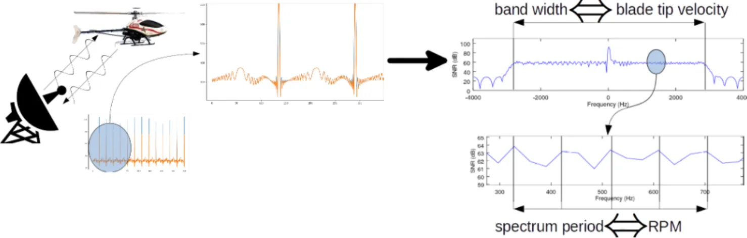
In its raw form, a radar signal is the result of an emitted wave reflected off a target, sampled at a given pulse repetition frequency (P RF), which yields a numerical time series of complex points(amplitude and phase) of intrinsic time-frequency nature [4]. Figure 2 shows how a mere fixed-time spectrum already allows for human interpretation and important feature extraction such as blade rotation speed Ω = RP M60 expressed in rad.s−1, Radar Cross-Section (RCS),
numberNb and lengthLb of blades and radial velocityVr. However, the extraction will likely
not be robust to real-world variations, thus nor will any subsequent classification algorithm.
2.1. A Physical Drone Model
In this section we introduce a simple yet expressive drone simulator. Firstly, the UAV is mod-elled by a discrete set ofNp scattering pointsdisseminated along its physical structure. Figure
3 shows the distribution of the scattering points, their reflection direction andRCS along with their temporal evolution. Note the model is 2-D as we consider the UAV to remain roughly in the same plane wrt the radar. Slight changes in inclination can be modelled by variations in the
RCS. Future work may include simulating roll, yaw and pitch and corresponding individual blade rotation speeds.
The Np scattering points moving in time yield a set of Np series of 2-D coordinates, which
are then fed to wave equations which return a temporal series of complex points. Finally, the signal is immersed in a noisy and cluttered environment. The noise is unavoidable white thermic noise from the sensing mechanism, the clutter sums up the influence the outside environment on the signal of interest; Billingsley’s model was used to model ground clutter [2]. The following section extends the simulator to account for unpredictible behavior, thereby introducing intra-class variety.
2.2. Dataset Generation
The simulator described above gives a deterministic output given one configuration. Real data are however subject to multiple variations even within one single measurement, whether it be responses to an unkown controller, alterations of the environment or the data acquisition itself,
Figure 2: Illustration of the simulated signal. Here, aP RF of8kHzon a signal of250msyields a time series of 2000 complex points, jointly drawn as modulus and real part. From a simple analysis of the featured spectrum, we can deduce three important characteristics of the UAV: rotation speedΩ, numberNb and lengthLbof blades. To the left: zoom-in of the original signal
(SN R = 50dB). Top right: complete Fourier transform (P RF = 8kHz), where we defineB
as the signal’s bandwidth (the plateau in the spectrum). Bottom right: zoom-in of the spectrum, where we defineν the observed period of its assumed periodicity. Then we haveν =NbΩand B = 4LbΩfe
c , which gives access to the three unkowns up to a hypothesis on the number of
blades, clean analysis pending. Note that for the sake of clear figures, the signal representation parameters such as as the P RF and the signal to noise ratio (SN R) were set to wishfully accomodating values. It is also important to point out that a gain in SN R of 10log(nf f t) ≈
15dB is achieved in performing the Fourier transform. The given SN R values take that gain into account.
Figure 3: Evolution of the scattering points and normals for the Vario, Phantom2 and S1000+ drones for a total simulation time of 250ms, of which we only illustrate the first 3ms (corre-sponding to 7 frames) for the sake of visual simplicity. The body is modelled as an isotropic reflector whereas blades are scattered with directional punctual reflectors in the direction of the normals, the length of which are proportional to the points’ reflectance. Notice the multi-copters’ helices alternatively turn clockwise and counter-clockwise. The 2-D scale is in meters; dimensions and distances are accurate wrt reality. Time goes from red to green.
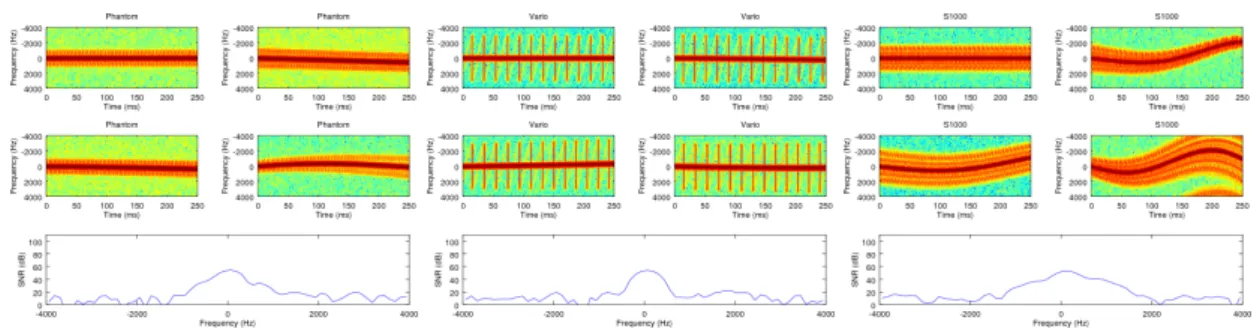
Figure 4: Spectrograms of noisy and uncluttered signals for the three drones mentioned above, from left to right: the Vario, the Phantom2 and the S1000+. Each group is organized as follows: four varying spectrograms of the same class are displayed; the top-left one always corresponds to a version constant in time. Below we plot an arbitrary time cut of one of the varying spec-trograms. Important parameters of the representation are: SN R = 40 dB, P RF = 8 kHz, Simulation time T = 250 ms, Nf f t = 64points and window overlap percentagepov = 50%.
Again, we take into account the gain in the Fourier transform and chose very forgiving config-uration parameters for the sake of visual clarity.
all in all tonon-cooperative behavior. These variations will define the intra-class disparity and thus the inter-class separability. We have chosen four parameters to model disparity:RCS,Vr,
Ωand flight curvature κ. Their values are found or estimated from drone specifications while their variations still need to be heuristically estimated in order to allow for more expressive sampling. For instance, theRP Ms inrad.s−1 are constrained as follows:
1. Vario:RP M ∈[1550; 1650]
2. Phantom:RP M ∈[4250; 5750]
3. S1000+:RP M ∈[3250; 4750]
Figure 4 shows intra and inter-class variations for the three drones Vario, Phantom2 and S1000+ for a given set of representation parameters. Intra-class variety is achieved by sampling pairs of drone parameter values in their acceptable ranges and linearly interpolating the resulting values in time. Visible temporal variations are as accurate as possible, although exaggerated, wrt re-ality. They exhibit discriminative behaviours which we hope to capture in learning algorithms. The reader may observe that the S1000+, under strong variations, bypasses the allowed band-width set by the P RF, which leads to the well known frequency folding phenomenon [19], or Doppler ambiguity, which in turn can hurt the representationss credibility as a robust one. Unfortunately, though we can set the parameter arbitrarily high in simulations (again, which we do here for the sake of visual clarity), real-world radar costs constrain theP RF to possibly sub-optimal thresholds.
3. Deep learning on radar signals
This section gives an overview of the base concepts of statistical learning developed in our classification algorithms. The simplest form of such algorithms is linear classification such as logistic regression [8], a stacking of which amounts to the simplest form of neural networks, the multi-layer perceptron (MLP) [16]. Contrary to MLPs, convolutional neural networks (CNNs, first introduced in [13] and popularized in [12]) exhibit shared and locally connected filters, ie convolutions, to exploit spatial locality in images.
3.1. Fully-convolutional networks for signal classification
Seeing a time-frequency representation as an image to be analyzed via a CNN constitutes a first attempt at deep radar classification. One first subtlety to handle is that choosing the same representation for input signals of potentially different lengths will lead to frequency dilution. The more natural solution is to use the same projection instead of the same representation, eg a spectrogam of fixed window size and overlap. This of course allows input data of different dimensions, not easily handled by standard CNNs. A natural bypass is to consider the problem as Multiple Instace Learning[20], or MIL. In this framework, one input data point is seen as a collection of multiple atomic instances of the same class. Concretely, we divide spectrogams in segments of equal length, which we denote as τ. We define these segments as noisemes
(in analogy to phonemes in speech recognition). The choice of τ is rather arbitrary, and is interpreted as the minimal duration one must observe the signal to accurately determine its class.
There exists a modification of CNNs which, although seemingly trivial, allows for semantic segmentation, ie pixel-level, or, in the case of radar classification, timestep-level classification:
Fully-convolutional networks (FCNs), introduced in 2016 by [14], where dense layers of size
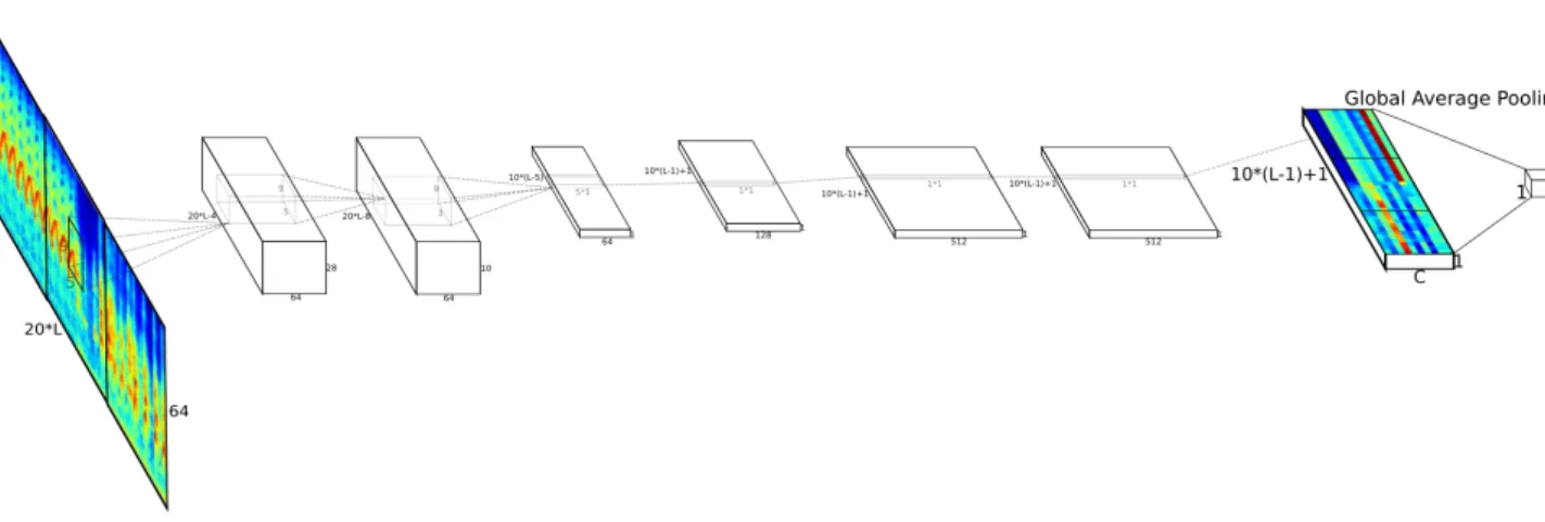
n are replaced with convolutional layers of size 1 and depth n. This artificial transformation is referred to in the paper as the “convolutionalization trick”. Additionally, a Global Average (or Max) Pooling (GAP) layer ensures correct dimensionality before final classification. Impor-tantly, the neural network now naturally deals with inputs of varying size and outputs temporal semantic feature maps when fed with longer signals. It is also worth noting the computational advantage of an FCN over, say, a sweeping of the original CNN on patches of data: indeed the architecture is highly optimized for parallel computation, which amounts to high training and testing speed on GPU, which allows for a variety of challenging applications such as image seg-mentation [10]. We design such a network, which we may name temporal fully-convolutional networkor TFCN, illustrated in figure 5.
The choice of hyperparameters for the network directly influences the inherent temporal pre-cision achieved by the TFCN, in particular the filter and pooling sizes and associated strides. Since the FCN is built upon the CNN classifier, the temporal feature map length lo equals 1
when given an input of lengthli =τ. We noteS(li) :=lo the global sizing function of the
net-work, composed ofLlayer-wise such functionsSl such thatSl(n) :=nl+1 =
j nl−kl+2pl sl k + 1, 5
Figure 5: The proposed architecture for radar signal segmentation,where the boxes represent the successive filter banks. Horizontal is time, vertical is frequency. C is the number of classes, ie 3 if we consider the Vario, Phantom2 and S1000+. In this example we feature a similar 10-class problem which has more visual interest. Contrary to Computer Vision, where the feature maps are spatial, our feature maps extend solely in time. We fix the noiseme lengthτ to 20 timesteps. Note that we omit pooling layers, strides, batchnorms, dropouts and non-linearities in the figure for visual simplicity.
wherenlandnl+1 are the input and output size at layerlandkl,plandslrespectively the filter
size, pad and stride at layerl. In the case of the proposed architecture 5, we have:
∀k ∈N∗, S(kτ) = SL◦ · · · ◦ S1(kτ) =b 5 2kτ −
5
2c+ 1 :=bf(k−1)τc+ 1 (1)
We introduced in the above equation 1 the finesse coefficient f which quantifies the super-resolution reached within a noiseme. By construction, f ∈ [1;τ], and its explicit formula is simply f = (QL
l=1sl)−1 (again, sl being the stride at layer l). For instance with τ = 20 and f = 52, we can classify the signal every8 timesteps instead of20, ie perform classification of controled precision. Overlapping receptive fields are one way to do so, we will see in the next section how neural networks can inherently support time dependency.
3.2. Recurrent neural networks for signal classification
Recurrent neural networks (RNNs) originally stem from standard perceptrons, but loop the inner states to learn on sequences of data rather than on individual, unordered points [7]. The core equation for RNNs is quite similar to that of perceptrons for it only adds the hidden state time dependency. RNNs do not naturally handle out time-frequency images as they are vector-based. Nonetheless, by considering the spectrogam no longer as an image but rather as a series of 1-D spectrums, which in essence it is, we face no more concern. In the recurrent framework, the finesse coefficientfis equal to its maximal valueτ as we are dealing with individual spectrums.
We can nonetheless relax fby adding a stride in the sequential spectrums, which amounts to subsampling the original time-frequency representation. In practice we implement a two-layer more sophisticated version of recurrent networks, Long Short Term Memory networks [11] (LSTM) which are able to learn longer time dependecies [3] and seem robust to slight time warpings in input signals [21], with 256 units at each layer.
4. Experiments
In this section we validate experimentally the classification of simulated data and study the influence of important parameters. To achieve this we build several datasets corresponding to different configurations.
4.1. Experimental setup
All datasets contain N = 1000examples for each of theC = 3classes, of which we reserve 25% for testing. We perform a 64-point sliding Fourier transform with Hamming windowing. We choose the noiseme length τ = 20 spectrogram timesteps, which corresponds to≈ 15ms
in real life (the choice is rather arbitrary though guided by the largest approximate period in all signals). Throughout the experiments we train the three classifiers (MLP, RNN and FCN) with the same strategy to remain consistent: stochastic gradient descent (SGD) with initial learning rateα= 0.5for the MLP, RMSProp [17] withα= 2e−3and decayβ = 1e−6for the RNN, and accelerated SGD withα = 4e−3and momentumµ= 0.9for the FCN. All optimizations are initialized by Glorot uniform sampling and run forK = 100epochs without early stopping nor cross-validation (except manual hyper-parameter finetuning). All learning rates are divided by2every25epochs. Models were implemented using the Keras [6] library with Tensorflow [1] backend and trained on a single Nvidia GTX 1070M GPU. Training a model takes less than an hour with all models.
4.2. General performance and robustness
First we train the classifiers multiple times on a standard configuration to evaluate overall perfor-mance and robustness to initialization to evaluate the simulator’s expressivity, seen in figure 6. Running the training20times for each classifier (we actually test three FCN architectures with different finesse coefficients), we observe consistent accuracy results, the most consistent being the FCN, which exhibits the smallest spread. In terms of accuracy, the MLP falls way behind the RNN and FCNs, which are close though the FCNs seem to generally perform better.
4.3. Impact of radar configuration parameters
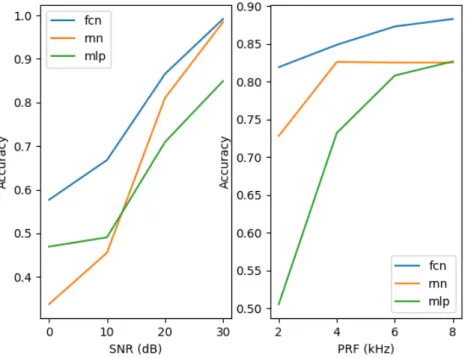
Here we train all models in different configurations; specifically we varySN RandP RF from extremely challenging to wishfully accomodating. Results are found in figure 7. The most
Figure 6: Classification accuracies for three learning models. Here we chose a setup of cluttered, noisy signals with SN R = 30dB on the left andSN R = 10dB to the right (P RF = 4kHz), which is more than reasonable from a practicioner’s point of view.
Figure 7: Performance of the learning models for increasingly good conditions. The graphs show intuitive behavior wrt the configurations.
lenging configuration being at SN R = 0dB and P RF = 4kHz, we nevertheless achieve
≈ 58% with the FCN, versus total confusion (≈ 33%)) with the MLP. Note this is an unreal-istically challenging configuration, as an SN R of0dB means an original signal to noise ratio before Fourier transform of≈ −15dB. Again, the FCN seems to be more robust to bad quality signals, although this should eventually be validated on real data.
5. Conclusion
We have introduced an expressive simulator for blade-propelled engines such as drones with sufficiently realistic variational characteristics, which we have shown to be suited for machine learning on three distinct models: MLPs, RNNs and FCNs, which in turn we have experimen-tally validated to perform well even in harsh simulation conditions. We have furthermore jus-tified the assumption that RNNs and FCNs that, because they can inherently learn temporal fluctuations, are particularly appropriate to the task of radar classification as they are able to handle signals of increasing length over time. Further developments for the simulator include its refinement to real-life subtleties and its extension to other kinds of UAVs. As for machine learning, the temporal architectures pave the way to more difficult tasks than classification, for instance detection, labelling and segmentation.
References
[1] M. Abadi, P. Barham, J. Chen, Z. Chen, A. Davis, J. Dean, M. Devin, S. Ghemawat, G. Irving, M. Isard, M. Kudlur, J. Levenberg, R. Monga, S. Moore, D. G. Murray, B. Steiner, P. Tucker, V. Vasudevan, P. Warden, M. Wicke, Y. Yu, and X. Zheng. TensorFlow: A System for Large-scale Machine Learning. InProceedings of the 12th USENIX Conference on Operating Systems Design and Implementation, OSDI’16, pages 265–283, Berkeley, CA, USA, 2016. USENIX Association. [2] D. K. Barton. Low-angle radar tracking. Proceedings of the IEEE, 62(6):687–704, June 1974. [3] Y. Bengio, P. Simard, and P. Frasconi. Learning long-term dependencies with gradient descent is
difficult. IEEE Transactions on Neural Networks, 5(2):157–166, Mar. 1994.
[4] V. Chen, F. Li, S.-S. Ho, and H. Wechsler. Analysis of micro-Doppler signatures. IEE Proceedings - Radar, Sonar and Navigation, 150(4):271, 2003.
[5] V. C. Chen, F. Li, S.-S. Ho, and H. Wechsler. Micro-Doppler effect in radar: phenomenon, model, and simulation study. IEEE Transactions on Aerospace and electronic systems, 42(1):2–21, 2006. [6] F. Chollet et al. Keras. https://keras.io, 2015.
[7] J. Collins, J. Sohl-Dickstein, and D. Sussillo. Capacity and Trainability in Recurrent Neural Net-works. arXiv:1611.09913 [cs, stat], Nov. 2016. arXiv: 1611.09913.
[8] D. R. Cox. The regression analysis of binary sequences. Journal of the Royal Statistical Society. Series B (Methodological), pages 215–242, 1958.
[9] J. J. M. De Wit, R. I. A. Harmanny, and P. Molchanov. Radar micro-Doppler feature extraction using the singular value decomposition. InRadar Conference (Radar), 2014 International, pages 1–6. IEEE, 2014.
[10] T. Durand, T. Mordan, N. Thome, and M. Cord. WILDCAT: Weakly Supervised Learning of Deep ConvNets for Image Classification, Pointwise Localization and Segmentation. InIEEE Conference on Computer Vision and Pattern Recognition (CVPR 2017), Honolulu, HI, United States, July 2017. IEEE.
[11] S. Hochreiter and J. Schmidhuber. Long Short-Term Memory. Neural Comput., 9(8):1735–1780, Nov. 1997.
[12] A. Krizhevsky, I. Sutskever, and G. E. Hinton. Imagenet classification with deep convolutional neural networks. InAdvances in neural information processing systems, pages 1097–1105, 2012. [13] L. a. B. Y. a. H. P. LeCun, Yann and Bottou. Backpropagation Applied to Handwritten Zip Code
Recognition. 86(11):2278–2324.
[14] J. Long, E. Shelhamer, and T. Darrell. Fully convolutional networks for semantic segmentation. In Proceedings of the IEEE Conference on Computer Vision and Pattern Recognition, pages 3431– 3440, 2015.
[15] P. Molchanov, R. I. Harmanny, J. J. de Wit, K. Egiazarian, and J. Astola. Classification of small UAVs and birds by micro-Doppler signatures. International Journal of Microwave and Wireless Technologies, 6(3-4):435–444, June 2014.
[16] F. Rosenblatt. The perceptron: A probabilistic model for information storage and organization in the brain. Psychological review, 65(6):386, 1958.
[17] S. Ruder. An overview of gradient descent optimization algorithms. arXiv:1609.04747 [cs], Sept. 2016. arXiv: 1609.04747.
[18] V. Schmidlin, G. Favier, R. Fraudt, and V. Schmidlin. Multitarget Radar Tracking with Neural Networks. IFAC Proceedings Volumes, 27(8):621–626, July 1994.
[19] Shannon C. E. A Mathematical Theory of Communication. Bell System Technical Journal, 27(3):379–423, July 2013.
[20] N. Takahashi, M. Gygli, and L. Van Gool. AENet: Learning Deep Audio Features for Video Anal-ysis. arXiv:1701.00599 [cs], Jan. 2017. arXiv: 1701.00599.