INTERMEDIATION AND VERTICAL INTEGRATION Mitchell Berlin
Federal Reserve Bank of Philadelphia Loretta J. Mester
Federal Reserve Bank of Philadelphia, and
The Wharton School, University of Pennsylvania
Revised: February 1998 Original Version: October 1997
We thank the participants of the Conference on Comparative Financial Systems, sponsored by the Federal Reserve Bank of Cleveland and the Journal of Money, Credit, and Banking, Joe Haubrich, George Mailath, Andy Winton, our discussant George Pennacchi, and an anonymous referee for very helpful comments.
The views expressed in this paper do not necessarily represent those of the Federal Reserve Bank of Philadelphia or of the Federal Reserve System.
Mitchell Berlin
Federal Reserve Bank of Philadelphia and
Loretta J. Mester
Federal Reserve Bank of Philadelphia, and
The Wharton School, University of Pennsylvania
Abstract
Competition in retail and wholesale funding markets affect the incentive for originators (like investment bankers) and fund managers (like mutual funds) to form integrated intermediaries (banks). Independent firms integrate both to produce higher yielding, illiquid assets and to suppress competition in retail markets. In addition to the higher return on illiquid assets, three factors increase the incentive to integrate. First, homogeneous savers lower the costs of producing illiquid assets and increase
competition in retail markets. Second, fund managers’ market power in wholesale markets increases competition in retail markets. Finally, more certain aggregate savings reduces the costs of producing illiquid assets.
Introduction
Modern models of intermediation have usually contrasted two stylized setups for transferring funds from individual savers to businesses. In the first setup, savers provide funds directly to firms by1 buying their securities. In the second, intermediaries such as banks channel savings from individuals to firms. Actually, in modern financial markets the lion’s share of financial transfers from ultimate savers to borrowers, even those that our models would view as “direct” transactions in securities markets, are mediated by firms. Borrowers seeking funds typically approach originators, specialized financial firms such as investment banks to market their securities. On the other side of the market, individuals place their savings with fund managers, other firms such as mutual funds and pension funds. Thus, a typical transaction in the direct securities market actually involves transactions in three different markets: the market where businesses meet originators, the market where originators sell securities to fund managers (which we call the wholesale securities market), and the market where savers meet fund managers (which we call the retail securities market).
From this viewpoint, intermediation is a form of vertical integration, in which potentially separate originators and fund managers choose to integrate and form intermediaries, rather than transact through markets. One benefit of viewing intermediation this way is that it highlights the question of2 whether competitive conditions in these markets affect the incentive to form intermediaries. This is a question that previous models of intermediation have largely ignored, and it is the question we address in this paper.3
In our model, originators and fund managers integrate to form intermediaries for two reasons. The first is that prior coordination between the originator and a fund manager is needed to fund high yielding, but illiquid, assets. Thus, the incentive to integrate is affected by the relative costs and benefits of producing illiquid assets. The second motive for integration is to weaken competition in retail funding markets. In our model, integrated intermediaries can arise either because they are more efficient than
nonintegrated firms or because they are better at suppressing competition for savers’ funds when competitive forces in retail markets are strong.
The main tradeoffs in our analysis depend on three factors, in addition to the return differential between illiquid assets and liquid assets. The second factor is the degree of saver heterogeneity, which affects both the return from producing illiquid assets and the degree of competition in retail markets. Viewing an asset’s liquidity as the ease with which it can be matched with multiple types of liabilities, we show that when savers are very heterogeneous in their tastes for savings vehicles with different return and transactions features, illiquid assets are more costly to produce and, thus, the profitability of
integration is lower. In addition, when savers are very heterogeneous, competitive forces in retail markets tend to be weak. Thus, saver heterogeneity also reduces the incentive to integrate to dampen competition at the retail level.
The third factor affecting the motive for intermediaries to integrate is the relative market power of originators and fund managers in the wholesale funding market. There are numerous examples of institutional changes that have significantly affected competitive conditions in wholesale funding markets. For example, there is empirical evidence that the growth of large institutional savers, such as pension funds in the 1980s, may have reduced the market power of investment bankers (see Bloch, 1986). Similarly, the development of multiple, competing investment banks with the ability to distribute junk bonds in the 1990s contrasts strongly with the near dominance of a single investment bank (Drexel) in the 1980s. In our model, when independent fund managers have a lot of market power vis a vis originators, the resulting high returns on the securities they purchase induce them to compete more fiercely for savers’ funds. This competition transfers contractual surplus to savers, which enhances the incentive for independent firms to integrate to suppress competition in the retail market.4
The final factor affecting the incentive to integrate is uncertainty about aggregate savings. A higher likelihood of an aggregate funding shortage raises the costs of originating illiquid investments,
thus reducing the benefits of intermediation. In the presence of an aggregate funding shortage,
originators find it difficult to meet commitments to seek funds for projects without scouring the market for the savings of many different types of savers. Thus, originators of illiquid assets are forced to pay a high cost to attract funds from savers whose own preferred liabilities are poorly matched to those of the intermediary
The paper proceeds as follows. In Section 1 we outline and discuss the model. In Section 2 we present equilibrium outcomes in two alternative market structures, one a vertically integrated market and the other a market in which originators and fund managers remain separate. We present our main results in Section 3, providing conditions in which each of the market structures arises. Section 4 concludes and suggests some directions for future research.
1. The Model
1.1. Agents and Technology
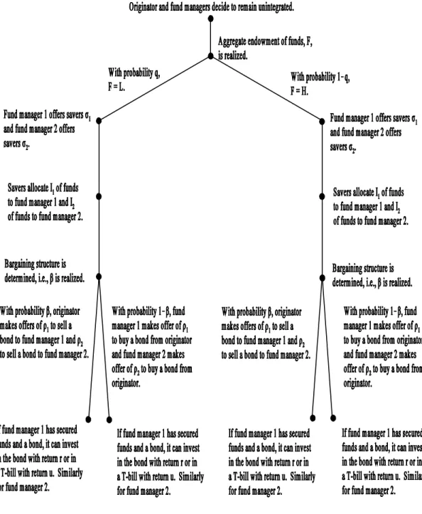
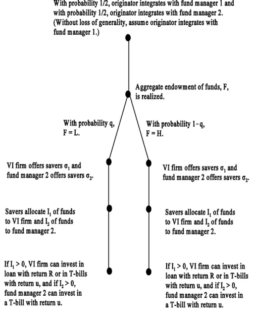
Figures 1, 2, and 3 show the structure of the game. There are three types of agents: originators, fund managers, and savers.
The originator. There is one originator who is both a specialist in identifying profitable firms and making commitments to secure financing for the firms identified. As a stand-alone firm, the
originator can be thought of as an investment banker. Although all agents in the economy have access to a T-bill that pays return u per unit of funds invested, the originator has exclusive access to higher
yielding investments. Specifically, the originator makes a mutually exclusive choice between two types of investments. We think of the two types of investments as a loan, which is highly illiquid but yields a high return, R, and a bond, which is highly liquid but yields a relatively low return, r, with R > r > u. (We will discuss the precise meaning of liquidity in the section immediately following.) For simplicity, we assume that the return function is linear in the funds invested, I, so, for example, an originator producing bonds generates securities with return rI. All investments yield their returns at the end of the
game.
A final characteristic of the investment technology is that there is a minimum investment size Imin. This is a simple way of capturing the originator’s binding contractual commitment to seek financing for borrowing firms, although we do not model equilibrium contracting between firms and the originator explicitly. Indeed, the firms that are the ultimate source of the asset returns remain in the background5 throughout the paper, and we do not model the competitive conditions in the market for originators’ services.
Fund managers. There are two fund managers, indexed by m0 {1,2}. As a stand-alone firm, the fund manager can be thought of as a mutual fund or a pension fund. The primary function of each fund manager is to create a savings vehicle with return and transactions features attractive to savers with particular preferences. Thus, we think of the various fund managers as having differentiated liabilities, each with a single type of liability. (Of course, the fund managers’ liabilities are viewed as assets by the savers who hold them.) After the total volume of savers’ funds in the market becomes known, fund managers compete for these funds and then use these funds to invest in assets.
One of the key features of our model is a technological restriction on the conditions permitting the matching of types of assets and liabilities. We define the liquidity of an asset as the ease with which it can be matched with multiple types of liabilities. In fact, we consider the polar case in which assets are either perfectly liquid or completely illiquid. So, for example, if the originator chooses the liquid bond it can be sold to fund managers 1 and 2 in any proportions without deadweight costs. On the other hand, an illiquid asset is one that can be matched with only one type of liability. This means that at the beginning of the game, the originator of a loan and one of the fund managers must make an irrevocable match if that manager wishes to hold the loan in its portfolio. We assume that each fund manager has an equal probability of being the one that integrates with the originator, provided the originator and
Savers. There is a continuum of savers in our model, distributed on the unit interval [0,1]. These savers can be one of two types, indexed by i0 {1,2}. We assume that savers cannot contract directly with originators; for anything other than T-bills, savers must place their savings in one of the two funds. Savers hold the liabilities of a fund, m, both for the promised interest rate factor ( m) and for other characteristics of the liability that affect the saver’s preferences. In particular, we assume that the saver receives added utility, k, when holding utilities well matched to her preferences. Thus, the savers’ utility function can be written:
vi = ( + k)I , i = m, (1)
m m i
= m iI , i û m,
where I is the amount invested by savers with fund manager i. This is a simple way to capture the ideai
that savers are concerned about features like transaction services, maturity, or the availability of investment advice and other collateral services, in addition to the expected return on their savings. We will often refer to those savers whose tastes are well matched to fund manager m’s liabilities as the fund manager’s home market. Note that higher k corresponds to greater heterogeneity among savers.
Savers’ aggregate endowment of funds, F, is a random variable that is realized just before period 1, with F 0 {L,H}, L < H, and funds are divided equally between the two types of savers. The prior probability of the scarce funding state (i.e., F = L) is q while the prior probability of the plentiful funding state (i.e., F = H) is 1! q. These probabilities are common knowledge before the game begins, and the actual realization of the funding state becomes common knowledge before fund managers compete for savings. To exclude uninteresting cases, we make the parametric restrictions that when funds are scarce, aggregate funds are sufficient to meet the minimum funding requirement, but home funds are not. That is, we assume:
Imin < L < H, and (2)
1.2 Market structures and timing
There are two possible market structures, the non-integrated market (NI) and the vertically integrated market (VI).
The NI Market. In an NI market, the originator and the fund managers decide to remain separate firms and the originator chooses the bond as his investment. Figure 2 shows the structure of the rest of the game. After the realization of F, the two fund managers act as Bertrand competitors in the retail funding market, the market in which fund managers secure savers’ money. The fund managers’ offers for savers’ funds, and , are guaranteed contractual returns in the sense that they must be paid1 2
even if portfolio returns are insufficient to cover the contractual guarantee. The offers, and , are7
1 2
determined by a “button auction” (see Milgrom and Weber, 1982). Each manager makes its initial offer, which subsequently rises until the fund manager decides it wants no further increase; each fund manager observes the offer price at which the other drops outs. Once the final offers are made, savers allocate their funds to the two fund managers, with fund manager m receiving I of funds. Note that eachm
originator offers only a single return. Thus, we assume that fund managers cannot price discriminate. Subsequently, the wholesale funding market, where originators sell assets to fund managers, opens. We adopt a stylized model of competition in the wholesale funding market that is simple, but nonetheless permits us to highlight the relative market power of originators and fund managers.
Specifically, we assume that with probability the originator makes once-and-for-all offers of { , } to1 2
the fund managers and that with probability 1! , the two fund managers make uncoordinated once-and-for-all offers { , } to the originator, where 1 2 m is fund manager m’s return per dollar of the bond purchased. Thus, measures the market power of the originator. Using the previous examples from the Introduction, an increase in the weight of institutional savers in securities markets in the 1980s or the shift away from a junk bond market dominated by Drexel toward one where multiple investment bankers have the capability of marketing junk bonds would both be viewed as a decrease in in our model.
The VI Market. In the VI market structure, the originator and a randomly chosen fund manager have integrated to form a bank. In contrast to an incomplete contracting perspective, in which the fund manager’s and originator’s interests conflict, we assume the vertically integrated firm acts as a unitary, profit-maximizing firm.8
The primary purpose of vertical integration is to permit the originator to choose the illiquid investment. We assume that the higher returns of the illiquid investment come at a cost: the originator and a single fund manager must make a prior commitment at the outset for the higher yielding illiquid investment to be chosen. In turn, this limits the marketability of the investment. We consider the polar case in which the asset cannot be sold to another fund manager at any cost. Since this is an essential assumption—and since we do not model the underlying frictions explicitly—some further discussion is necessary. We view the underlying connection between illiquidity and exclusivity as arising from two causes.
The first connection is well established in the banking literature. Although our model does not incorporate information asymmetries and adverse selection effects, it would not be difficult to introduce these as the underlying source of illiquidity. In this interpretation, illiquidity arises from private
information, and vertical integration involves the creation of a specialized monitoring technology that is costly to duplicate. Then we would identify liquid securities as assets for which private information is less of a problem, perhaps standardized assets or securities floated by firms for which substantial public information exists.
A second interpretation has not been as extensively considered in the literature on
intermediation. If we think of our bonds as standardized assets, numerous strategies exist to facilitate the matching of dissimilar assets and liabilities at relatively low cost. The use of futures and options for hedging purposes, and more recently the growing sophistication of the technology for securitizing assets,
all tend to break the links between the payoff characteristics of assets held in portfolio and the types of liabilities that might profitably be matched with those assets. So a standardized asset can be divided up and sold to different fund managers at low cost.
This is not true of complicated or highly idiosyncratic assets. For such assets the matching of asset and liability characteristics may also involve the use of derivative securities, but we expect that a higher degree of prior coordination is necessary. And even then, we do not expect as many degrees of freedom in matching disparate assets and liabilities. Good examples of the types of coordinating mechanisms we have in mind are banks’ traditional internal control structures: the asset-liability committee and the loan review committee. These internal institutions impose a high degree of prior coordination on the asset and liability production activities of a commercial bank and help to mitigate (at a cost) any conflicts of interest within the intermediary. Although complicated and idiosyncratic assets9 may have high yields, the necessary degree of coordination restricts the liquidity of the assets. Needless to say, coordination imposes resource costs as well as opportunity costs, so we may think of the higher return on loans, R, as net of these coordination costs.10
Figure 3 shows the structure of the rest of the game after the decision to integrate. Without loss of generality, we have assumed in the figure that fund manager 1 integrates with the originator; there is a similar subgame if fund manager 2 integrates. This subgame is similar to the nonintegration subgame except that now fund managers do not buy assets from the originator—the integrated fund manager has access to the loan and the nonintegrated fund manager has access only to T-bills.
2. Equilibrium
To solve for the equilibrium of the game we use backward induction. We will first consider the nonintegration subgame (Figure 2) and then the vertical integration subgame (Figure 3). Finally, we will analyze the decision to integrate.
2.1. Equilibrium in the NI market
First consider the game in the wholesale funding market in the nonintegration subgame. Proposition 1: In equilibrium in the NI market, when the originator makes the offer to fund managers in the wholesale market, it offers = = u per unit of funds. And when the fund managers1 2
make offers to the originator in the wholesale market, they offer = = r.1 2
Proof. The fund managers have an outside option, T-bills, that yield u per dollar invested. Thus, when the originator makes the offer, it offers each fund manager u (and the originator’s own return is r ! u). When the fund managers have the bargaining power, they capture the surplus and therefore offer the originator a return of 0 per unit invested (while they receive the full return on the bond, r). This is
true whether funds are scarce or plentiful. QED
Proposition 2: In equilibrium in the NI market, the funds managers’ offers to savers and the savers’ allocations of funds are as follows:
= = u, I = I = F/2, F = L or H, if u + (1! )r ! 2k < u, (4)
1 2 1 2
= = *, I = I = F/2, F = L or H, if u + (1! )r ! 2k > u, (5)
1 2 1 2
where * / u + (1! )r ! 2k.
Proof. Given proposition 1, a fund manager’s expected return to offering m is [ u +
(1! )r ! m]I ( , ), where I ( , ) is the amount of funds it secures given the offers being made. m 1 2 m 1 2
Note that * / u + (1! )r ! 2k is that price such that a fund manager is indifferent between paying that price and receiving only its home market funds and paying * + k and receiving all the funds; in other words, [ u + (1! )r ! *]F/2 = [ u + (1! )r ! ( * + k)]F. If his opponent’s offer is fixed at , u # , then þ > 0 such that a fund manager would prefer offering + k + and gaining all the funds to offering and gaining half the funds, if and only if, < *. Also note that if his opponent offers , then in equilibrium, a fund manager would never offer between and +k, since this would result in his gaining only half the funds, and he would do strictly better by offering .
Consider the button auction. First, examine symmetric equilibria. There will be no equilibrium where the fund managers each receive half of the funds in the market but are offering different prices, since the manager offering the higher price can always do better by dropping out at a slightly lower offer than its current offer. It would retain half of the funds in the market but pay a lower price for them.
Now consider symmetric equilibria in which the fund managers split the market for funds and offer the same price. Examine whether ( , ) = (u,u) is an equilibrium. If fund manager 1 quits at offer1 2
u, would fund manager 2 quit at u or keep going? It would quit at u, as long as u $ *, i.e., if u + (1! )r ! 2k # u, by the definition of *. Would fund manager 1 quit before u? No, because any offer lower than u secures zero funds (since savers get u by investing in T-bills). Thus, when u + (1! )r ! 2k < u, ( , ) = (u,u) is the unique symmetric equilibrium.1 2
Now assume u + (1! )r ! 2k > u and examine whether ( , ) = ( *, *), is an equilibrium,1 2 where */ u + (1! )r ! 2k. Suppose fund manager 1 quits at *, then by the definition of *, fund manager 2 has no incentive to raise his offer over * to gain all the funds. Would fund manager 1 want to quit at an offer, , less than *? No, because if he did, then þ > 0, such that fund manager 2, seeing where fund manager 1 stopped, would raise its offer to + k + and gain all the funds, leaving fund manager 1 with zero profits (which is strictly less than he would receive by matching fund manager 2’s offer). In particular, choose , such that < ( * ! )/2. Thus, when u + (1! )r ! 2k > u, ( , ) = ( *,1 2
*) is the unique equilibrium. It is unique, since if one of the fund managers stops at any price < *, there exists a > 0, such that the other fund manager would want to raise its price to + k + and gain all the funds. But given this, the first fund manager would not want to stop at that . Similarly, there can be no equilibrium with both fund managers making offers greater than *, since if one of the fund managers did so, the other could gain by stopping at a slightly lower offer that is still greater than *. This will be profitable, since at this slightly lower offer, they each still receive half of the funds—the other manager will not try to capture all of the funds, since the offer is still greater than *.
Finally, it remains to show that there are no asymmetric equilibria, with one fund manager getting all the funds and the other getting none. If a fund manager stops at any offer < *, then the other fund manager has the incentive to offer + k + to receive all the funds. Thus, any asymmetric equilibrium with one fund manager getting all the funds will involve its making an offer greater than * + k. But this fund manager would be better off offering * and splitting the market for funds with the other fund manager, since for any price ˆ > * + k, [ u + (1! )r ! *]F/2 > [ u + (1! )r ! ˆ]F. QED
Discussion. There are several things to note about the equilibrium. First, whether funds are scarce or plentiful, the two fund managers always split the market for funds, and savers are always matched with their most preferred liability in an NI equilibrium. In addition, all available funds are fully invested in the intermediated asset.
Note that when u + (1! )r ! 2k > u, the equilibrium rates in the retail market will depend on the gross return on the asset, r, the savers’ utility from being matched with her preferred liability, k, and the relative market power of the originator and fund managers in the wholesale market, . Intuitively, fund managers compete more aggressively for savers’ funds when expected returns are high compared to the savers’ cost of holding a mismatched liability. When savers are highly differentiated (i.e., when k is high), or when assets are relatively low paying (i.e., when r is low), or when fund managers have less bargaining power vis a vis the originator (i.e., when is high), it is relatively unprofitable for a fund manager to attempt to lure savers to accept a less preferred liability by offering a high return. Fund managers make no attempt to invade each other’s home market and each acts as a local monopolist. It will be convenient to refer to this region, i.e., when u + (1! )r ! 2k < u, as the local monopoly region.
When savers are relatively homogeneous (i.e., when k is low), or liquid assets are very high paying, (i.e., r is high), or when fund managers have more bargaining power against the originator (i.e., is low), fierce competition drives the expected return to each fund manager down to 2k(F/2) = 2k, with savers capturing nearly all of the expected return from the asset. We will refer to this region, i.e, when11
u +(1! )r ! 2k > u, as the competitive region. 12
Profits in the NI market. Using Propositions 1 to 3, the expected profits of the players in the nonintegration subgame can be derived immediately. Let (NI) denote the agents’ expected profits ink
the nonintegrated market, with k = o for originator and k = m for fund manager. Then using Proposition 1 we have:
(NI) = q (r ! u)L + (1!q) (r ! u)H, (6)
o
(NI) = q(1! )(r ! u)L/2 + (1!q)(1! )(r ! u)H/2, if u + (1! )r ! 2k < u, (7)
m
= qkL + (1!q)kH, if u + (1! )r ! 2k > u. (8)
The joint expected profits of the nonintegrated originator and the two fund managers are:
(NI) = q(r ! u)L + (1!q)(r ! u)H, if u + (1! )r ! 2k < u, (9)
J
= q[ (r ! u) + 2k]L + (1!q)[ (r ! u) + 2k]H, if u + (1! )r ! 2k > u. (10)
In the NI market, the originator captures the full contractual surplus (r ! u) whenever it makes the once-and-for-all offer, which happens with probability . Since no fund manager has to seek out funds beyond its home market, the linearity of the investment function and the assumption that r > u ensure that bonds use up all available savings in the NI market. Thus, funding occurs at level L with probability q and at level H with probability (1!q) as shown in expression (6). With probability (1! ), the fund managers capture the contractual surplus in the wholesale funding market, but as we noted in the discussion of Proposition 2, sufficiently high asset returns and a low degree of saver heterogeneity lead to aggressive competition. In the competitive region, the fund managers end up transferring most of the contractual surplus to savers.
2.2 Equilibrium in the VI market
Funding managers 1 and 2 are equally likely to be the one that integrates with the originator. Therefore, without loss of generality, assume that it is fund manager 1 that integrates with the originator. Since the intermediated asset is simply transferred within the intermediary, instead of being sold in a wholesale market, there is no explicit return, .1
To simplify our presentation of results we make one further parametric restriction. Specifically, we assume that saver heterogeneity is low enough that the gross surplus from financing the loan with funds outside the home market is always positive, that is,
R > u + k.13 (11)
Again, we will solve the vertical integration subgame (see Figure 3) using backward induction. Proposition 3: In equilibrium in the VI market, the vertically integrated firm (i.e., the bank) offers savers per dollar of funds and secures I dollars of funds, where:1 1
(i) If F = L, = u + k, I = L. (12) 1 1 (ii) If F = H, = u, I = H/2, if R < u + 2k, (13) 1 1 = u + k, I = H, if R > u + 2k. (14) 1 1
Th nonintegrated fund manager 2 does not operate. Type 2 investors hold F ! I dollars worth of funds in1
T-bills.
Proof. Since fund manager 2 does not have a project available to it, it is indifferent between attracting savers’ funds by offering = u, or else staying out of the market. We assume that the fund2
manager stays out of the market. When F = L, by assumption (3) that L/2 < Imin, the bank must attract funds from savers outside its home market in order to meet its funding commitment. Thus, it will offer savers the lowest price that attracts the outside funds, = u + k, and then invest L in the project, since1
[R ! (u+k)]L > [R ! (u+k)]Imin, by assumption (2), that Imin < L, and assumption (11), that R > u+k. Remember that we have assumed that the bank cannot price discriminate and offer its home customers u and outside customers u + k.
When F = H, then by assumption (3), H/2 > Imin, so the bank need not attract funds from outside its home market in order to meet its commitment. The bank will want to attract and invest all the funds if it is profitable to do so, i.e., if and only if, [R ! (u + k)]H > [R ! u ]H/2, i.e., R > u + 2k. Otherwise, it
offers = u to attract its home funds and invests H/2.1 QED
Discussion. Note that when funds are abundant, the bank can decide whether to limit the scale of investment, setting I = H/2, by paying a low cost of funds, = u, or to invest fully in the loan but pay1 1
a higher cost of funds, = u + k. By expressions (13) and (14), the bank is more likely to limit1
investment if the loan return, R, is relatively low, and if savers are very heterogeneous, i.e., k is high. We will refer to the region in which the bank chooses to invest H/2, i.e., when R < u + 2k, as the limited investment region, and to the region in which the bank invests H, i.e., when R > u + 2k, as the full investment region.
Profit functions. Using Proposition 3 and assumption (3) that L/2 < Imin < H/2, we can write the joint expected profits of the vertically integrated originator and the two fund managers as:
(VI) / q(R ! u ! k)L + (1!q)(R ! u)H/2, if R < u + 2k, (15)
J
(VI) / q(R ! u ! k)L + (1!q)(R ! u ! k)H, if R > u + 2k. (16)
J
3. When Will the Firms Choose to Vertically Integrate?
We have solved the nonintegration and vertical integration subgames. It remains to be determined which subgame will be played in equilibrium. We proceed by comparing the agents’ expected profits in each of the subgames.
The following proposition shows that the VI market structure is the equilibrium market structure, if and only if, the joint expected profits of all firms in the market exceed their joint expected profits as
stand-alone firms.
Proposition 4: The originator and portfolio manager 1 merge, if and only if: = (VI) J ! (NI) J $ 0,
where,
(NI) / (NI) + (NI) + (NI).
J o m m
1 2
Proof: Begin with an NI market structure and consider the firms’ incentives to integrate. Define (VI) as the profits of the integrated firm that are allocated to the originator and (VI) as the profits of
o m
the integrated firm that are allocated to the fund manager that has integrated. Suppose that the originator proposes integration and recall that each fund manager has a 1/2 probability of receiving the offer. Also recall that the nonintegrated fund manager receives zero profits whenever it operates in the VI market. Then the expected profits of manager i in a VI structure is 1/2 m(VI) + 1/2@0 = 1/2 m(VI). Thus, manager i would opt to integrate if and only if,
1/2 m(VI) $ m(NI),
i
i.e., m(VI) $ 2 m(NI) = m(NI) + m(NI)
i 1 2
since the profits of the fund managers are equal in the NI market. The originator can profitably make such an offer, if and only if,
(VI) $ (NI).
o o
If both conditions hold, then
(VI) + (VI)$ (NI) + (NI) + (NI)
o m o m m
1 2
i.e., (VI) J $ (NI), J
i.e., $ 0.
And if $ 0, there is an allocation of total profits of the VI firm between the originator and the fund
manager that will induce both to want to integrate. QED
the joint profits of the firms in the market, which may not equal total contractual surplus in the market. Specifically, savers’ consumer surplus does not enter into firms’ decision to integrate.14
3.1 The equilibrium market structure
We can now turn to conditions for the VI market structure to arise, that is, we now state the conditions under which > 0. Equations (9), (10), (15), and (16), which describe the firms’ joint profits in the nonintegrated and integrated markets, respectively, indicate that will differ depending on whether the parameters imply the limited or full investment region (i.e., R < u + 2k or R > u + 2k) and whether they imply the local monopoly or competitive region (i.e., u + (1! )r ! 2k < u or u + (1! )r ! 2k > u. (Note that the restricted investment region and competitive region cannot hold simultaneously.)
= q[(R ! u ! k) ! (r !u)]L + (1!q)[(R ! u)(H/2) ! (r !u)H] if R < u + 2k (17) = q(R ! r ! k)L + (1!q)(R ! r !k)H if R > u + 2k
and u+(1! )r ! 2k < u (18) = q[(R ! u) ! (r !u) ! 3k]L + (1!q)[(R ! u) ! (r !u) ! k]H if R > u + 2k
and u+(1! )r ! 2k > u (19)
The underlying intuition as to whether the VI market structure or NI market structure will arise in equilibrium is that there are two broad factors governing the incentive to integrate: (i) the costs and benefits of producing illiquid assets, and (ii) the gains from suppressing competition in retail funding markets.
We begin with Proposition 5, which provides a sufficient condition for the VI market to arise on efficiency grounds alone, that is, without regard to competitive conditions in retail markets.
Proposition 5: R! r > k Y > 0. (20)
Proof: See the appendix.
throughout is that illiquid investments have a higher return than liquid investments. This advantage to the bank can be measured by R ! r per dollar of funds invested by the bank. The basic cost of producing illiquid assets is that the bank is forced to pay an additional cost, k, for funds to attract savers outside its home market, and the bank responds to this cost in one of two ways. Either the bank limits investment so that it can rely on home market funds or it pays the extra cost to attract funds outside the home market.
Of course, when funds are scarce, to meet its financing commitment, the bank is forced to attract funds from beyond its home market, and since the bank cannot price discriminate, it invests all available funds, L, but pays the mismatching cost, k. However, when funds are plentiful, the bank does have a choice of whether to limit its investment, and the bank limits investment, if and only if, R < u + 2k.
Proposition 5 says that when the per unit benefit of illiquidity exceeds the cost, integration is profitable. This is most obvious in the full funding region, in which both market structures yield the same total level of investment. Here, the bank’s profits must exceed the total expected profits in the NI market by at least R ! r ! k per unit of funds invested. But Proposition 5 also holds when the bank15 limits investment, because the reason that the bank limits investment is that it is more profitable to avoid the mismatching costs by staying in its home market. Thus, R ! r > k is a sufficient condition for
integration to be profitable.
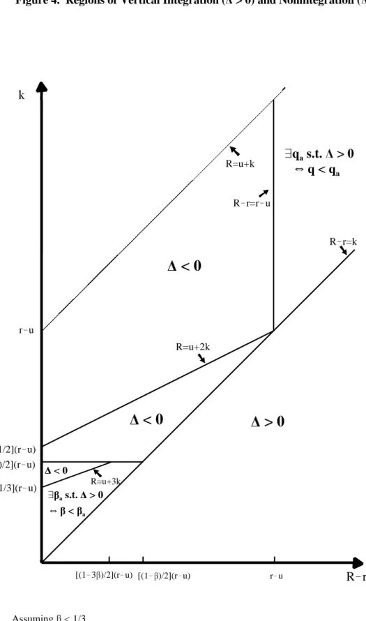
Proposition 6 is presented in tabular form to make it easier to read. This proposition describes the equilibrium market structure when R ! r < k, that is, when the higher return on the loan (compared to the bond) is less than the bank’s higher cost of funds if the bank seeks funds outside its home market.
Proposition 6. If R ! r < k, then the sign of is described in the following table:
Limited Investment Region Full Investment Region
R < u + 2k R > u + 2k
Local Monopoly Region (i) R ! r < r ! u Y < 0
u + (1! )r ! 2k < u (ii) R ! r > r ! u Y > 0 þ q s.t. > 0 a ] q < qa
Competitive Region (i) R < u + 3k Y < 0 u + (1! )r ! 2k > u (ii) R < u + 3k Y
þ s.t. > 0 a ] < a
Proof: See the appendix.
Discussion. Consider first, the upper left cell. In the limited investment region the bank prefers to limit investment to its home market whenever feasible. Indeed, as long as originators act as local monopolists in the VI market—so only efficiency considerations enter the decision whether to
integrate—vertical integration can be profitable only when the bank does actually restrict investment and so avoids paying the higher cost of funds outside its home market. This follows directly from the condition R ! r < k.
The conditions in the top left cell are intuitive. When R ! r < r ! u, the higher return on the loan per unit invested by the bank, R ! r, is outweighed by the opportunity cost of a limited investment policy, r ! u. To see that r ! u measures the opportunity cost of the limited bank investment policy, note that r ! u is earned on each dollar invested in the NI market (but not by a bank that limits investment). When R ! r > r ! u the bank may be more profitable, but only if the probability of funding shortages, q, is low enough. This follows since the bank is forced to seek funds beyond its home market when funds are scarce. (Remember, as long as R ! r < k, the bank has a potential advantage only as long as it funds its investments in the home market.)
funds only in their home markets, i.e., they are local monopolists; in other words, R < u + 2k implies u + (1! )r ! 2k < u. So the bottom left cell is empty.
Turn now to the upper right cell. Vertical integration is always unprofitable when the bank is in its full investment region (R > u + 2k) and independent fund managers act as local monopolists ( u + (1! )r < 2k). Remember, when R ! r < k, the cost of seeking funds outside its home market outweighs the bank’s higher returns from originating loans instead of bonds. In the full investment region, the only reason to integrate is to suppress competition. But as long as originators act as local monopolists in the NI market, there is no need to integrate to suppress competition.
Finally, we move to the lower right cell, in which the bank invests fully (R > u + 2k) and independent fund managers compete ( u + (1! ) > u + 2k). Here efficiency considerations ensure that the costs of producing the illiquid asset outweigh the benefits. Nonetheless, intermediaries may form to suppress competition. This happens when independent fund managers have a lot of bargaining power in wholesale funding markets, i.e., is low, so that fund managers in the NI market would expect to receive the surplus from the originator, but then they would compete most of it away by offering savers high rates.
Figure 4 illustrates Propositions 4 and 5 in (R!r, k) parameter space. 4. Conclusion and Suggestions for Future Research
In this paper we have begun to explore how competitive conditions in retail and wholesale funding markets affect the incentive for independent originators (such as investment bankers) and fund managers (such as mutual funds) to integrate and form intermediaries (such as banks). In our model, originators and fund managers integrate to form intermediaries to produce higher yielding, but more illiquid, assets and to suppress competition in retail funding markets.
The main tradeoffs in our analysis depend on three factors, in addition to the return differential between illiquid and liquid assets. First, saver heterogeneity raises the costs of producing illiquid assets
and reduces competitive pressures in retail markets, thereby reducing the incentive to integrate. Second, the distribution of market power in wholesale funding markets also affects the incentive to integrate through its effect on competition in retail funding markets. When originators have more market power in wholesale funding markets, they tend to compete more fiercely in retail funding markets, thereby
increasing the incentive to integrate to suppress competition. Finally, greater uncertainty about aggregate savings reduces the incentive to integrate by raising the costs of producing illiquid assets.
We view this paper as exploratory. In our view, there are three main areas for future development of the basic approach of the model. Perhaps most important, the underlying sources of liquidity and illiquidity deserve a more fundamental treatment. This will require a more explicit characterization of the contractual features that make an asset illiquid, as well as a more explicit modeling of the matters of taste and preference that differentiate savers. The second feature of our model that should be developed further is the commitment technology. We simply assume that originators make perfectly enforceable commitments, and in our model, the greater liquidity of financial markets enhances the ability to make commitments. Although this feature of our model is not obviously counterfactual, it certainly does run against the grain of much research that views the intermediary as a specialized contracting technology for making and enforcing commitments. A third important direction for research is to address more carefully the issue of how to model market power in intermediate asset markets. Multiple originators and
mechanisms that permit the aggregate supply of savings to affect competitive conditions should be essential elements of a more complete model.
Appendix
Proof of Proposition 5. First consider the full investment region, R > u + 2k. Then by equation (17), > 0 if R!r > r!u. But this holds, since R!r > k Y R!r > (u+2k)!(u+k) Y 0 > R!(u+2k) > r!(u+k) Y r < u+k. Thus, R!r > k > r!u. In the region with full investment and local monopoly, is given by equation (18) and the proposition follows directly. In the region with full investment and competition, is given by equation (19) and so > 0 ] < (R!u!3k)/(r!u). But in this region,
u+(1! )r!2k > u, so < (r!u!2k)/(r!u) < (R!k!u!2k)/(r!u) = (R!u!3k)/(r!u). QED
Proof of Proposition 6. First, note that limited investment implies that fund managers seek funds only in their home markets, i.e., they are local monopolists, hence the bottom left cell is empty. As with Proposition 5, the Proposition is proved by examining the definition of in the various regions, which is given in equations (17), (18), and (19). Equation (17) pertains to the upper left cell, the region with limited investment and local monopoly. Here, R ! r < k implies that the first term is negative. The second term is negative, if and only if, R ! r < r ! u. Thus, (i) follows directly. If R ! r > r ! u, then define q as that q such that = 0, i.e., q =[(R a a ! u)(H/2) ! (r !u)H]/{[(R ! u)(H/2) ! (r
!u)H]![(R ! u ! k) ! (r !u)]L}. Note that 0 < q < 1. Equation (18) pertains to the upper right cell, thea
region with full investment and local monopoly and < 0 since R ! r < k by assumption. Equation (19) pertains to the lower right cell, the region with full investment and competition for funds. Here, > 0 ]
< (R!u!3k)/(r!u). Since 0 # # 1, R < u+3k Y < 0. If R > u+3k, then define as that such thata
= 0, i.e., = (Ra !u!3k)/(r!u). Note, 0 < < 1, since R > u+3k and Ra !r < k Y R!r < 3k Y R!u!3k <
k
R
!
r
r!u [1/3](r!u) [1/2](r!u) r!uþ
q
as.t. > 0
R!r=k R=u+3kä
R!r=r!u< 0
< 0
> 0
þ a s.t. > 0 < 0 [(1! )/2](r!u) R=u+2k ] < a]
q < q
a R=u+k [(1!3 )/2](r!u) Assuming < 1/3 [(1! )/2](r!u)References
Besanko, David, and Anjan V. Thakor. “Relationship Banking, Deposit Insurance, and Bank Portfolio Choice.” In Capital Markets and Financial Intermediation, edited by C. Mayer and X. Vives, pp. 292-319. Cambridge, UK: Cambridge University Press, 1992.
Bhattacharya, Sudipto, and Anjan V. Thakor. “Contemporary Banking Theory.” Journal of Financial Intermediation 3 (October 1993), 2-50.
Bloch, Ernest. Inside Investment Banking, Homewood, IL: Dow Jones-Irwin, 1986.
Boot, Arnoud, Anjan Thakor, and Gregory Udell. “Credible Commitments, Contract Enforcement Problems, and Banks, Intermediation as a Credibility Assurance.” Journal of Banking and Finance 15 (1991), 605-632.
Campbell, Timothy. “The Valuation Cost Approach to the Theory of Financial Intermediation.” In Proceedings of a Conference on Bank Structure and Competition, pp. 406-422. Federal Reserve Bank of Chicago, 1987.
Freixas, Xavier, and Jean-Charles Rochet. Microeconomics of Banking. Cambridge, MA: The MIT Press, 1998.
Hart, Oliver. Firms, Contracts and Financial Structure. Oxford, UK: Oxford University Press, 1995. Matutes, Carmen, and Xavier Vives. “Competition for Deposits, Fragility, and Insurance.” Journal of
Financial Intermediation 5 (April 1996), 184-216.
Milgrom, Paul, and Robert Weber. “A Theory of Auctions and Competitive Bidding.” Econometrica 50 (September 1982), 1089-1122.
Stahl, Dale O. “Bertrand Competition for Inputs and Walrasian Outcomes,” American Economic Review 78 (1988), 189-201.
Thakor, Anjan V. “The Design of Financial Systems: An Overview.” Journal of Banking and Finance, forthcoming.
Tirole, Jean. The Theory of Industrial Organization. Cambridge, MA: MIT Press, 1988.
Udell, Gregory. “Loan Quality, Commercial Loan Review and Loan Officer Contracting.” Journal of Banking and Finance 13 (1989), 367-382.
Von Thadden, Ernst-Ludwig. “Long-Term Contracts, Short-Term Investment and Monitoring.” Review of Ecoomic Studies 62 (1995), 557-575.
Winton, Andrew. “Delegated Monitoring and Bank Structure in a Finite Economy.” Journal of Financial Intermediation 4 (April 1995), 158-187.
Yannelle, Marie-Odile. “Banking Competition and Market Efficiency.” Review of Economic Studies 64 (April 1997), 215-239.
1. Bhattacharya and Thakor (1993) and Thakor (forthcoming) present excellent descriptions and evaluations of developments in the theory of intermediation.
2. We believe Campbell (1987) is the first paper to make this observation.
3. Thus, our paper falls within the “industrial organization” approach to intermediation, which is surveyed in Freixas and Rochet (1998). Other papers taking this approach share some of the features of our model. Stahl (1988), Winton (1995), and Yannelle (1997) study the interaction of competitive conditions on the asset and liability sides of intermediaries’ balance sheets. Besanko and Thakor (1992) and Matutes and Vives (1996) examine how competition for heterogeneous savers affects banks’ risk-taking behavior.
4. We believe that this interaction between the retail and wholesale markets has independent interest outside our particular application to the incentives to vertically integrate in financial markets. It should be noted that this feature has nothing to do with double marginalization, a traditional theme of the vertical integration literature (see Tirole, 1988). We discuss the connections between our model and those of Stahl (1988) and Yannelle (1997) in Section 2. 5. Note, we assume that originators of both loans and bonds make binding commitments to their
borrowers. If we dropped the minimum investment size, then uncertainty about the aggregate supply of funds would not affect the incentive to form integrated intermediaries. 6. We have assumed a single originator to keep things as simple as possible. Nonetheless, we do
not want vertical integration to be motivated by the artificial asymmetry created by having a single originator and two fund managers. Our assumption that the fund manager that integrates is chosen randomly avoids spurious distributional effects on expected profits under different market structures. We will show in Section 3 that this implies that vertical integration occurs if and only if the joint expected profits of all firms in the VI market exceed the joint expected Notes
profits of all three firms in the NI market. In the final section, we explain how adding another originator would affect our results.
7. While this assumption might be motivated in a number of ways, perhaps the best interpretation is that portfolio firms have some unmodeled source of equity capital to ensure that contractual promises to savers are always kept. With this interpretation, we are effectively assuming that the pricing decisions are not affected by the fund managers’ capital structures. The main effect of our assumption is that the contractual rate offered to savers places no a priori lower bound on the asset prices. (Of course, in equilibrium, expected asset returns cannot be lower than the
contractual rates offered to savers.) This allows us to ignore the possibility of equilibria in which funding firms set rates strategically to reduce bond prices.
8. See Hart (1995) for a survey of the incomplete contracting approach. This is a simplifying assumption, which allows us to focus on how vertical integration affects competitive conditions. We do not claim that intraorganizational conflicts are either unimportant or uninteresting in intermediated markets.
9. The incomplete contracting approach may make more sense when coordinating mechanisms like the asset-liability committee and loan review committee are viewed as the distinguishing feature of the vertically integrated intermediary. Udell’s (1989) excellent analysis of the loan review process explains how these committees overcome incentive problems within the intermediary. 10. We assume that it would not be profitable for an originator and fund manager to bear these
coordination costs if the originator is underwriting bonds.
11. Note that fund managers’ equilibrium offer prices when there is aggressive competition for funds results in negative profits when the originator turns out to have all the bargaining power. Still, the fund managers are willing to offer this rate to savers, since it is profitable when they turn out to have the bargaining power against the originator.
12. In our model the retail market opens prior to the wholesale market. In Yannelle’s (1997) model this timing structure can lead to monopoly profits in loan markets and deposit markets, the high deposit rates restricting the supply of funds and the prospect of monopoly profits in loan markets inducing banks to drive up deposit rates. Thus, Bertrand competition in both loan and deposit markets can lead to noncompetitive outcomes in both. (This echoes Stahl’s (1988) earlier result.) The underlying interactions between the two sides of the fund managers’ balance sheets in our model are driven by the same types of forces as in Yannelle. Unlike Yannelle, we have
imperfectly competitive deposit markets and wholesale funding markets. Fund managers’ market power in wholesale markets—exogenous in our model—increases competition in retail funding markets. Although we focus on agents’ incentive to foreclose competition in retail markets in the most extreme manner, by closing down the wholesale market, we think that a larger set of
choices may be driven by similar considerations.
13. This restriction removes a case where the bank just honors its commitment I when funds aremin
scarce, even though profits are reduced by doing so. There is nothing especially interesting about this possibility and we avoid tedious repetition in our final results by avoiding it.
14. This result depends on the assumption that savers cannot bypass portfolio managers to contract directly with borrowing firms. However, note that adding another originator would not reduce appropriability problems in the NI market. If anything, appropriability problems become more pervasive if competition between originators increases.
15. We say “at least” because the bank’s ability to suppress competition in retail markets may yield a greater advantage.