MODEL BASED DESIGN OF EFFICIENT POWER TAKE-OFF
SYSTEMS FOR WAVE ENERGY CONVERTERS
ABSTRACT
The Power Take-Off (PTO) is the core of a Wave Energy Converter (WECs), being the technology converting wave induced oscillations from mechanical energy to electricity. The induced oscillations are characterized by being slow with varying frequency and amplitude. Resultantly, fluid power is often an essential part of the PTO, being the only technology having the required force densities. The focus of this paper is to show the achievable efficiency of a PTO system based on a conventional hydro-static transmission topology. The design is performed using a model based approach. Generic component models are developed and combined into a PTO system, describing the dynamics and power losses from wave to grid. Using the model, components sizes and control are optimised and the achievable performance of the PTO is identified. KEYWORDS: PTO, Hydraulics, Fluid Power, Point absorber, WEC, Wave Energy
1. INTRODUCTION
Numerous types of Wave Energy Converters (WECs) are under development for har-vesting the energy of the ocean waves, where several have reached the proof-of-concept stage, showing it is possible to produce power, see e.g. [1] and [2] for a survey. A large group of WECs bases on directly converting the waves into an oscillating mechanical motion, e.g. point absorbers and multiple point absorber systems, see Fig. 1. Converting the mechanical motion into electricity is performed by the Power Take-Off (PTO). Today, PTO solutions for such systems are characterized by poor efficiencies and reliabilities. The reason is that the waves induce slow irregular oscillations, which requires processing of large alternating forces in order to extract power [3]. Resultantly, fluid power is often a crucial part in the PTO system, being the only technology having the required force densities. However, fluid power systems are often characterized by poor efficiencies, especially at part load which is an inherit property of wave power. A ratio of ten between peak and mean absorbed wave power is common, [4].
The Twelfth Scandinavian International Conference on Fluid Power, May 18-20, 2011, Tampere, Finland
Rico H. Hansen, Torben O. Andersen, Henrik C. Pedersen Aalborg University
Department of Energy Technology
Pontoppidanstræde 101, 9220 Aalborg, Denmark Phone: + 45 9940 9240, Fax: + 45 9815 1411 E-mail: [email protected], [email protected], [email protected]
Reciprocating motion (a) (b) PTO Pout text tPTO P =in tPTOwarm warm (c)
Point absorber Multiple point absorber WaveVtar WEC
Figure 1: Point absorber type WECs and the Wavestar 600 kW WEC [10].
The PTO extracts energy from the waves by applying a damping torque τPTO to the
float, such that the float performs work on the PTO system. As a result, the power
Phav=τPTOωarm is extracted from the waves. In order to maximise the amount of
harvested power Phav, τPTO has to be controllable. How to generate the optimal PTO
force trajectory is referred to as Wave Power Extraction Algorithms (WPEA). It can be shown, see e.g. [4] and [5], that the WPEA optimizing the amount of harvested power requires the PTO to periodically transfer power to the float, i.e. four-quadrant behaviour. This type of WPEA is termed reactive control. The main reason for using reactive control is that the float’s natural frequency should match the wave frequency. As the wave frequency varies, the PTO is used to change the natural frequency, which requires reactive power. This will described more thoroughly in section 3.2.
The focus of this paper is to investigate a PTO system for a multiple point absorber WEC, based on using conventional hydraulic and electrical components. The PTO system should be able to perform reactive control. The evaluation is performed for the Wavestar 600 kW WEC [9] seen in Fig. 1c, consisting of 20 hemisphere shaped floats, each 5 m in diameter. The advantage of a multiple point absorber system is the increased power smoothing, [5].
The investigated PTO system is seen in Fig. 2. The PTO torque is produced by a symmetrical cylinder, which is operated in closed circuit with a variable displacement swash-plate pump/motor. The motor can stroke both positive and negative. Thus, the motor converts the bi-directional cylinder flow into a uni-directional high speed rotation for powering a generator. Pressure control is performed by the swash-plate motor in order to control the torque τPTO applied to the float. Accordingly, a bent-axis motor is
not utilized as its bandwidth is too low to perform pressure control. To avoid oversizing motor and generator, an energy overflow system is added such that cylinder flows exceeding the motor capacity are combined in a common line, powering an extra generator. Similar PTO concepts to Fig. 2 are suggested in e.g. [6]. More simplified hydraulic system have been proposed in [7] and [8], however, these can only provide a constant PTO torque.
Symmetr ic cylin der G Flushing valve DC AC τext Energy overflow pEO Float module Float module PTO System Inverter G DC bus Energy overflow Float module Float module Float module Float module Float module
2. METHODS
The evaluation of the PTO system in Fig. 2 is based on performing time simulation of the WEC and PTO for different wave inputs. Hence, to evaluate and optimize the PTO system, a time-efficient system model, which reflects the WEC and described PTO concept is developed. The components are modelled generically to accommodate free and rapid change of component sizes and properties, and only the dominating dynamics and power losses are included. The component models are combined into a complete model from wave to grid. A suitable WPEA is identified for the system, and three different overall PTO control strategies is developed and evaluated. To evaluate the performance, the system is simulated for three representative sea states.
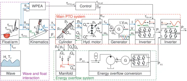
The system is divided into the sub-models seen in Fig. 3. The sub-models are arranged in four main blocks, i.e. Wave Input, Wave and Float Interaction, Main PTO System and Energy Overflow. The Wave Input and Float Arm blocks are fixed, whereas the remaining blocks consist of components, where component sizes and control is to be optimized to minimize losses and maximize power output of the WEC.
G pA pB Fc QBc QAc pB pA τM α QA QB ωG τtot τextτPTO I,V,ωv θarm xc darm
Float/arm Kinematics Cylinder Hyd. motor Generator Inverter
Wave H Ts, P ωarmθarm τPTO τext xc vc Fc QB QA pB pA τM ωG I V ωv ωv Manifold QB QA QEO pB pA QAQB pEO
Energy overflow conversion G Inverter ωv PEO Pout PEO P1 Main PTO system
Energy overflow system Wave and float
interaction WPEA θarm ωarm Control τPTO,ref αref τGn,ref τGn,ref αref
Figure 3: System model for evaluating and optimising PTO performance.
Multiple levels of optimization is performed, see Fig. 4. The WPEA algorithm calcu-lates the time-varying torque τref to maximize the expected energy output of the WEC,
taking into account the PTO efficiency. Hence, an initial efficiency guess is required. Next, the PTO control is tuned and the system is evaluated, and with a new efficiency, the WPEA algorithm is updated. With a converged solution of WPEA and control, the losses of the components are identified. With this knowledge the component sizes and properties are re-adjusted and the loop is performed again.
WPEA controlPTO
System Evaluate PTO OK? control Eff. converg-ed? Sys. perform. conv.? Initial system Y Y Y Update control Update WPEA Manual update system N N N PTO evaluated
Figure 4: Strategy for optimising and evaluating the PTO system.
3. MODELLING
3.1. Wave Model
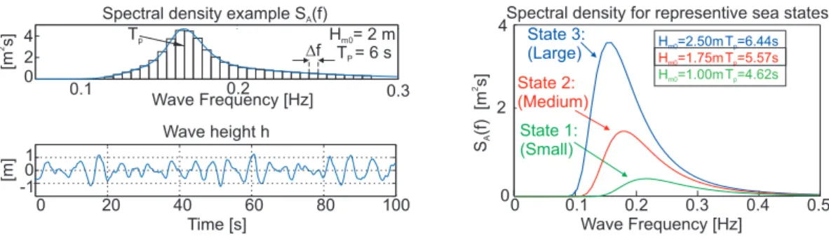
Ocean waves are irregular waves, i.e. waves with varying frequency and amplitude. As a result, irregular waves are described by a wave amplitude spectrum, see Fig. 5. A sea state or spectrum is usually represented by two quantities, the significant wave height Hs and the peak wave period Tp. The significant wave height is the average of
the wave heights of the one-third highest waves, and Tp is the period where the waves
at average are highest. The Pierson-Moskowitz spectrum is utilized [11].
0.1 0.2 0 2 4 Wave Frequency [Hz] [m s] 2 0.3 Df 0 20 40 60 80 100 -1 0 1 Time [s] [m] Tp H = 2 mm0 T = 6 sP Spectral density example S (f)A
Wave height h 0 0.1 0.2 0.3 0 4 S (f)[m s] A 2 0.5 Wave Frequency [Hz]
Spectral density for representive sea states
H =2.50mm0 H =1.75mm0 H =1.00mm0 T =6.44sp T =5.57sp T =4.62sp State 3: (Large) State 2: (Medium) State 1: (Small) 2 0.4
Figure 5: Wave spectra for sea states and an example of a corresponding wave.
From a spectrum, the individual wave components can be extracted as,
ηw,i(t) =
√
2SA(fi)∆fsin(2πfit) [m] (1)
and a time series of an irregular wave, can be generated as a sum of wave components,
ηw(t) = n ∑ i=1 √ 2SA(fi)∆fsin(2πfit+φrand,i) [m] (2)
where φrand,i is a random phase for each component. This is known as the
random-phase method. However, a more random wave which represents sea waves better is obtained by filtering white noise using proper digital filters designed according to the spectra, see [11] for reference. This method is utilized instead to generate time-series of waves.
To evaluate the performance of the PTO, the three sea states shown in Fig. 5 are used, which represents the range of waves in which the WEC should be able to produce power. A wave time series has been generated for each sea state for evaluation of PTO performance.
The following section describes how the wave interacts with the float. 3.2. Wave and Float Interaction
The equation of motion for a float is given as,
Jarm+floatθ¨arm(t) =τwave(t)−τG(t)−τPTO(t) [Nm] (3)
where Jarm+float is the inertia of float and arm, τwave is the torque due to wave-float
interaction, τG is the torque due to gravity and τPTO is the torque applied by the PTO
system to the float arm.
To describe the interaction between wave and float, τwave(t), linear wave theory is
often applied, as it gives an adequate description in the conditions in which a WEC is producing energy, [14]. In linear wave theory simplified fluid dynamics is assumed
in order to apply linear potential theory. Resultantly, the wave-float interaction can be described by superimposing three torques,
τwave(t) =τrad(t) +τArch(t) +τext(t) [Nm] (4)
where τext(t) is the excitation torque an incoming regular wave applies to a float held
fixed, τrad(t) is the radiation toque experienced from oscillating the float in otherwise
water, and τArch is the torque due to the Archimedes force, i.e. buoyancy.
The sum of the three torques gives,
τwave(t) = |−J∞ω˙arm(t)−{zhrad(t)∗ωarm(t})
τrad
+τArch(t) +τext(t) [Nm] (5)
where hrad is the impulse response function from float velocity to torque, describing
the hydrodynamic damping. The impulse response hrad can be viewed as a high order
damping term. The inertia term J∞ represents the ”added mass”, which contains the effect, that when oscillating a float, it will appear to have a greater mass due to the water being displaced along with the float.
The coefficients of Eq.5 are identified by applying the numerical tool WAMIT to the float. WAMIT is a computer program for computing wave loads and motions of structures in waves [12]. WAMIT also outputs a force filter, which can be applied to
ηw(t) to find τext(t).
Inserting Eq.5 into Eq.3 gives the equation of motion for the float, ˙
ωarm=
1
Jarm+float+J∞
(
−kresθarm(t)−hrad(t)∗ωarm(t)+τext(t)−τPTO(t)
)
[ms2 ] (6)
where the sum of gravity and Archimedes term has been linearised around the draft of the float, τres(t) =τArch(t)−τG(t)≈θarm(t)kres. Thus the input to float-arm subsystem
are the torques τext and τPTO, and the output is the angular position and velocity of the
arm. To avoid the convolution term hrad(t)∗ωarm(t), the impulse response has been
fitted with a fifth-order system using Prony’s methods [15].
The power extracted or harvested from a wave Phav is the product of the PTO torque τPTOand arm velocityωarm. Hence,τPTO should be controlled such that harvested energy Ehav is optimised:
Ehav =
∫ ∞
0
τPTO(t)ωarm(t)dt [J] (7)
In general, to maximise Eq.7 the float should be in phase with the exiting wave torque
τext, i.e. the natural frequency of the float and arm should match the incoming wave.
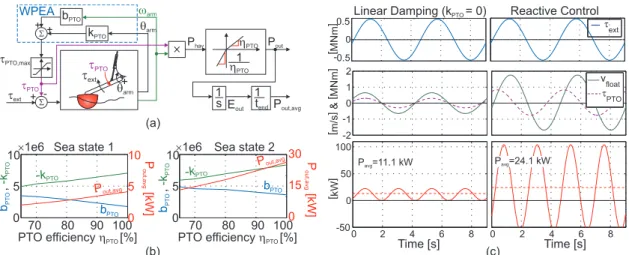
However, as the dominating wave frequency varies, the natural frequency will not match. Consequently, the PTO system is used to move the natural frequency to increase power capture. This is depicted in Fig. 6a, where the reference of the PTO torque is generated by a damping term bPTO and a spring term kPTO:
τPTO,ref=kPTOθarm+bPTOωarm [Nm] (8)
The effect of including the stiffness term is illustrated in Fig. 6c, where a regular wave is applied to the system. In the first case, linear damping is utilized, i.e. kPTO
is zero, and in the second case kPTO is non-zero (Reactive control). When using the
linear damping, the power Phav is always positive. In the second case, the power is
periodically negative, but the average harvested power is twice compared to linear damping. Hence, more power is extracted, but it requires a PTO with four-quadrant operation as reactive power is involved.
The optimal control in regard to power output depends on the PTO efficiency ηPTO,
as the loss associated with the power required to move the natural frequency begins to outweigh the extra harvested power. To find the optimal parameters bPTO and kPTO
as a function of PTO efficiency ηPTO, time-series simulation has been executed for
different efficiencies and sea states, and the values of bPTO and kPTO maximising the
average power Pout,avg have been found. These were found by using a simplex-based
optimisation algorithm. The simulation model is seen in Fig. 6a. Note that also a saturation limit has been added to the PTO torque of 1 MNm, as it has been found to be a reasonable limit in regard to harvested power versus requirements of the PTO. The limit have been found by multiple simulations,where the limit have gradually decreased. The results for the optimal values of kPTO and bPTO for sea state 1 and sea
state 2 is seen in Fig. 6b as a function of efficiency. Also the expected power outputs are shown. bPTO kPTO t ext S S t PTO + -+ q arm w arm + t ext t PTO q arm + Phav (c)
Linear Damping (kPTO= 0) Reactive Control WPEA h PTO h PTO 1 Pout t PTO,max 1 s Eout (a) bPT O , -kPT O ´1e6 P [kW] out,avg bPT O , -kPT O ´1e6
PTO efficiencyhPTO[%] PTO efficiencyhPTO[%]
Sea state 1 Sea state 2
Time [s] Time [s] (b) P [kW] out ,a vg 1 tendPout,avg 70 80 90 100 70 80 90 100 10 5 0 10 5 0 10 5 0 30 15 0 -kPTO -kPTO bPTO bPTO Pout,avg Pout,avg
Figure 6: Power extraction from waves, optimising the WPEA as a function ofηPTO.
3.3. Hydraulic System - Main PTO System
The hydraulic system consist of a closed circuit pump/motor and a cylinder. The output of the hydraulic system is the torque τM for driving the generator, and the cylinder
force Fc acting on the float and arm.
To simplify dynamics, hose losses are neglected, such that the pressure in cylinder and at motor are equal. Power loss associated due to hose loses will be discussed afterwards when evaluating efficiency.
Using the flow continuity equation the following expression is obtained for the sym-metric cylinder, ˙ pB = βe,1 Acxc+V0,1 (−QB−v˙cAc) [bars ] (9) ˙ pA = βe,2 Ac(xc,max−xc) +V0,2 (QA+ ˙vcAc) [bars ] (10)
whereAcis the cylinder area,xc,maxis the maximum stroke of cylinder and the volumes V0,1 and V0,2 are volumes of hoses.
The cylinder force is calculated as, Fc= ∆pAc−Ffric ; Ffric= tanh(avc)|∆pAc|(1−ηc) ; ∆pAcvc >0 tanh(avc)|∆pAc| ( 1 ηc −1 ) ; ∆pAcvc ≤0 [N] (11)
where ∆p=pB−pA. The cylinder frictionFfric is defined such that the cylinder has a
constant efficiency of ηc. The function tanh(avc) is used instead of sign(vc) to avoid
discontinuity, where a adjust the steepness around zero velocity.
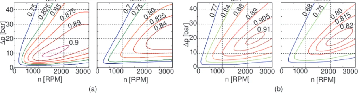
The hydraulic motor is a closed-circuit swash-plate pump. The model is based on measured efficiency plots for different pump sizes. A typical efficiency plot is seen in Fig. 7a for 100% and 50% displacement respectively. Using Schlösser formula [13] for friction and flow loss, the following expression are used for motor torque and flow:
QM,nom(ωM,∆p) =αDωωM−∆pCQ1 [m 3 s ] (12) τM,nom(ωM,∆p) =αDω∆p− ( Cτ1+Cτ2∆p+Cτ3ωM+Cτ4ω2M ) [Nm] (13) The efficiency of the fitted model is seen in Fig. 7b. If the fitted pump is referred to as the nominal size, other motor size is obtained by scaling this model,
QM,new(ωM,∆p) = Dω,new Dω,nom ωrated,new ωrated,nom QM,nom ( ωrated,nom ωrated,new ωM,∆p ) [ms3 ] (14) τM,new(ωM,∆p) = Dω,new Dω,nom τM,nom ( ωrated,nom ωrated,new ωM,∆p ) [Nm] (15) where Dω,new and ωrated,new is the displacement and rated speed of the new motor
respectively. ∆ p [ bar] 0.9 0.89 0.875 0.85 0.825 0.75 0 10 20 30 40 0.84 0.825 0.80 0.75 0.7 0.77 0.84 0.88 0.89 0.905 0.91 0.68 0.75 0.80 0.815 0.82 n [RPM] 1000 2000 3000 n [RPM] 0 0 10 20 30 40 ∆ p [ bar] α=1 α=0.5 1000 2000 3000 0 1000 2000 3000 0 0 1000 2000 3000 n [RPM] n [RPM] (a) (b) α=1 α=0.5
Figure 7: Efficiency plots for a typical swash-plate pump, measurements and model.
To replenish the fluid leaked by the motor and to give the necessary flushing for cooling and filtering, a charge/booster pump is installed. The charge pump is set to maintain a pressure of 17 bar, which is a low but sufficient charge pressure. According to data sheets a rule-of-thumb is to size the charge pump to be 10% of the installed displace-ment. Consequently, to model the required power for flushing, a fixed displacement pump running together with the motor is used:
Pflush =Dω,charge pcharge ωM= 0.1Dω,Mpcharge ωM [W] (16)
Regarding swash-plate dynamics, it is assumed that the swash-plate control is fast enough for controlling the pressure as the pressure reference is dictated by the wave frequency, which is low. Hence swash-plate dynamics is omitted.
3.4. Generator and Inverter - Main PTO System
The generator setup consists of an asynchronous generator and an inverter for grid connection and to enable variable speed control. The input to the generator is the hydraulic motor torque and the output of the power system is the angular velocity of the generator ωM and output power.
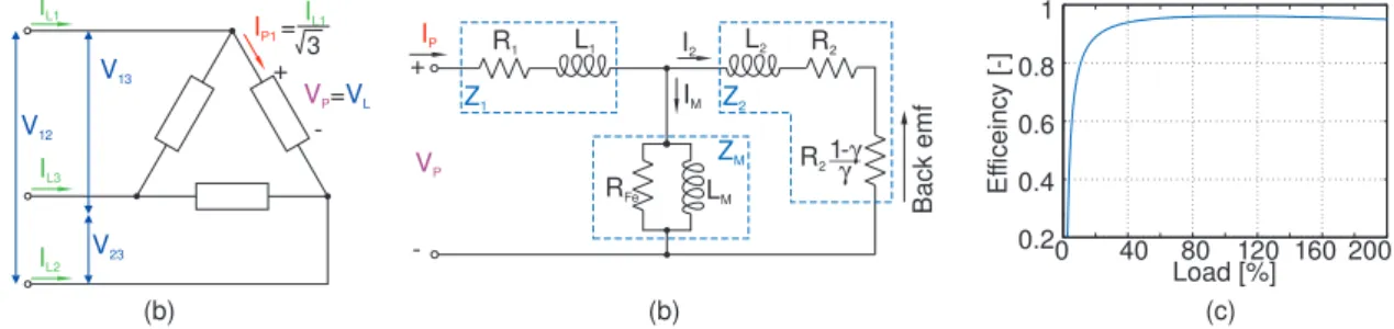
The electrical properties of the generator is modelled in steady state. This assumed to be adequate, as the inverter handles the dynamics. An equivalent circuit for a phase of a three-phase Delta-connected induction motor is seen in Fig. 8b, where γ denotes the motor slip. The slip is defined as,
γ = 1− nppωGn
ωV
[−] (17) wherenppis the number of pole pairs andωVis the frequency of the supply voltage. The
resistorR21−γγ represents the mechanical input to the generator, i.e.τGnωGn=I2R21−γγ,
for reference see e.g. [16].
As the current I2 ≫IM, the generator torque is given as, τGn = 3nppR2 γωV VRMS2 ( R1+R2+ 1−γγR2 )2 + (ωV(L1+L2))2 [Nm] (18) where VRMS is the RMS-value of the line-to-line voltage.
The steady-state phase current IP of the generator is given as: IP= VP |HGn(jωV)| , HGn(jωV) = Vp IP = Z2(s)ZM(s) Z2(s) +ZM(s) +Z1(s) s=jωV (19) where Z1 =R1+L1s, Z2 = Rγ2 +L2s and ZM= RRFeFe+sLsLMM.
The electrical output power of the generator is three times the power per phase:
PGn,out = 3VPIPcos(̸ HGn(jωV)) =
√
3VLILcos(̸ HGn(jωV)) [W] (20)
As hydraulics motors are typically operated in the range of 500-2500 RPM, a 4-poled generator is used, as it operates at 1500 RPM at a voltage frequency of 50 Hz. A nominal model is based on the measurement of an asynchronous high-efficiency 4-pole 55-kW generator, where the parameters of the equivalent circuit has been identified. The model result is seen in Fig. 8c, where the efficiency is plotted as a function of load at 1500 RPM. The torque characteristic as a function of slip produced by the model seen in Fig. 9. Other generator sizes are obtained by scaling the nominal model similar to the methods applied to the hydraulic motor.
The angular velocity of the generator is given by, ˙
ωGn =
1
JGn+JM
(τM−τGn) [s12 ] (21)
where JGn and JM is the inertia of the rotor of the generator and hydraulic motor
respectively.
The torque of the generator is controlled by an inverter. The inverter is modelled with a constant efficiency ηinv of 95%. To control the torque of the generator, the
expressions for finding the appropriate voltage and voltage frequency for the generator is implemented in the inverter, see Fig. 9. The modelled 55 kW generator may be operated at 150% load for two minutes, and may in shorter periods also be operated at 200% load. Consequently, the inverter is limited to run the generator at 200% load.
R2 R2 L2 L1 R1 RFe LM 1-γ γ VP IP I2 + -IL1 IL2 IL3 V12 V23 V13 IP1= + -VP=VL 3 IL1 (b) (b) Back emf IM Z1 Z2 ZM 0 40 80 120 160 200 0.2 0.4 0.6 0.8 1 Load [%] Ef ficeinc y [-] (c) Figure 8: Per phase equivalent circuit for an induction motor.
-0.04 -0.02 0 0.02 0.04 -800 -400 0 400 800 Slip [-] [Nm] τGn,ref γ npp Gn ω 1 -γ ωV= ωV VL≈ ωGn2π 400 V50 Hz VL ωV VL G ωGn τM I ,V ,L Lωv ωV ωGn Inverter PGn,out ηinv ηinv1 Pinv,out Generator τM Generator torque at 1500RPM τGn,ref γ
Figure 9: Torque characteristic of generator and torque control of generator.
3.5. Energy Overflow System
If a float cylinder produces more flow than the hydraulic motor can consume, the pressure builds up in the cylinder until opening the check-valve to the Energy Overflow (EO) system. Due to accumulators the EO system is assumed to be operating at a steady high pressurepEO. As simulating the behaviour of the EO system would require
to simulate all 20 floats, a fixed efficiency is assumed instead for the EO system. A model of a check-valve to connect the cylinder to the EO system is included, which determines the flow QEO entering the EO system. The remaining EO system consist
of a long pipeline to connect overflow from all floats, a fixed displacement motor, a generator and an inverter. The following efficiency ηEO is used for the EO system:
ηEO =ηpipe,avgηM,avgηGn,avgηinv,avg = 0.95·0.90·0.90·0.95 = 0.73 (22)
Hence, if the power delivered to the EO system isPEO,in =pEOQEO, the power delivered
to the grid from the EO system is PEO,out =PEO,inηEO.
3.6. Calculating Efficiencies and Power Losses
To optimize and evaluate the PTO system, power losses and efficiencies of the individ-ual components are calculated. If the instantaneous power in and out of a component are Pin and Pout respectively, the efficiency and losses are calculated as:
Pin,avg = 1 tend ∫ tend 0 Pin(t)dt , Pout,avg = 1 tend ∫ tend 0 Pout(t)dt (23) η= Pin,avg Pout,avg
, Ploss,avg=Pin,avg−Pout,avg (24)
As power transfer in both direction occur, the efficiency does not specify the component efficiency but a resulting efficiency, e.g. a component with a fixed efficiency will show a lower efficiency when reactive power is involved.
4. DESIGN OF PTO
The design of PTO is organized by first taking a brief view on the requirements, combined with an initial sizing of the PTO components. For evaluating the PTO performance, three different control strategies for control of motor and generator are developed and applied. Based on the control strategies and initial sizing, the PTO system is optimised.
4.1. Requirements and Initial Sizing of PTO
The requirements of the PTO system is to be able to produce power at sea states ranging from a significant wave height of about 1 m to 3 m. To design and evaluate the PTO system, the three representative sea states defined in Fig. 5 are utilized.
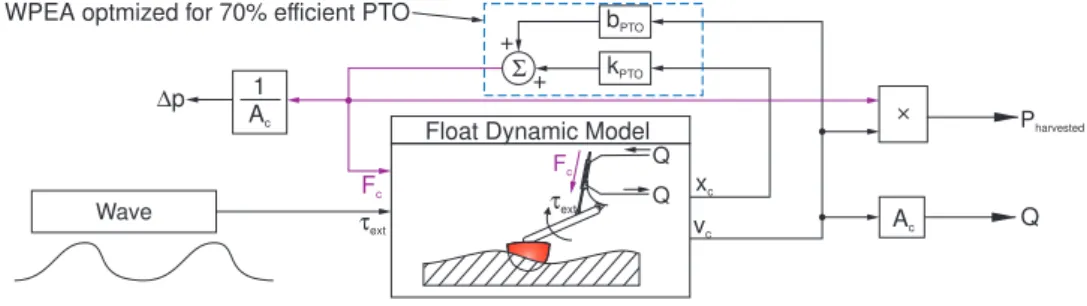
In order to quantify the requirements, simulation of cylinder forces Fc and power
input have been made by applying the three different sea states to the float model, see Fig. 10, where a power extraction algorithm tuned for a PTO with a efficiency of 70% is applied. Roshage float τext xc Pharvested Wave Fc Q Q Float Dynamic Model
vc
bPTO
kPTO
Σ+ + WPEA optmized for 70% efficient PTO
τext Fc 1 Ac ∆p Ac Q
Figure 10: Simulation for estimating requirements of PTO.
The flow and pressure requirements depends on the cylinder size. To minimize flow losses, the pressure should be as high as possible, however, according to the typical pump efficiency data displayed in Fig. 7, the efficiency drops above 300 bar. As a result, the cylinder is designed such that the maximum required force is obtained at a delta pressure of 300 bar. To give a torque of 1 MNm, a cylinder force of 420 kN is required, yielding Ac = 140cm2. The pressure of the EO system is set to 325 bar. The result
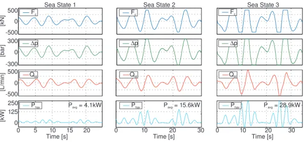
of applying the cylinder area to the simulation is seen in Fig. 11, where the required pressures and flows are seen.
According to Fig. 11 the peak power in sea state 3 is about 250 kW, however having e.g. a 250 kW hydraulic motor and generator producing an average power of 29 kW will lead to very poor efficiencies. As sea state 2 is more frequently occurring, the first iteration of a PTO is based on this sea state. The peak flows are approximately 250 L/min. If the generator is set to run at a fixed speed of 1500 RPM, a 160 cc motor is required.
If the generator is assumed to be able run at 100% overload in shorter periods, the generator matching a hydraulic motor is found as,
τM,max=Dω∆pmax [Nm] (25)
PGn,norm=
1
2τM,max·ωGn,max [W] (26)
28.93 0 5 10 15 20 0 10 20 30 0 10 20 30 -500 500 0 -300 300 0 -500 500 0 250 0 125 [kN] [bar] [L/min] [kW]
Phav Pavg= 4.1kW Phav Pavg= 15.6kW Phav Pavg= 28.9kW
Time [s] Time [s] Time [s]
QM QM QM
∆p ∆p
Fc Fc
Fc
∆p
Sea State 1 Sea State 2 Sea State 3
Figure 11: Power, flow and pressure at different sea states.
displacement of the hydraulics motor in m3/s. The pressure∆p
maxis maximum allowed
pressure, in this case 300 bar.
The generator size matching a 160 cc motor is then a 60 kW unit. If the cylinder produces more flow than the motor can consume, the pressure builds up until opening the check-valve to the Energy Overflow (EO) system.
4.2. PTO Control Strategies
The objectives of the PTO control is to track the cylinder force reference produced by the WPEA algorithm while minimizing power losses. The control inputs are the displacement control α of the hydraulic motor and the generator torqueτGn.
Three control strategies are tested:
1) Fixed speed of generator according to sea state and force control using α
2) Slowly varying generator speed according to average peak flow requirement. 3) Generator speed is controlled to keep motor displacement α at maximum. A comparison of the three control strategies is shown in Fig. 12. In the first strategy the generator is running at 1500 RPM, as a result, the motor is at part stroke most of the time. In strategy 2 the engine speed is varied according to the average required flow, which leads to the motor being closer to full stroke. In strategy 3 the generator speed is continues controlled to get the motor to 95% stroke, however this requires the generator speed to oscillate together with the wave. To avoid using to much electrical power to accelerate the generator inertia, the generator is not allowed to operate in motor mode above e.g. 1000 RPM.
4.3. Evaluation and Optimization of PTO
The initial PTO design is evaluated for each sea state using the three described control strategies. The results seen in Tab. 1, Tab. 2 and Tab. 3, where PL and η denotes
average power loss [kW] and efficiency [%] respectively, and the columns Pin andPout
are the average harvested power and power output of the system in [kW]. The overall efficiency and power output is best for control method three. It overall gives a 2 kW higher output. Control strategy 1 and 2 giv approximately the same power output,
are
Control Strategy 1 Control Strategy 2 Control Strategy 3 Displacement contr ol [-] α Gener at or speed [RPM] ωGn
Time [s] Time [s] Time [s]
Figure 12: Comparison of the three control strategies.
however, strategy 2 has a better efficiency, so the required cooling would be lower. From the tables it seen that generally, the hydraulic motor is dropping below 80% efficiency in sea state 1 and 2. Also, the generator efficiency is dropping low in sea state 1.
Table 1: Initial system with control strategy 1
SS Cylinder Motor Flush Generator Inverter EO Total
PL η PL η Pflush PL η PL η PL Pin Pout η
1 0.31 94.4 1.52 69.8 0.34 0.80 74.8 0.27 88.7 0.00 5.48 2.09 38.2 2 1.32 94.3 5.14 74.3 0.68 1.74 87.7 1.10 91.2 0.29 23.2 12.3 52.9 3 2.39 94.6 7.26 78.5 0.68 2.21 91.5 1.73 92.7 1.58 44.0 27.1 61.6
Table 2: Initial system with control strategy 2
SS Cylinder Motor Flush Generator Inverter EO Total
PL η PL η Pflush PL η PL η PL Pin Pout η
1 0.34 94.3 1.53 72.1 0.34 0.80 77.9 0.29 89.6 0.00 5.97 2.52 42.2 2 1.20 94.4 3.84 78.8 0.43 1.27 90.8 0.95 92.5 0.34 21.4 12.8 59.7 3 2.25 94.6 6.12 80.3 0.46 1.78 92.7 1.54 93.2 1.74 41.9 27.0 64.4
Table 3: Initial system with control strategy 3
SS Cylinder Motor Flush Generator Inverter EO Total
PL η PL η Pflush PL η PL η PL Pin Pout η
1 0.37 94.2 1.42 75.8 0.30 0.75 82.0 0.27 92.1 0.00 6.39 3.13 49.0 2 1.31 94.3 3.75 81.3 0.39 1.24 92.2 0.96 93.4 0.27 23.2 14.6 63.1 3 2.35 94.6 5.89 82.8 0.42 1.79 93.6 1.60 93.9 1.44 43.8 29.3 66.9 By optimising on the simulation model, it has been found that to have good efficiencies at sea state 1 and 2, it is best to utilize a smaller hydraulic motor and instead increase the speed in high power periods, e.g. up to 2500 RPM. After optimising control and components, the values in Tab. 4 have been identified.
Table 4: Optimized system parameters.
Cylinder Area Motor size Generator size Maximum speed
140 cm2 80 cm3 45 kW 2500 RPM
4.4. Optimized Solution
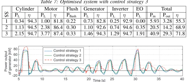
The results for the three control strategies applied to the optimised solution are seen in Tab. 5, Tab. 6 and Tab. 7. Compared to the previous solution, the harvested power
have been reduced with 2-5 kW, however the output power remains unchanged, which gives a rise in efficiency. The average efficiency improvement is 5%. The reduction in harvested power is due to the main PTO system more often becoming saturated, e.g. the flow from the cylinder cannot be consumed by the motor, leading to the pressure rising topEO. As a results, the system cannot track the optimal cylinder force trajectory.
Comparing the results of the three control strategies, strategy 1 and 2 outputs the same amount of power, but less is harvested in strategy 2, giving it a better efficiency score. Strategy 2 harvest less power, as the generator speed is too low in periods. To improve the control, the controller must be improved in predicting when to increase the generator speed. Control strategy 3 shows the best results, harvesting power as control strategy 1 while reducing losses. Also this strategy is able to maintain a motor efficiency above 80% in all sea states.
One of the reasons for the relative good efficiency of strategy 3 is, that the generator power is mostly positive. This is seen in Fig. 13, where the generator power is compared for the three strategies. When the system requires reactive power this is actually taken from the kinetic energy saved in the inertia of motor and generator when the generator speed is reduced. In the two other strategies, the reactive power is drawn from the inverter,
Table 5: Optimised system with control strategy 1
SS Cylinder Motor Flush Generator Inverter EO Total
PL η PL η Pflush PL η PL η PL Pin Pout η
1 0.20 94.7 0.79 77.3 0.17 0.58 76.8 0.17 91.3 0.00 3.83 1.77 46.2 2 1.12 94.5 3.18 80.9 0.45 1.58 87.8 0.88 92.3 0.47 20.2 12.1 60.0 3 2.19 94.7 4.78 83.5 0.50 1.99 91.6 1.47 93.2 2.21 41.2 27.4 66.6
Table 6: Optimised system with control strategy 2
SS Cylinder Motor Flush Generator Inverter EO Total
PL η PL η Pflush PL η PL η PL Pin Pout η
1 0.30 94.4 1.18 76.5 0.28 0.86 75.9 0.25 90.6 0.00 5.45 2.45 44.9 2 1.04 94.5 2.57 83.4 0.35 1.22 90.3 0.77 93.2 0.47 18.9 12.1 64.0 3 2.05 94.7 3.92 85.0 0.37 1.52 93.0 1.27 93.8 2.32 38.8 26.7 68.9
Table 7: Optimised system with control strategy 3
SS Cylinder Motor Flush Generator Inverter EO Total
PL η PL η Pflush PL η PL η PL Pin Pout η 1 0.34 94.3 1.00 81.8 0.22 0.73 82.8 0.25 92.9 0.00 5.93 3.28 55.3 2 1.13 94.5 2.38 86.4 0.30 1.10 92.6 0.74 94.6 0.35 20.5 14.2 68.9 3 2.15 94.7 3.77 87.4 0.33 1.46 94.3 1.29 94.7 1.91 40.9 29.3 71.8 5 10 15 20 25 30 35 -20 0 20 40 60 80 40 Time [s] Control strategy 1 Control strategy 2 Control strategy 3 Poweroutput ofgenerator[kW]
Figure 13: Power output of the generator for the three control strategies.
5. DISCUSSION
Based on the modelled system, the best efficiency achievable of the investigated PTO system is between 55% and 72% in the production range of the wave energy converter. These results are obtained using control strategy 3, see the summarized results in Tab.8. However, control strategy 3 requires the motor and generator to speed up and down according to the float velocity, e.g. from low to high speed two times per wave period. Hence, lifetime of the components may be reduced by this scheme. Consequently, an evaluation of components lifetime should be evaluated before using this control scheme. Nevertheless, control strategy 3 is good for showing the best achievable efficiency with off-the-shelf components.
Table 8: Optimised system performance summary.
SS Control 1 Control 2 Control 3
Pin Pout η Pin Pout η Pin Pout η
1 3.83 1.77 46.2 5.45 2.45 44.9 5.93 3.28 55.3
2 20.2 12.1 60.0 18.9 12.1 64.0 20.5 14.2 68.9
3 41.2 27.4 66.6 38.8 26.7 68.9 40.9 29.3 71.8
The output power of control strategy 1 and 2 is in average 2 kW lower, however these solutions would be easy implementable. As such, control strategy 2 is preferred, as the speed of the motor and generator are reduced during low power periods, e.g. wear and tear is reduced. Regarding generator efficiency, when operating at low speeds as in sea state 1, the generator shows a poor efficiency. This might be raised to about 90% by reducing the magnetizing current, which gives the losses. For same reason, a permanent magnet generator will show better result at sea state 1, but it will not give a significant improvement at sea state 2 and 3.
To assess the accuracy of the results, an overview of the model properties is shown in Tab. 9, along with future improvements. If the transient behaviour was included for the generator, features as reducing the magnetizing current could be evaluated. The remaining features to be added represents additional losses. Hence it would be reasonable to subtract 3-5% from the results.
Table 9: Optimised system with control strategy 1
Cylinder Motor Generator Inverter EO
Included Pressure dynam-ics, hose vol-umes, const. eff.
Friction, flow losses, power for flushing. Mechanical dynamics, steady state electrical model. Const. efficiency, electrical model of generator ctrl. Constant efficiency.
Add Hose loses, cyl. friction model.
Power for stroke control. Electrical dynamics. Efficiency as a function of load. Model EO with 20 floats
To improve efficiency in the future, the swash-plate motor could be replaced with upcoming components like digital displacement motors [17], [18], which are charac-terized by having excellent part load efficiency. Also, the current solution relies on being a multiple absorber system to provide power smoothing. To change the concept to include more smoothing would be advantageous, also to reduce component sizes. Finally, PTO systems characterized by having hydraulic motors for e.g. 2 or 4 floats on a common shaft to power a larger generator have also been investigated during this research. This will increase the generator efficiency, but only control strategy 1 would be applicable. Hence, the motor efficiency drops below 80%, ie. this system setup will not improve the efficiency.
6. CONCLUSION
By optimizing the proposed PTO system for a multiple point absorber system, the best achievable efficiency with conventional components is in the range from 52% to 68% under the different wave conditions at which a wave energy converter is producing power. This emphasizes the need for new component types like digital-displacement motors, or entirely new PTO concepts in order to utilize wave energy from point absorbers. New PTO concepts are therefor currently under investigation.
REFERENCES
[1] A. Muetze and J.G. Vining. Ocean wave energy conversion - a survey. In Industry Applications Conference, 2006.
[2] B. Drew, A. Plummer and M.N. Sahinkaya. A review of wave energy converter technology. Proceedings of the Institution of Mechanical Engineers, Part A: Journal of Power and Energy, 223 (8), 2009.
[3] J Cruz. Ocean Wave Energy: Current Status and Future Perspectives, 2008, Green Energy and Technology Series, ISBN:978-3-540-74894-6.
[4] S.H. Salter, J.R.M. Taylor and N.J. Caldwell. Power Conversion Mechanisms for Wave Energy. Proceedings of the Institution of Mechanical Engineers, Part M: Journal of Engineering for the Maritime Environment, 2002.
[5] J. Falnes. Optimum Control of Oscillation of Wave-Energy Converters. Interna-tional Journal of Offshore and Polar Engineering, vol. 12 2002.
[6] E. Wood. Power generation systems in buoyant structures. US-patent: US4158780, 1979.
[7] A.F. de O. Falcao. Modelling and control of oscillating-body wave energy convert-ers with hydraulic power take-off. Ocean Engineering, vol. 35, 2008.
[8] A. Babarit,M. Guglielmi and A.H. Clement. Declutching control of a wave energy converter. Journal of Ocean Engineering, vol. 36, 2009.
[9] L. Marquis, M. Kramer and P. Frigaard. First Power Production figures from the Wave Star Roshage Wave Energy Converter. 3rd International Conference and Exhibition on Ocean Energy, 2010.
[10] Wave Star A/S. http://www.wavestarenergy.com/
[11] M.J. Ketabdari and A. Ranginkaman. Simulation of Random Irregular Sea Waves for Numerical and Physical Models Using Digital Filters. Transaction B: Mechanical Engineering Vol. 16, No. 3, 2009.
[12] http://www.wamit.com/
[13] K. Huhtala, J. Vilenius, A. Raneda and T. Virvalo. Energy losses of a tele-operated skid steering mobile machine. Power transmission and motion control, 2002. [14] J.Falness. Ocean Waves and Oscillating Systems. ISBN: 0-521-78211-2
[15] G. De Backer. Hydrodynamic Design Optimization of Wave Energy Converters Consisting of Heaving Point Absorbers. Ph.D. thesis, 2009.
[16] A. Hughes. Electrical motor and drives. Third Edition, 2006, ISBN:0-7506-4718-3 [17] G.S. Payne,U.B.P. Stein, M. Ehsan, N.J. Caldwell and W H.S. Rampen. Potential of Digital Displacement Hydraulics for Wave Energy Conversion. In proc. of the 6th European Wave and Tidal Energy Conference, Glasgow, UK, 2005.
[18] M. Ehsan, W.H.S. Rampen and J.R.M Taylor. Simulation and Dynamic Response of Computer Controlled Digital Hydraulic Pump/Motor System Used in Wave Energy Power Conversion. In proc. 2nd European Wave Power Conference, Lisbon, 1995.
![Figure 1: Point absorber type WECs and the Wavestar 600 kW WEC [10].](https://thumb-us.123doks.com/thumbv2/123dok_us/927058.2620094/2.892.145.760.102.284/figure-point-absorber-type-wecs-wavestar-kw-wec.webp)