Distributed Data Deduplication
Xu Chu
University of WaterlooIhab F. Ilyas
University of WaterlooParaschos Koutris
University of Wisconsin-MadisonABSTRACT
Data deduplication refers to the process of identifying tuples in a relation that refer to the same real world entity. The complexity of the problem is inherently quadratic with re-spect to the number of tuples, since a similarity value must be computed for every pair of tuples. In order to avoid com-paring tuple pairs that are obviously non-duplicates, match-ing algorithms use blockmatch-ing techniques that divide the tuples into blocks and compare only tuples within the same block. However, even with the use of blocking, data deduplication remains a costly problem for large datasets. In this pa-per, we show how to further speed up data deduplication by leveraging parallelism in a shared-nothing computing envi-ronment. Our main contribution is a distribution strategy, calledDis-Dedup, that minimizes the maximum workload across all worker nodes and provides strong theoretical guar-antees. We demonstrate the effectiveness of our proposed strategy by performing extensive experiments on both syn-thetic datasets with varying block size distributions, as well as real world datasets.
1.
INTRODUCTION
Data deduplication, also known as record linkage, or en-tity resolution, refers to the process of identifying tuples in a relation that refer to the same real world entity. Data dedu-plication is a pervasive problem, and is extremely important for data quality and data integration [11]. For example, find-ing duplicate customers in enterprise databases is essential in almost all levels of business. In our collaboration with Thomson Reuters, we observed that a data deduplication project takes 3-6 months to complete, mainly due to the scale and variety of data sources.
Data deduplication techniques usually require computing a similarity score of each tuple pair. For a dataset withn
tuples, na¨ıvely comparing every tuple pair requires O(n2) comparisons, a prohibitive cost when n is large. A com-monly used technique to avoid the quadratic complexity is blocking [3, 5, 14], which avoids comparing tuple pairs that
are obviously not duplicates. Blocking methods first parti-tion all records into blocks and then only records within the same block are compared. A simple way to perform block-ing is to scan all records and compute a hash value for each record based on a subset of its attributes, commonly referred to asblocking key attributes. The computed hash values are calledblocking key values. Records with the same blocking key values are grouped into the same block. For example, blocking key attributes can be the zipcode, or the first three characters of the last name. Since one blocking function might miss placing duplicate tuples in the same block, thus resulting in a false negative (for example, zipcode can be wrong or obsolete), multiple blocking functions [11], and overlapping blocks [14, 15], are often employed to reduce the number of false negatives.
Despite the use of blocking techniques, data deduplica-tion remains a costly process that can take hours to days to finish for real world datasets on a single machine [22]. Most of the previous work on data deduplication is situated in a centralized setting [3, 5, 6, 14], and does not leverage the capabilities of a distributed environment to scale out com-putation; hence, it does not scale to large distributed data. Big data often resides on a cluster of machines intercon-nected by a fast network, commonly referred to as a “data lake”. Therefore, it is natural to leverage this scale-out envi-ronment to develop efficient data distribution strategies that parallelize data deduplication. Multiple challenges need to be addressed to achieve this goal. First, unlike centralized settings, where the dominating cost is almost always com-puting the similarity scores of all tuple pairs, multiple fac-tors contribute to the elapsed time in a distributed comput-ing environment, includcomput-ing network transfer time, local disk I/O time, and CPU time for pair-wise comparisons. These costs also vary across different deployments. Second, as it is typical in a distributed setting, any algorithm has to be aware of data skew, and achieve load-balancing [4, 9]. Every machine must perform a roughly equal amount of work in order to avoid situations where some machines take much longer than others to finish, a scenario that greatly affects the overall running time. We show the effect of data skew when we discuss distribution strategies in Section 4. Third, the distribution strategy must be able to handle effectively multiple blocking functions; as we show in this paper, the use of multiple blocking functions impacts the number of times each tuple is sent across nodes, and also induces re-dundant comparisons when a tuple pair belongs to the same block according to multiple blocking functions.
data deduplication. However, it only optimizes for compu-tation cost, and requires a large memory footprint to keep the necessary statistics for its distribution strategy, thus lim-iting its performance and applicability, as our experiments show in Section 6. The problem of data deduplication is also closely related to distributed join computation, which will be discussed in detail in Section 7. However, parallel join al-gorithms are not directly applicable to our setting: (1) most of the work on parallel join processing [25, 2] is for two-table joins, so the techniques are not directly applicable to self-join without wasting almost half of the available workers, as shown in Section 3; (2) even with an efficient self-join implementation, applying it to every block directly without considering the block sizes yields a sub-optimal strategy, as shown in Section 4.2; and (3) to the best of our knowledge, there is no existing work on processing a disjunction of join queries, a problem we have to tackle in dealing with multiple blocking functions.
In this paper, we propose a distribution strategy with op-timality guarantees for distributed data deduplication in a shared-nothing environment. Our proposed strategy aims at minimizing elapsed time by minimizing the maximum cost across all machines. It is important to note that while block-ing affects the quality of results (by introducblock-ing false nega-tives), we do not introduce a new blocking criteria, rather we show how to execute a given set of blocking functions in a distributed environment. In other words, our technique does not change the quality but tackles the performance of the deduplication process. We make the following contribu-tions:
• We introduce a cost model that consists of the maxi-mum number of input tuples any machine receives (X), and the maximum number of tuple pair comparisons any machine performs (Y) (Section 2). We provide a lower bound analysis forX andY that is independent of the actual dominating cost in a cluster.
• We propose a distribution strategy for distributing the workload of comparing tuples in a single block (Sec-tion 3). BothXandY of our strategy are guaranteed to be within a small constant factor from the lower boundXlow andYlow.
• We proposeDis-Dedup for distributing a set of blocks produced by a single blocking function. The X and
Y of Dis-Dedup are both within a small constant fac-tor fromXlow andYlow, regardless of block-size skew
(Section 4). Dis-Dedup also handles multiple blocking functions effectively, and avoids producing the same tuple pair more than once even if that tuple pair is in the same block according to multiple blocking func-tions (Section 5).
We perform extensive experiments on synthetic datasets with varying block-size skew, and on real datasets. Our experiments demonstrate the effectiveness of our proposed distribution strategy (Section 6).
2.
PROBLEM DEFINITION AND
SOLUTION OVERVIEW
In this section, we present the parallel computation model we will use in this paper. We formally introduce the problem definition, and provide an overview of our solution.
2.1
Parallel Computation Model
We focus on scale-out environments, where data is usually stored in what is called adata lake. Such an environment usually adopts a shared-nothing architecture, where multi-ple machines, or nodes, communicate via a high-speed inter-connect network, and each node has its own private memory and disk. In every node there are typically multiple virtual processors running together, so as to take advantage of the multiple CPUs and disks available on each machine and thus increase parallelism. These virtual processors that run in parallel are calledworkers in this paper.
In a shared-nothing system, there is usually a trade-off be-tween thecommunication costand thecomputation cost[30]. For a particular data processing task, it is often hard to pre-dict which type of cost is dominating, let alone constructing an objective function that combines these two costs. In ad-dition, the influence of each cost on the running time is dependent on many parameters of the cluster configuration. For example, there are more than 250 parameters that are tunable in a Hadoop cluster1. In this paper, we follow a sim-ilar strategy used in parallel join processing [25], and seek to minimize both costs simultaneously.
Since all workers are running in parallel, to minimize the overall elapsed time, we focus on minimizing the largest cost across all workers. For workeri, letXi be the
communica-tion cost, and Yi be the computation cost. Assume that
there arekworkers available. We defineX (resp. Y) to be the maximumXi(resp. Yi) at any worker:
X = max
i∈[1,k]Xi (1)
Y = max
i∈[1,k]Yi (2)
A typical example of a parallel shared-nothing system is MapReduce [8]. MapReduce has two types of workers: the mapper and thereducer. A mapper takes a key-value pair, and generates a list of key-value pairs; while a reducer takes a key associated with a list of values, and generates another list of key-value pairs. The input keys of the reducers are the output keys of the mappers. Users have the option of imple-menting a customizedpartitioner. Partitioners decide which key-value pairs are sent to which reducers, based on the key. MapReduce balances the load between mappers very well, however, it is the programmers’ responsibility to ensure that the workload across different reducers is balanced.
2.2
Formal Problem Definition
We are given a datasetI withntuples, sblocking func-tionsh1, . . . , hs, and a tuple-pair similarity functionf.
Ev-ery blocking function h ∈ {h1, . . . , hs} is applied to every
tuple t, and returns a blocking key value h(t). A block-ing function h divides alln tuples into a set of m blocks {B1, B2, . . . , Bm}, where tuples in the same block have the
same blocking key value. Tuple pairs in the same block are compared usingfto obtain a similarity score. Based on the similarity scores, a clustering algorithm is then applied to group tuples together. We emphasize that the goal of this paper is to perform data deduplication efficiently in parallel given a set of predefined blocking functions and the simi-larity function, which is an orthogonal to the problem of
1
designing good blocking strategies [28, 32], or to the prob-lem of designing good similarity functions [23] in order to improve data deduplication quality.
We perform data deduplication using the computational model described in Section 2.1. In this case,Xi represents
the number of tuples that Workerireceives; andYi
repre-sents the number of tuple pair comparisons that Worker i
performs. We aim at designing a distribution strategy that minimizes (a) the maximum number of tuples any worker receives, namely, X, and (b) the maximum number of tu-ple pair comparisons any worker performs, namely, Y, at the same time. This may not be possible for a given data deduplication task, but we show that we can always achieve optimality for bothXandY within constant factors. Hence, our algorithm will perform optimally independent of how the runtime is as a function ofX andY.
Example 1. Consider a scenario where a single blocking
function produces few large blocks and many smaller blocks. To keep the example simple, suppose that a blocking function partitions a relation ofn= 100 tuples into5 blocks of size 10and25blocks of size2. The total number of comparisons
W in this case isW = 5· 10 2 + 25· 2 2 = 250 comparisons. Assume k = 10 workers. Consider first a strategy that sends all tuples to every worker. In this case, Xi = 100
for every worker i, which results in X = 100 according to Equation(1). We then assignYi= Wk = 25comparisons to
workeri (for example by assigning to worker ituple pairs numbered[(i−1)W
k, i W
k]). Therefore,Y = 25according to
Equation(2).This strategy achieves the optimalY, sinceW
is evenly distributed to all workers. However, it has a poor
X, since every tuple is replicated10times.
Consider a second strategy that assigns one block entirely to one worker. For example, we could assign each of the5 blocks of size10 to the first 5 workers, and to each of the remaining 5 workers we assign 5 blocks of size 2. In this case, X = 10, since each worker receives exactly the same number of tuples; moreover, each tuple is replicated exactly once. However, even though the input is evenly distributed across workers, the number of comparisons is not. Indeed, the first 5 workers perform 102
= 45 comparisons, while the last 5 workers perform only 5· 22
= 5 comparisons. Therefore,Y = 45 according to Equation (2).
The above example demonstrates that the distribution strategy has significant impact on both X and Y, even in the case of a single blocking function. In the next three sec-tions, we show how we can construct a distribution strategy that achieves an optimal behavior for bothXandY for any distribution of block sizes, and outperforms in practice any alternative strategies.
2.3
Solution Overview
Consider a blocking function h that produces m blocks
B1, B2, . . . , Bm. A distribution strategy would have to
as-sign, for every block Bi a subset of the k workers of size
ki≤kto handleBi.
A straightforward strategy assigns one block entirely to one worker, i.e.,ki= 1,∀i∈[1, m], hence, parallelism
hap-pens only across blocks. Another straightforward strategy uses all the available workers to handle every block, i.e.,
ki =k,∀i∈ [1, m], hence, parallelism is maximized for
ev-ery block, and uses an existing parallel join algorithms [2,
25] to handle every block. However, both strategies are not optimal, as we will show in Section 4.2.
In light of these two straightforward strategies, we first study how to distribute the workload of one block Bi to
ki workers to minimize X and Y (Section 3). Given the
distribution strategy for a single block, we then show how to assign workers to blocksB1, . . . , Bmgenerated by a single
blocking functionh, so as to minimize bothX andY across all blocks (Section 4). Given the distribution strategy for a single blocking functionh, we will finally present how to assign workers given multiple blocking functionsh1, . . . , hs,
so that the overallX andY are minimized (Section 5). For simplicity, we describe our distribution strategy in MapReduce terms, however, the proposed technique can be implemented in any shared-nothing parallel system, and achieves the same guarantees for bothX andY.
3.
SINGLE BLOCK DEDUPLICATION
In this section, we study the problem of data dedupli-cation for tuples in a single block that is produced by one blocking function; in other words, we need to compare every tuple with every other tuple in the block. The distribution strategy presented in this section will serve as a building block when discussing distribution strategies in Sections 4 and 5. Assume that there aren tuples in the block, andk
available reducers to compute the pair-wise similarities.
3.1
Lower Bounds
We first analyze the lower bounds Xlow and Ylow forX
and Y, respectively. The lower bounds are necessary to reason about the optimality of our distribution strategies.
Theorem 1. For any distribution strategy that performs
data deduplication on a block of size n using k reducers, the maximum input is X > Xlow = √n
k and the maximum
number of comparisons isY ≥Ylow= n(n
−1) 2k .
Proof. To show the lower bound on the number of com-parisons Y, observe that the total amount of comparisons required is n2= n(n2−1). Since there arekavailable reduc-ers, there must exist at least one reducerjwithYj≥ n(n
−1) 2k .
For the lower bound on the input, suppose for the sake of contradiction that the maximum input isn0≤n/√k. Then, each reducer will perform at most n20
comparisons, which means that the total number of comparisons will be at most
k n20
=n(n−√k)/2< n(n−1)/2, a contradiction (since the comparisons must be at least n2).
As we show in Section 3.2, our algorithm matches the lower boundYlow, but notXlow. The problem of designing
a strategy that matches Xlow is tightly related to an
ex-tensively studied problem in combinatorics called covering design[29]. A (n, `, t)-covering design is a familyF of sub-sets of size` from the universe{1, . . . , n}, such that every subset of sizetfrom the universe is a subset of a set inF. The task in hand is to compute the minimum sizeC(n, `, t) of such a family. To see the connection with our distribu-tion problem, consider a (n, X,2)-covering designF of size
k. Then, we can assign to each of thekreducers a set from the family (that will be of sizeX); but now, we can perform every comparison in some reducer, since the covering design guarantees that every subset of size 2 (i.e., every pair) will be
(a)R×S join (b) Self-join
Figure 1: Reducer arrangement. (The number in
the upper left corner of each cell is the reducer id.)
in some set (i.e., in some reducer). Thus, designing a strat-egy that achievesXlowmeans finding a (n, Xlow,2)-covering
design, such thatC(n, Xlow,2)≤k.
The lower bound forX presented in Theorem 1 is called the Sch¨onheim bound [29], but the only constructions that match it are explicit constructions for fixed values ofn, `. There exists a large literature of such constructions [13], and it is an open problem to find tight upper and lower bounds. Hence, instead of looking for an optimal solution, our algorithm provides a constant-factor approximation of the lower bound.
3.2
Triangle Distribution Strategy
We present here a distribution strategy, called triangle distribution strategy, which guarantees with high probability a small constant-factor approximation of the lower bounds. The name of the distribution strategy comes from the fact that we arrange thekreducers in a triangle whose two sides have sizel(thusk=l(l+1)/2 for some integerl). To explain why we organize the reducers in such a fashion, consider the scenario studied in [2, 4] where we compute the cartesian productR×S of two relations of sizen: in this case, the reducers are organized in a √k×√k square, as shown in Figure 1(a) fork = 36. Each tuple from R is sent to the reducers of a random row, and each tuple fromS is sent to all the reducers of a random column; the reducer function then computes all pairs it receives. However, if we apply this idea directly to a self-join (whereR =S), the comparison of each pair would be repeated twice, since if a tuple pair ends up together in the reducer (i, j), it will also be in the reducer (j, i). For example, in Figure 1(a) tuplet1is sent to all reducers in row 2 and column 2, and tuplet2 is sent to all reducers in row 4 and column 4. Therefore, the joining of
t1andt2is duplicated at reducers (2,4) and (4,2). Because of the symmetry, the lower left half of the reducers in the square are doing redundant work. Arranging the reducers in a triangle circumvents this problem and allows us to use all available reducers.
Figure 1(b) gives an example of such an arrangement for
k= 21 reducers withl = 6. Every reducer is identified by a two dimensional index (p, q), where p is the row index, and q is the column index, and 1 ≤ p ≤ q ≤ l. Each reducer (p, q) has a unique reducer ID, which is calculated as (2l−p+ 2)(p−1)/2 + (q−p+ 1). For example, Reducer (2,4) marked purple in Figure 1(b) is Reducer 9.
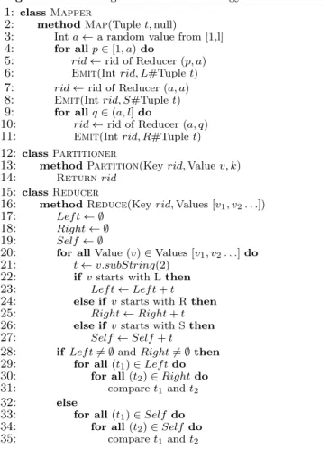
Algorithm 1 describes the distribution strategy given the arrangement for thekreducers. For any tuplet, the mapper randomly chooses an integer a, called an anchor, between [1, l], and distributestto all reducers whose row or column
Algorithm 1Triangle distribution strategy
1: classMapper
2: methodMap(Tuplet,null)
3: Inta←a random value from [1,l]
4: for allp∈[1, a)do
5: rid←rid of Reducer (p, a)
6: Emit(Intrid, L#Tuplet)
7: rid←rid of Reducer (a, a)
8: Emit(Intrid, S#Tuplet)
9: for allq∈(a, l]do
10: rid←rid of Reducer (a, q)
11: Emit(Intrid, R#Tuplet)
12: classPartitioner
13: methodPartition(Keyrid,Valuev, k)
14: Returnrid
15: classReducer
16: methodReduce(Keyrid,Values [v1, v2. . .])
17: Lef t← ∅
18: Right← ∅
19: Self ← ∅
20: for allValue (v)∈Values [v1, v2. . .]do
21: t←v.subString(2)
22: if vstarts with Lthen
23: Lef t←Lef t+t
24: else if vstarts with Rthen
25: Right←Right+t
26: else if vstarts with Sthen
27: Self ←Self+t
28: if Lef t6=∅andRight6=∅then
29: for all(t1)∈Lef tdo
30: for all(t2)∈Rightdo
31: comparet1andt2 32: else
33: for all(t1)∈Self do
34: for all(t2)∈Self do
35: comparet1andt2
index =a (Lines 3-11). By replicating each tuple l times, we can ensure that for every tuple pair, there exists at least one reducer that receives both tuples. In fact, if two tuples have different anchor points, there is exactly one reducer that receives both tuples; while if two tuples have the same anchor pointa, both tuples will be replicated on the same set of reducers, but we only compare the tuple pair on reducer (a, a). The key of the key-value pair of the mapper output is the reducer id, and the value of the key-value pair of the mapper output is the tuple augmented with a flagL, SorR
to avoid comparing tuple pairs that have the same anchor pointsain reducers other than (a, a). Within each reducer, tuples with flag L are compared with tuples with flag R
(Lines 28-31), and tuples with flag S are compared only with each other (Lines 33-35).
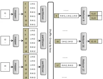
Example 2. Figure 2 gives an example for three tuples
t1, t2, t3given the arrangement of the reducers in Figure 1(b). Suppose that tuple t1 has anchor point a = 2, and tuples
t2, t3have the same anchor pointa= 4. The mapping func-tion takes t1 and generates the key-value pairs (2, L#t1), (7, S#t1),(8, R#t1),(9, R#t1),(10, R#t1),(11, R#t1). Note the different tags L, S, R for different key-value pairs. Re-ducer 9 receives a list of valuesR#t1, L#t2, L#t3associated with key9, and compares tuples marked with R with tuples marked withL, but not tuples marked with the same tag. Re-ducer 16 receives a list of valuesS#t2, S#t3, and performs comparisons among all tuples marked with S.
Figure 2: Single block distribution example using three tuples, given reducers in Figure 1(b)
Theorem 2. The distribution of Algorithm 1 achieves with high probability2maximum inputX ≤(1+o(1))√2X
lowand
maximum number of comparisonsY ≤(1 +o(1))Ylow.
We present the detailed proof in Appendix A, and we provide the intuition here. Fix a reduceri= (p, q). Ifp6=q, the reducer will receive in expectationn/ltuples with flag
L(the ones with anchorp) andn/l tuples with flagR (the ones with anchorR), therefore in expectationXi= 2n/land
Yi=n2/l2. Ifp=q, the reducer will receive in expectation
n/l tuples with flag S, therefore in expectation Xi = n/l
and Yi = n2/2l2. We can show that the Xi and Yi will
also be concentrated around the expectation, and sincek=
l(l+ 1)/2, we haveX≈ √ 2n √ k andY ≈ n2 2k. ComparingX, Y
with the lower bounds in Theorem 1, we have Theorem 2. What happens if the k reducers cannot be arranged in a triangle? Following the same idea that applies when k
reducers cannot be arranged in a square for anR×Sjoin [7], we choose the largest possible integer l0, such that l0(l0+ 1)/2≤k. We havel0(l0+ 1)/2 =k0 ≤k and (l0+ 1)(l0+ 2)/2> k. Since both (l0+ 1)(l0+ 2)/2 andk are integers, we have (l0+ 1)(l0+ 2)/2−1 ≥k. Therefore, the reducer utilization rate isu=k0
k ≥
l0(l0+1)/2
(l0+1)(l0+2)/2−1 = 1−l02+3≥0.5.
Even fork = 50 reducers, we have l0 = 9, and u = 0.83. Observe also that the utilization rateuincreases asl0grows.
4.
DEDUPLICATION USING
SINGLE BLOCKING FUNCTION
In this section, we study distribution strategies to handle a set of disjoint blocks {B1, . . . , Bm}produced by a single
blocking functionh. Letmdenote the number of blocks, and for each blockBi, wherei∈[1, m], we denote byWi= |B2i|
the number of comparisons needed. Thus, the total number of comparisons across all blocks isW =Pm
i=1Wi.
We will discuss the case where a single blocking function produces a set of overlapping blocks when we discuss multi-ple blocking functions in Section 5.
2
The term “with high probability” means that the probabil-ity of success is of the form 1−1/f(n), wheref(n) is some polynomial function of the size of the datasetn.
4.1
Lower Bounds
We first prove a lower bound on the maximum input size
X and maximum number of comparisonsY for any reducer.
Theorem 3. Consider a distribution strategy overk
re-ducers for n tuples and W total comparisons. Then,X ≥
Xlow≥max(nk, √ 2W √ k )andY ≥Ylow= W k.
Proof. Since the total amount of comparisons required is
W, there must exist at least one reducerjsuch thatYj≥Wk.
To prove a lower bound for the maximum input, consider the input size Xj of the reducerj. The maximum number
of comparisons that can be performed will then beXj(Xj−
1)/2, which happens when all tuples of the input belong in the same block. Hence, Yj≤Xj(Xj−1)/2< Xj2/2. Since
Yj≥ Wk, we obtain thatXj2>2W/k. TheX≥n/k bound
comes from the fact that every tuple will have to be sent to at least one reducer, and thus the total size of the inputs must be at leastn.
Notice that Theorem 1 can be viewed as a simple corollary of the above lower bound, since in the case of a self-join we have a single block of sizen, soW = n2
.
4.2
Baseline Distribution Strategies
Assume we have k reducers to handle a set of blocks
B1, B2, . . . , Bmproduced by a single blocking function. We
analyze the two baseline strategies Naive-Dedup and P J-Dedup.
The first baseline strategyNaive-Dedup assigns every block
Bi entirely to one reducer. Consider the scenario where
there exists a single block B1 with|B1|=n; then, N
aive-Dedup assigns B1 to one reducer, resulting in X = n and
Y = W, which is k times worse than Xlow and Ylow (cf.
Section 4.1), completely defeating the purpose of havingk
reducers. However, there are scenarios whereNaive-Dedup behaves optimally as we show in Example 4.
The second baseline strategyPJ-Dedup uses allkreducers to handle every blockBi, and it uses the triangle distribution
strategy discussed in Section 3 to perform self-join for every block. However, instead of invoking Algorithm 1 m times for every blockBi,∀i∈[1, m], which includes the overhead
of initializing m MapReduce jobs, we design PJ-Dedup to distribute the tuples as if there was a single block (hence us-ing the triangle distribution strategy of a self-join), and then perform grouping into the smaller blocks inside the reducers. The mapper of PJ-Dedup is similar to that of Algorithm 1, except that the key of the mapper output is acomposite key, which includes both the reducer ID (as in Algorithm 1) and the blocking key value. The partition function ofPJ-Dedup simply takes the composite key and returns the reducer ID part. The reduce function of PJ-Dedup is exactly the same as that of Algorithm 1, since the MapReduce framework automatically groups by blocking key values within each re-ducer. This strategy guarantees thatY is optimal, butX
can be much larger than the lower bound by a factor of√2k, as we show in Example 4.
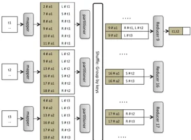
Example 3. Figure 3 gives an example using three
tu-plest1, t2, t3 given the reducer configuration in Figure 1(b). Tuplest1 andt2 have the same blocking key value a1, while
t3 has blocking key value a2. Same as Example 2, t1 has anchor pointa= 2, whilet2, t3 have the same anchor point
a = 4. The key-value pairs generated by the mappers are the same as Figure 2, except the key now is a composite key
Figure 3: PJ-Dedup example using three tuples, given the reducer configuration in Figure 1(b)
that contains the blocking key value. The partitioners will group by the composite key, and determine the destination reducer of a particular key-value pair based only on the re-ducer id component of the composite key. Inside a rere-ducer, there could be multiple reduce tasks, depending on the num-ber of distinct blocking key values received. Reducer 9, for instance, has two reduce tasks. The tuplest1 andt3will not be compared, since they reside in different blocks and thus in different reduce tasks.
Theorem 4. PJ-Dedup achieves with high probabilityX ≤ (1 +o(1)) √ 2n √ k ≤(1 +o(1)) √ 2kXlow, andY ≤(1 +o(1))Wk ≤ (1 +o(1))Ylow.
We give the detailed proof in Appendix B.
Theorem 4 shows thatPJ-Dedup is optimal with respect toY, but can be much worse in terms ofX. For example, if we have many small blocks, then the number of comparisons will beW =O(n), in which case the input size forPJ-Dedup will be larger than the lower bound, by a factor of√2k. On the other hand, if we have few large blocks, andW = Θ(n2),
PJ-Dedup will have an asymptotically optimal input size as well. Our proposed strategy,Dis-Dedup, which we describe next, achieves the best of both worlds.
h1 h2 h3 X Y X Y X Y Lower bounds nk Wk √ 2n √ k W k √ βn k W k Naive-Dedup nk W k n W βn k βW k PJ-Dedup √ 2n √ k W k √ 2n √ k W k √ 2n √ k W k Table 1: Three example blocking functions Example 4. Consider the following three blocking func-tions that generate blocks of different sizes:
(1) The first blocking functionh1 producesβkblocks, for an integerβ >1. The sizes of every block are the same, that is,|Bi|=βkn for alli∈[1, βk]. The lower bound in this case
isXlow ≥max(nk, √ 2W √ k ) = n k andYlow = W k. For N
aive-Dedup, every reducer receives β blocks. Therefore, X = n k
andY = Wk, which is optimal. For PJ-Dedup, regardless of the blocking function,X =
√ 2n √ k andY = W k.
(2) The second blocking function h2 produces only one block of size n. The lower bound in this case is Xlow ≥
max(n k, √ 2W √ k ) = n √ k andYlow= W
k. For Naive-Dedup, one
reducer does all the work, and thusX =nandY =W. (3) The third blocking function h3 produces kβ blocks of equal size for some 1 ≤ β < k, that is, |Bi| = βnk for
all i ∈ [1,k
β]. The lower bound in this case is Xlow =
max(n k, √ 2W √ k ) = √ βn k and Ylow = W k. For Naive-Dedup,
one block is assigned to one reducer, which performs a lo-cal self-join the block it receives, leading to X = βnk and
Y = βWk , both of which are not bounded. For PJ-Dedup
Y is optimal, but X is a factorq2k
β away from the lower
bound.
The comparison is summarized in Table 1. Forh1,N
aive-Dedup matches the lower bounds for bothX andY; forh2,
PJ-Dedup matches the lower bounds; and for h3, neither matches the lower bounds.
Example 4 demonstrates that (1) when the block sizes are small and uniform, such as the ones produced byh1, we should use one reducer to handle each block, as in N aive-Dedup; (2) when there are dominating blocks, such as the ones produced by h2, we should use multiple reducers to divide the workload, as in PJ-Dedup; and (3) when there are multiple relatively large blocks, we should use multiple reducers to handle every large block to avoid unbalanced computation. However, using all kreducers for every large block sends more tuples than necessary, since tuples from different blocks might be sent to same reducer, even though they will not be compared, as inPJ-Dedup.
4.3
The Proposed Strategy
Dis-Dedup adopts a distribution strategy which
guaran-tees that bothX andY are always within a constant factor fromXlow andYlow, by assigning reducers to blocks in
pro-portion to the workload of every block.
Intuitively, since we want to balance computation, a block of a larger size needs more reducers than a block of a smaller size. Since the blocks are independent, we allocate the re-ducers to blocks in proportion to their workload, namely, blockBi will be assigned toki= WWik reducers. However,
ki might not be an integer, and it is meaningless to
allo-cate a fraction of reducers. Thus, ki needs to be rounded
to an integer. Ifki>1, we can assignbkic ≥1 reducers to
Bi. On the other hand, if ki ≤ 1, which meansbkic = 0,
we must still assign at least one reducer to Bi. The total
number of reducers after rounding might be greater thank, in which case reducers have to be responsible for more than one block. Therefore, we need an effective way of assigning reducers to blocks, such that bothX andY are minimized. Ifki≤1, we callBiasingle-reducer block; otherwise,Bi
is amulti-reducer block. LetBsandBlbe the set of
single-reducer blocks and multi-single-reducer blocks respectively. Next, we show how to handle single-reducer blocks and multi-reducer blocks separately, such thatX and Y are bounded by a constant factor. Bs={Bi|Wi≤ W k }, Bl={Bi|Wi> W k }
For the sake of convenience, assume that we have ordered the blocks in increasing order of their workload:W1≤W2≤
be the total amount of workload for multi-reducer blocks, and Ws = Pci=1Bi be the total amount of workload for
single-reducer blocks. Also, letXs (resp. Xl) be the
max-imum number of tuples from single-reducer blocks (resp. multi-reducer blocks) received by any reducer; and let Ys
(resp. Yl) be the maximum number of comparisons from
single-reducer blocks (resp. multi-reducer blocks) performed by any reducer. Therefore,X≤Xs+XlandY ≤Ys+Yl.
4.3.1
Handling multi-reducer blocks
Every blockBi ∈ Bl has ki ≥1 reducers assigned to it,
and we will usekireducers to distributeBivia the triangle
distribution strategy in Section 3. Ifki is fractional, such
aski = 3.1, we will simply usebkic reducers to handleBi.
SincePm
i=c+1ki≤k, every reducer will exclusively handle at most one multi-reducer block.
Example 5. Recall the blocking function h3 in Exam-ple 4: every block is large, sinceWi>Wk. Instead of using
allkreducers to handle every block, we now useki= WWi =β
reducers to handle block√ Bi. Thus, we have X = Xl =
2 √ ki |Bi|= √ 2β k n, andY =Yl= Wi ki = W k. Compared to the
lower bound, we see that Y is optimal, and X is only √2 away from optimal.
In fact, we can be even more aggressive in assigning re-ducers to big blocks, by assigning ki = WWi
l (instead of
ki = WiW) reducers to Bi. This still guarantees that there
is at least one reducer for every multi-reducer block, and one reducer handles at most one multi-reducer block, since Pm
i=c+1ki=k. By handling multi-reducer blocks this way,
Dis-Dedup achieves the following bounds forXlandYl: Theorem 5. Dis-Dedup has with high probability Yl ≤
(1 +o(1))2Ylow andXl≤(1 +o(1))2
√ 2Xlow
Proof. From the analysis of the triangle distribution
strat-egy, we know that with high probabilityYl will be an (1 +
o(1)) factor away from the following quantity:
m max i=c+1 Wi ki = maxm i=c+1 Wi bWi Wlkc ! ≤ maxm i=c+1 2Wi Wi Wlk ! = 2Wl k
As forXl, we know again that with high probability it will
be an (1 +o(1))√2 factor from: m max i=c+1 |Bi| √ ki ≤ √ Wl √ k · m max i=c+1 2|Bi| p |Bi|(|Bi| −1)/2 ! = (1 +o(1))2 √ 2Wl √ k
Note that in the proof, we used bkic ≥ ki/2, which has
accounted for the utilization rate (which is at least 0.5) when bkiccannot be arranged in a triangle. Comparing this with
the lower bounds in Theorem 3, we conclude the proof.
4.3.2
Handling single-reducer blocks
For every blockBi∈ Bs, since we assignki≤1 reducers
to it, we can use one reducer to handle every single-reducer block, just like Naive-Dedup does. However, we must as-sign single-reducer blocks to reducers to ensure that every reducer has about the same amount of workload.
We first present adeterministic distribution strategy for single-reducer blocks, which achieves a constant bound for
XsandYs. However, the deterministic strategy requires the
mappers to keep the ordering of the sizes of single-reducer blocks in memory, which is very costly. We next consider a randomized distribution, which is cheaper to implement, but whose bound for X is dependent on k. Finally, we introduce a hybrid distribution strategy that uses the ran-domized distribution for most of the single-reducer blocks, and the deterministic distribution for only a small subset of the single-reducer blocks. The hybrid distribution requires a small memory footprint, and in the same time achieves constant bounds for bothXs andYs.
Deterministic Distribution. In order to allocate the
single-reducer blocks evenly, we first order thecsingle-reducer blocks according to their block sizes, and divide them into
g= c k groups
3
, where each group consists of consecutivek
blocks in the ordering. Then, we assign to each reducer g
blocks, one from each group.
Theorem 6. The deterministic distribution strategy for single-reducer blocks achievesYs≤2Ylow andXs≤2Xlow.
Proof. Recall that we started by ordering the blocks in
increasing size. Hence, we have that Xs≤Pgi=1|Bi·k|and
Ys≤Pgi=1Wi·k.
LetWs=Pci=1Wi, and observe thatkPig=1−1Wi·k≤Ws.
Also, Wg·k ≤ W/k. Thus, Ys ≤ 2Wk. Similarly, for the
input sizes we have thatPg
i=1|Bi·k| ≤ Pc i=1|Bi|/k+Bc≤ n k + √ 2W √ k ≤2 max( n k, √ 2W √ k ).
The problem with implementing the deterministic distri-bution is that there can be a large number of single-reducer blocks, and keeping track of the ordering of all block sizes is an expensive task within each mapper, not to mention the need to actually order all the single-reducer blocks.
Randomized Distribution. This algorithm simply
dis-tributes each single-reducer block to a reducer by using a random hash function. In order to analyze the randomized distribution, it suffices to consider the worst-case scenario, which is when we have k single-reducer blocks, each with |Bi|=n/k. In this case, the problem becomes a
balls-into-bins scenario, where we have k balls (blocks) that we dis-tribute independently and uniformly at random intokbins (reducers). It then holds [26] that with high probability each reducer will receiveO(ln(k)) blocks. Thus:
Theorem 7. The randomized distribution strategy for single-reducer blocks achievesYs≤ln(k)YlowandXs≤ln(k)Xlow.
The randomized method is efficient in practice, since we do not have to keep track of the single-reducer blocks, but we are adding (in the worst case) an additional ln(k) factor.
Hybrid Distribution. The hybrid algorithm combines
the randomized and deterministic distribution to achieve ef-ficiency and almost optimal distribution. To start, we set a threshold τ = W
3kln(k).
4 For the blocks whereW
i≥τ (but
3We assume that c
k is an integer; otherwise, we can
con-ceptually add less thankempty blocks toBs to make ck an
integer, and the analysis remains intact.
4The threshold value is chosen as a result of the connection to the weighted balls-into-bins problem. When we throw
k balls of weight W/k into k bins uniformly at random, the expected maximum number of balls isO(ln(k)), and so the maximum weight isO(Wln(k)/k). If we instead throw
kln(k) balls of weight W/kln(k), the expected maximum number remainsO(ln(k)), but since the balls are of smaller weight the maximum weight decreases toO(W/k).
Algorithm 2Dis-Dedup
1: classMapper
2: BKV2RIDs←empty dictionary
3: methodMapperSetup(HM1,HM2)
4: Wl←P
bkv∈HM1.keySet()HM1[bkv]
5: S← {1,2, . . . , k}
6: for allbkv∈HM1.keySet()do
7: ki← bHM1[bkv] Wl kc
8: RIDSi←selectkielements fromS
9: BKV2RIDs[bkv]←RIDSi
10: S←S−RIDSi
11: SortedBKV s←sort all keys inHM2
12: RID←0
13: for allbkv∈SortedBKV sdo
14: BKV2RIDs[bkv]←RID%k
15: RID←RID+ 1
16: methodMap(Tuplet,null)
17: bkv←h(t)
18: ifBKV2RIDs[bkv]6=∅then
19: rid←a random number from [1, k]
20: Emit(Keyrid#bkv, S#Tuplet)
21: else
22: RIDs←BKV2RIDs[bkv]
23: ki←RIDs.size()
24: li←the large integer s.t.li(li−1)/2< ki
25: Inta←a random value from [1, li]
26: for allp∈[1, a)do
27: ridIndex←rid of Reducer [p, a]
28: rid←RIDs[ridIndex]
29: Emit(Keyrid#bkv, L#Tuplet)
30: ridIndex←rid of Reducer [a, a]
31: rid←RIDs[ridIndex]
32: Emit(Keyrid#bkv, S#Tuplet)
33: for allq∈(a, l]do
34: ridIndex←rid of Reducer [a, q]
35: rid←RIDs[ridIndex]
36: Emit(Keyrid#bkv, R#Tuplet)
37: classPartitioner
38: methodPartition(Keyrid#bkv,Valuev, k)
39: Returnrid
40: classReducer
41: methodReduce(Keyrid#bkv,Values [v1, v2. . .]) 42: same as the reduce function in Algorithm 1
stillWi≤ Wk), we use the deterministic distribution, while
for the blocks whereWi< τ we use the randomized
distri-bution. Observe that now the deterministic option is much cheaper, since we have to keep track of at most 3kln(k) blocks (which number depends only on the number of re-ducers, and notn).
Theorem 8. The hybrid distribution strategy for single-reducer blocks has with high probabilityYs≤(1 +o(1))2Ylow
andXs≤(1 +o(1))3Xlow.
Proof. Applying a result from [4] on the weighted balls-into-bins problem, we obtain that with high probability for the randomly distributed blocksYsr ≤(1+o(1))Ylow. A
sim-ilar argument for the input size gives usXsr≤(1+o(1))Xlow.
For the deterministically distributed blocks, sinceτ ≤W k,
we can apply Theorem 6 to obtain that Yd
s ≤ 2Ylow and
Xsd≤2Xlow.
4.3.3
Implementation
Dis-Dedup combines the triangle distribution strategy for
multi-reducer blocks and the hybrid distribution for single-reducer blocks. However, given a new tuple ingested by a
mapper, how does the mapper know whether the tuple be-longs to a multi-reducer block or a single-reducer block? In order to make this decision, we need some preprocessing to collect statistics to be loaded into each mapper. In partic-ular, we need to compute the blocking key values of every multi-reducer block Bi ∈ Bl, and the associated workload
Wi. Let HM1 denote the HashMap data structure that stores the mapping from a blocking key value in the multi-reducer blocks to the size of the block. In addition, we need the blocking key values of those single-reducer blocks
Bi∈ Blthat haveWi≥τ, and the associated workloadWi,
in order to implement the hybrid distribution strategy for the single-reducer blocks. Let HM2 denote the HashMap data structure that stores the mapping from a blocking key value to the size of the block.
To computeHM1 and HM2, we use three simple word-count alike MapReduce jobs. The first job takes the original dataset as input, and counts the size of every blockBi. The
second job takes as input the result of the first job, and counts the total workloadW. The third job takes as input the result of the first job andW, and outputs the blocks for which Wi > Wk, namely HM1, and also the blocks where
W
3kln(k) < Wi≤
W
k, namelyHM2.
Algorithm 2 describes in detail theDis-Dedup distribution strategy. The mapper now has a setup method that needs to be executed, which allocates reducers to blocks inHM1 and
HM2 (Lines 3-15). To allocate reducers to blocks inHM1, we first compute the sum of workload of all the multi-reducer blocks, i.e., Wl (Line 4). For every blocking key value in
HM1, we calculate the number of reducers ki allocated to
it, and selectkireducers from the set ofkreducers (Lines
5-10). For every blocking key value inHM2, we first sort them based on their workload (Line 11), and allocate one reducer to the sorted blocks in a round-robin manner (Lines 12-15). In the actual mapping function, given a new tupletand its blocking key value bkv, we check if we have a fixed set of reducers allocated to it. If there is no such fixed allocation,
bkv must the block that is randomly distributed, and thus we randomly choose a reducer to send the tuple (Lines 18-20). If there is a fixed set of reducerRIDsallocated to it, we distributetaccording toPJ-Dedup, by arranging reducer
RIDs in a triangle (Lines 22-36). The partitioner sends a key-value pair according to theridpart in the key (Lines 37-39). The reducer is the same as that of Algorithm 1 (Lines 40-42).
Theorem 9. Dis-Dedup with hybrid distribution for single-reducer blocks achieves with high probability X ≤ cxXlow,
andY ≤cyYlow, wherecx= 3+2
√
2+o(1)andcy= 4+o(1).
Theorem 9 is obtained by combining Theorems 5 and 8.
5.
DEDUPLICATION USING
MULTIPLE BLOCKING FUNCTIONS
Since a single blocking function might result in false nega-tives by failing to assign duplicate tuples to the same block, multiple blocking functions are often used to decrease the likelihood of a false negative. In this section, we study how to distribute the blocks produced by s different blocking functionsh1, h2, . . . , hs.A straightforward strategy to handlesblocking functions would be to applyDis-Dedupstimes (possibly simultane-ously). However, this straightforward strategy has two prob-lems: (1) it fails to leverage the independence of the blocking
functions, and the tuples from blocks generated by different blocking functions might be sent to same reducer, where they will not be compared. This is similar to PJ-Dedup’s failure to leverage the independence of the set of blocks gen-erated by a single blocking function, as shown in Example 4; and (2) a tuple pair might be compared multiple times, if that tuple pair belongs to multiple blocks, each from a dif-ferent blocking function. We address these two problems by two principles: (1) allocating reducers to blocking func-tions proportional to their workload; and (2) imposing an ordering of the blocking functions.
Reducer Allocation. We allocate one or more reducers
to a blocking function in proportion to the workload of that blocking function, similar to Dis-Dedup discussed in Sec-tion 4. Let mj denote the number of blocks generated by
a blocking functionhj,Bji denote the i-th block generated
byhj, and Wij =
|Bij| 2
denote the workload of Bij. Let
Wj=Pmj i=1W
j
i be the total amount of workload generated
byhj, andW =Ptj=1Wj be the total workload generated
by alltblocking functions. Therefore, the number of reduc-ersBijgets assigned is W
j i Wj · Wj W k, where Wj W kis the number
of reducers for handling the blocking function hj. Thus,
the number of reducers assigned toBji is W
j i
W , regardless of
which blocking function it originates from.
This means that we can view the blocks from multiple blocking functions as a set of (possibly overlapping) blocks produced by one blocking function, and apply Dis-Dedup as-is. The only modification needed is that in the mapper of
Dis-Dedup, instead of applying one hash function to obtain one blocking key value, we applyshash functions to obtain
sblocking key values (we also need to apply the body of the mapping function for every blocking key value). We call the slightly modified version of Dis-Dedup to handle multiple blocking functionsDis-Dedup+.
Theorem 10. Fortblocking functions,Dis-Dedup+achieves
X <((3 + 2√2)s+o(1))Xlow, andY = (4 +o(1))Ylow. Proof. The lower bound forXandY forsblocking func-tions is the same lower bound for single blocking function, as stated in Theorem 9, exceptW now denotes the total num-ber of comparisons for allsblocking functions. The proof of Theorem 10 follows the same line as the proof of Theorem 9. The only difference is when we are dealing withBs: instead
of having the inequalityPc
i=1|Bi|< nfor a single blocking
function, we now have Pc
i=1|Bi| < sn, which leads to an additional factorsin the bound forX.
The above analysis tells us that the number of compar-isons will be optimal, but the input may have to be repli-cated as many as s times. The reason for this increase is that the blocks may overlap, in which case tuples that be-long in multiple blocks may be replicated. The results from Theorem 10 can be carried to a single blocking function that produces a set of overlapping blocks, wheres=
Pm
i=1|Bi|
n .
Blocking Function Ordering. Since a tuple pair can
have the same blocking key values according to multiple blocking functions, a tuple pair can occur in multiple blocks. To avoid producing the same tuple pair more than once, we impose an ordering of the blocking functions, from h1 to
hs. A tuple pair only gets compared according to thelowest
numbered blocking function that assigns that tuple pair in the same block.
Example 6. Suppose two tuplest1andt2are in the same block according to the blocking functions h2, h3, h5, namely,
h2(t1) = h2(t2), h3(t1) = h3(t2) and h5(t1) = h5(t2). In this case, we only comparet1 andt2 in the block generated by h2, and omit the comparison of those two tuples in the blocks generated byh3 andh5.
In order to recognize which blocking function generated a tuple pair comparison inside a reduce task, we augment the key of the mapper fromrid#hkvtorid#hkv#hIndex, where hIndexis the blocking function number that gener-ated this hkv. In the reduce function, before a tuple pair is compared, we check if there is another blocking function whose index is smaller than thehIndexthat puts that tuple pair in the same block. If such a blocking function exists, we skip the comparison.
6.
EXPERIMENTAL STUDY
In this section, we evaluate the effectiveness of our dis-tribution strategies. All experiments are performed on a cluster of eight machines, running Hadoop 2.6.0 [1]. Each machine has 12 Intel Xeon CPUs at 1.6 GHz, 16MB cache size, 64GB memory, and 4TB hard disk. All machines are connected to the same gigabit switch. One machine is ded-icated to serve as the resource manager for YARN and as the HDFS namenode, while the other seven are slave nodes. The HDFS block size is the default 64MB, and all machines serve as data nodes for the DFS. Every node is configured to be able to run 7 reduce tasks at the same time, and thus in total, 49 reduce tasks can run in parallel. Our cluster re-sembles the cluster that is used in production by Thomson Reuters to perform data deduplication. We also use a real dataset from that company, as described next.
Datasets. We design asynthetic datagenerator, which
takes as input the number of tuplesn, the number of blocks
m, and a parameterθ controlling the distribution of block sizes, following the zipfian distribution. Every generated tuple has two columns {A, B}. Column A is the blocking key attribute, whose values range from 1 tom. The blocking functionhfor a tupletin the synthetic dataset ish(t) =t[A]. Thus, tuples with the same value forAbelong to the same block. Column B is a randomly generated string of 1000 characters. The comparison between two tuples is the edit distance between the two values forB.
We use two real datasets. The first one is a list of publica-tion records from CITESEERX 5, calledCSX. The second one, calledOA, is a private dataset from Thomson Reuters, containing a list of organization names and their associ-ated information, such as addresses and phone numbers, ex-tracted from news articles. CSXuses the publication title as the blocking key attribute, whileOAuses the organization name. The blocking function for both datasets uses min-Hash [18]. A minmin-Hash signature is generated for each tuple, and tuples with the same signature belong in the same block. For each tuple inCSXorOA, the blocking function extracts 3-grams from the blocking key attribute, and applies a ran-dom hash function to the set of 3-grams; the minimum hash value for the set of 3-grams is used as the minHash signature for that tuple. We can generate multiple blocking functions by using different random hash functions. The comparison between two tuples is the edit distance between the two val-ues of the blocking key attributes.
5
0 5 10 15 20 25 30 35 40 45 50 10 15 20 25 30 35 40 45 50 X (in thousands)
numTuples (in thousands)
Naive-Dedup PJ-Dedup Dedoop (a) Exp-1: X 0 200 400 600 800 1000 1200 1400 1600 1800 2000 10 15 20 25 30 35 40 45 50 Y (in millions)
numTuples (in thousands)
Naive-Dedup PJ-Dedup Dedoop (b) Exp-1: Y 0 500 1000 1500 2000 2500 3000 3500 4000 4500 10 15 20 25 30 35 40 45 50
Time (in seconds)
numTuples (in thousands)
Naive-Dedup PJ-Dedup Dedoop (c) Exp-1: time 5 10 15 20 25 30 35 40 45 50 20 30 40 50 60 70 80 X (in thousands) numReducers PJ-Dedup Dedoop (d) Exp-2: X 150 200 250 300 350 400 450 500 550 20 30 40 50 60 70 80 Y (in millions) numReducers PJ-Dedup Dedoop (e) Exp-2: Y 400 600 800 1000 1200 1400 1600 1800 20 30 40 50 60 70 80
Time (in seconds)
numReducers PJ-Dedup Dedoop (f) Exp-2: time 0 50 100 150 200 250 100 1000 10000 100000 1e+06 1e+07
Time (in seconds)
numBlocks (in log scale) Naive-Dedup PJ-Dedup Dis-Dedup Dedoop (g) Exp-3 0 500 1000 1500 2000 2500 3000 3500 4000 4500 0.25 0.3 0.35 0.4 0.45 0.5 0.55 0.6 0.65 0.7 X (in thousands) Theta Naive-Dedup PJ-Dedup Dis-Dedup (h) Exp-4: X 0 200 400 600 800 1000 1200 0.25 0.3 0.35 0.4 0.45 0.5 0.55 0.6 0.65 0.7 Y (in millions) Theta Naive-Dedup PJ-Dedup Dis-Dedup (i) Exp-4: Y 0 200 400 600 800 1000 1200 1400 1600 1800 0.25 0.3 0.35 0.4 0.45 0.5 0.55 0.6 0.65 0.7
Time (in seconds)
Theta Naive-Dedup PJ-Dedup Dis-Dedup (j) Exp-4: time 100 150 200 250 300 350 400 450 500 20 30 40 50 60 70 80
Time (in seconds)
numReducers Naive-Dedup PJ-Dedup Dis-Dedup (k) Exp-5: Synthetic 0 100 200 300 400 500 600 700 20 30 40 50 60 70 80
Time (in seconds)
numReducers Naive-Dedup PJ-Dedup Dis-Dedup (l) Exp-5: CSX 100 200 300 400 500 600 700 20 30 40 50 60 70 80
Time (in seconds)
numReducers Naive-Dedup PJ-Dedup Dis-Dedup (m) Exp-5: OA 0 1000 2000 3000 4000 5000 6000 7000 0 2 4 6 8 10 12 14 16 18 20 X (in thousands) Naive-Dedup+ PJ-Dedup+ Dis-Dedup+ (n) Exp-6: X 0 1000 2000 3000 4000 5000 6000 7000 0 2 4 6 8 10 12 14 16 18 20 Y (in millions) Naive-Dedup+ PJ-Dedup+ Dis-Dedup+ (o) Exp-6: Y 0 500 1000 1500 2000 2500 3000 0 2 4 6 8 10 12 14 16 18 20
Time (in seconds)
Naive-Dedup+ PJ-Dedup+ Dis-Dedup+
(p) Exp-6: time
Figure 4: Evaluating Distribution Strategies
Table 2 summarizes the statistics for each dataset we used for performing data deduplication using a single blocking function in Section 6.2. We will use up to 20 blocking functions for performing data deduplication using multiple blocking functions in Section 6.3.
Dataset # Tuples AVG block size MAX block size
CSX 1.4M 1.75 35021
OA 7.4M 1.31 7969
Synthetic 20M 4 3967
Table 2: Datasets Statistics
Algorithms. We compare the following distribution
strate-gies: (1) Naive-Dedup is the na¨ıve distribution strategy, where every block is assigned to one reducer; (2)PJ-Dedup is the proposed strategy where every block is distributed us-ing the triangle distribution strategy, which is strictly better
than applying existing parallel join algorithms [2, 25]; (3)
Dis-Dedup is the proposed distribution strategy for a single blocking function, which is theoretically optimal; (4)
De-doop [20] is the state-of-the-art MapReduce algorithm for performing blocking using MapReduce. Dedooponly opti-mizes forY by dividing all the tuple pairs needed to be com-pared intokequal parts, and assigning each part to one re-ducer. The details ofDedoopcan be found in Appendix C; and (5) Dis-Dedup+,
Naive-Dedup+, and PJ-Dedup+ are
extensions of Dis-Dedup, Naive-Dedup, andPJ-Dedup, re-spectively for multiple blocking functions. Dis-Dedup+ is described in Section 5. Naive-Dedup+ and
PJ-Dedup+
em-ploy the blocking function ordering technique described in Section 5 to avoid comparing a tuple pair multiple times.
Since the distribution strategies are random, we run each experiment three times, and report the average. The time to
compute the necessary statistics forDis-Dedup andDedoop is included in the running time ofDis-Dedup andDedoop, respectively.
6.1
Single Block Deduplication Evaluation
In this section, we compareNaive-Dedup,PJ-Dedup, andDedoopwhen performing a self-join on the synthetic dataset.
We omitDis-Dedup, since it is identical toPJ-Dedup when there is only one block.
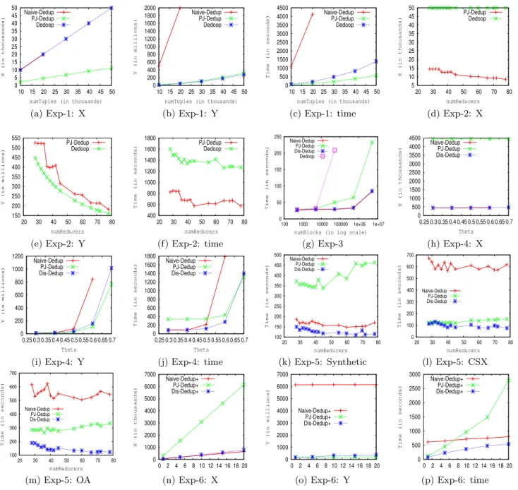
Exp-1: Varying number of tuples. Figure 4(a-c)
shows the parametersX,Y, andtimeforNaive-Dedup,P J-Dedup, andDedoopfork= 45 reducers. We terminate a job after 6000 seconds. As we can see in Figure 4(c),N aive-Dedup exceeds this time limit after 30K tuples, since the computation occurs only in a single reducer. In terms of the maximum input size X, Figure 4(a) shows thatPJ-Dedup achieves the best behavior, while forNaive-Dedup and
De-doopX is equal to the number of tuplesn. Indeed,N aive-Dedup uses one reducer to do all the work, andDedoophas one reducer that gets assigned the first n(n2−k1) tuple pairs, which need to access allntuples. In terms ofY, as depicted in Figure 4(b),Naive-Dedup performs the worst. Dedoopis slightly better thanPJ-Dedup, since it distributes the com-parisons evenly amongst all reducers, whilePJ-Dedup has more work for reducers indexed (p, q) than reducers indexed (p, p).
The running time of all three algorithms is depicted in Fig-ure 4(c), and it shows thatPJ-Dedup achieves the best per-formance. In fact, comparing Figure 4(a) with Figure 4(c), we can see that as the number of tuples increases, the gap betweenPJ-Dedup andDedoopin terms of the input size
Xgrows, and so does the running time. This indicates that whenY is similar forPJ-Dedup andDedoop, the input size
X becomes the differentiating factor.
Exp-2: Varying number of reducers. Figure 4(d-f)
shows the effect of the number of reducers on the parame-tersX,Y, andtime for bothPJ-Dedup andDedoop. We fix the number of tuples to be n = 50K. The first ob-servation is that PJ-Dedup outperforms Dedoop for any
k, as shown in Figure 4(f). In fact, PJ-Dedup runs 2X faster thanDedoop. Second, both X and Y are decreas-ing forPJ-Dedup as k increases. However, the decrease is not smooth across the values ofkand we can observe a few dips fork= 36,45,55,66,78. This behavior occurs because
PJ-Dedup arranges thek reducers in a triangle. Since for
certain values ofk this is not possible, we choose then the largest subset of reducers that can be arranged into a trian-gle, and thus waste a small fraction of reducers.
Finally, as we can see from Figure 4(f), the running time improves ask increases fork <50, and fluctuates ask in-creases whenk >50. This is because our cluster has a max-imum number of 49 reducers being able to run in parallel. Ifk >50, not all reducers can start at once; some reducers can only start after reducers in the first round finish.
Memory. An important requirement for any MapReduce
job is to have sufficient memory for each reducer. The maxi-mum memory requirements for all algorithms are linear with respect to X, sinceX represents the maximum number of tuples that need to be stored in the heap space of a reducer. As we can see from Figure 4(a), PJ-Dedup requires much less memory than Dedoop. Indeed, for Dedoopat least one reducer needs to store allntuples, while the heap space required for PJ-Dedup is O(√n
k), which not only is much
smaller than O(n), but also decreases as k increases (this can be seen in Figure 4(d)).
6.2
Evaluating Deduplication
using Single Blocking Function
In this section, we compareNaive-Dedup,PJ-Dedup,D is-Dedup, andDedoopfor deduplication using a single block-ing function on all three datasets.
Exp-3: Varying number of blocks. In this
experi-ment, we fix the number of tuples per block to be 4, and then vary the number of blocks, using the synthetic dataset. As shown in Figure 4(g),Dedoopfails (heap space error) af-ter 500,000 blocks. This is becauseDedoopkeeps the sizes of every block in the memory of every mapper and reducer in order to evenly distribute the tuple pairs; this footprint grows as the number of blocks increases. We therefore omit
Dedoopfrom the rest of the experiments in this section. Dis-Dedup is identical toNaive-Dedup in this experiment, since all block sizes are the same, and hence no multi-reducer blocks exist. Dis-Dedup is better thanPJ-Dedup, since the input sizeXforDis-Dedup, which isn
k, is smaller than that
forPJ-Dedup, which is √
2n
√
k.
Exp-4: Varying block size distribution. In order
to test how different algorithms handle block-size skew, we vary the distribution of the block sizes by varying the pa-rameter θ for the synthetic dataset, using n = 20M tu-ples, and 5M blocks. Figure 4(h) shows that Dis-Dedup andNaive-Dedup send less tuples thanPJ-Dedup, and Fig-ure 4(i) shows that the number of comparisonsY increases as the data becomes more skewed across all three algorithms. However,Y forPJ-Dedup grows at the lowest rate, andY
forDis-Dedup is just a little worse thanPJ-Dedup. In terms of running, time, Figure 4(j) shows that when the data is not skewed (θ= 0.3,0.4),Naive-Dedup andDis-Dedup perform the best, since X is now the differentiating factor. When the data becomes more skewed (θ= 0.5),Dis-Dedup starts performing better than Naive-Dedup, which is still better thanPJ-Dedup. Asθfurther increases (θ= 0.6,0.7),Y be-comes the dominating factor in terms of running time. Thus, the running time forNaive-Dedup degrades fast, whileD is-Dedup andPJ-Dedup have similar performance. This ob-servation supports our theoretical analysis thatDis-Dedup can adapt to all levels of skew, whileNaive-Dedup andP J-Dedup perform well only at one end of the spectrum.
Exp-5: Varying number of reducers. In this
experi-ment, we vary the number of reducersk, and compareN aive-Dedup,PJ-Dedup, andDis-Dedup using all three datasets. For the synthetic dataset, we usedn= 20M,m= 5M, and
θ= 0.5. Figure 4(k-m) shows thatDis-Dedup is consistently the best algorithm for all three datasets, and any number of reducers. For the synthetic dataset,Naive-Dedup performs better thanPJ-Dedup, while for the two real datasets the opposite behavior occurs, since the number of multi-reducer blocks inCSXandOAis bigger than that of the synthetic dataset. Another interesting trend to note here is that as the number of reducerskincreases, the difference in running time between Dis-Dedup and PJ-Dedup also grows. The reason for this behavior is that X forPJ-Dedup is a √2k
factor away from the bound Xlow, and thus dependent on
k, whileX forDis-Dedup is only a constant factor 2 away.
6.3
Evaluating Deduplication
In this section, we compare the algorithmsNaive-Dedup+,
PJ-Dedup+, andDis-Dedup+ in the case of multiple block-ing functions, usblock-ing the two real datasets.
Exp-6: Varying the number of blocking functions.
Figure 4(n-p) shows the comparison usingCSX. The input sizeX of all three algorithms increases linearly w.r.t. the number of blocking functions, as shown in Figure 4(n), while theY of all three algorithms increases very little, as shown in Figure 4(o). This behavior is observed because many tuple pairs generated by a blocking function have already been compared in previous blocking functions, and are thus skipped. Table 3 shows the total number of comparisonsW
for various numbers of blocking functions, indicating that the new tuple pair comparisons generated by 20 blocking functions is not much larger than the comparisons generated by 1 blocking function.
Figure 4(p) shows the running time comparison. D is-Dedup+achieves the best performance across any number of blocking functions. As the the number of blocking functions increases, the gap betweenNaive-Dedup+ and
Dis-Dedup+
becomes smaller, while the gap between PJ-Dedup+ and
Dis-Dedup+ becomes larger. The reason is that the multi-reducer blocks ford1blocking functions may become single-reducer blocks ford2> d1blocking functions asW becomes larger. Therefore, distributing those blocks to one reducer, asNaive-Dedup+does, instead of distributing them to mul-tiple reducers, asPJ-Dedup+ does, becomes more efficient. Varying number of blocking functions using theOAdataset shows similar results, and is reported in Appendix D.
Dataset 1 5 10 15 20
CSX 667.45 710.64 741.52 768.51 784.40
OA 66.16 67.24 67.92 68.00 68.06
Table 3: Total number of comparisons W (in
mil-lions), for different number of blocking functions
7.
RELATED WORK
Data deduplication has been extensively covered in many surveys [23, 11, 10, 24, 12, 16, 17]. To avoid n2 compar-isons, blocking methods partition all records into disjoint blocks; only records within the same block are compared, while records residing in different blocks are considered non-duplicates [3, 5]. While blocking techniques speed up com-putation by avoiding the comparison between certain tuple pairs, performing deduplication using a parallel framework can obtain even further speed ups. In this context,
De-doop [20, 21] targets deduplication on MapReduce. De-doopevenly distributes the comparisonsY at the cost of an increased input sizeX. In addition, in order to decide which tuple pairs are compared by each reducer, every mapper and reducer ofDedoophas to keep detailed block size distribu-tion statistics in memory, which could be as large asO(n), renderingDedoopinfeasible to run for large datasets.
Parallel join processing, such as similarity joins [27, 31], theta-joins [25], and multi-way natural joins [2], is another line of relevant work, since one can view the distributed blocking problem as a self-join, where the joining attribute is the blocking key attribute. However, most of the work on parallel join processing [25, 2] is for two-table joins, so the techniques are not directly applicable to self-join with-out wasting almost half of the available workers, as shown in Section 3. Our proposed triangle distribution strategy is a non-trivial adaptation of the existingShares distribution strategy [2] for theR×Sjoin with theoretical guarantees on
both the communication costX and the computation cost
Y. In addition, applying even the adapted self-join strat-egy on blocks directly without considering the block sizes yields a strategy without constant bound guarantee on X, as shown in Section 4.2. Our proposed Dis-Dedup, how-ever, assigns workers in proportion to the workload of every block to achieve a constant-boundX and Y. Furthermore, dealing with multiple blocking functions basically means to process a disjunction of conjunctive queries, a problem, to the best of our knowledge, is never considered in parallel join processing.
8.
CONCLUSION AND FUTURE WORK
In this paper, we study the problem of performing block-ing for data deduplication usblock-ing a shared-nothblock-ing distributed computing framework. We develop a cost model that cap-tures both the communication cost and computation cost. Under this cost model, we propose theDis-Dedup algorithm, which guarantees that the input sizeX and the number of comparisonsY per reducer are within a small constant fac-tor from the optimal. Through extensive experiments, we show thatDis-Dedup adapts to data skew, and significantly outperforms any alternative strategy we consider, including the state-of-the-art algorithm.
When there are multiple blocking functions, a large per-centage of compared tuple pairs belong to the same block ac-cording to more than one blocking functions. While our pro-posed strategy avoids producing the same tuple pair more than once, a tuple still needs to be sent as many times as the number of blocking functions. Future work includes gath-ering statistics about the overlapping of blocks, so that we can merge largely overlapping blocks to further reduce the communication cost.
9.
REFERENCES
[1] Apache hadoop.http://hadoop.apache.org. [2] F. N. Afrati and J. D. Ullman. Optimizing joins in a
map-reduce environment. InEDBT, pages 99–110, 2010. [3] R. Ananthakrishna, S. Chaudhuri, and V. Ganti.
Eliminating fuzzy duplicates in data warehouses. InVLDB, pages 586–597, 2002.
[4] P. Beame, P. Koutris, and D. Suciu. Skew in parallel query processing. In R. Hull and M. Grohe, editors,PODS, pages 212–223. ACM, 2014.
[5] M. Bilenko, B. Kamath, and R. J. Mooney. Adaptive blocking: Learning to scale up record linkage. InICDM, pages 87–96, 2006.
[6] P. Christen. A survey of indexing techniques for scalable record linkage and deduplication.IEEE Trans. on Knowl. and Data Eng., 24(9):1537–1555, Sept. 2012.
[7] S. Chu, M. Balazinska, and D. Suciu. From theory to practice: Efficient join query evaluation in a parallel database system. InSIGMOD, pages 63–78, 2015. [8] J. Dean and S. Ghemawat. Mapreduce: simplified data
processing on large clusters.Communications of the ACM, 51(1):107–113, 2008.
[9] D. J. DeWitt, J. F. Naughton, D. A. Schneider, and S. Seshadri. Practical skew handling in parallel joins. In
VLDB, pages 27–40, 1992.
[10] X. L. Dong and F. Naumann. Data fusion: resolving data conflicts for integration.PVLDB, 2(2):1654–1655, 2009. [11] A. K. Elmagarmid, P. G. Ipeirotis, and V. S. Verykios.
Duplicate record detection: A survey.IEEE Transactions on Knowledge and Data Engineering, 19(1):1–16, 2007. [12] L. Getoor and A. Machanavajjhala. Entity resolution:
theory, practice & open challenges.PVLDB, 5(12):2018–2019, 2012.
[13] D. M. Gordon, G. Kuperberg, and O. Patashnik. New constructions for covering designs.J. COMBIN. DESIGNS, 3(269–284), 1995.
[14] M. A. Hern´andez and S. J. Stolfo. The merge/purge problem for large databases.ACM SIGMOD Record, 24(2):127–138, 1995.
[15] M. A. Hern´andez and S. J. Stolfo. Real-world data is dirty: Data cleansing and the merge/purge problem.Data Mining and Knowledge Discovery, 2(1):9–37, 1998.
[16] T. N. Herzog, F. J. Scheuren, and W. E. Winkler.Data Quality and Record Linkage Techniques. Springer Science & Business Media, 2007.
[17] I. F. Ilyas and X. Chu. Trends in cleaning relational data: Consistency and deduplication.Foundations and Trends in Databases, 5(4):281–393, 2015.
[18] P. Indyk. A small approximately min-wise independent family of hash functions.Journal of Algorithms, 38(1):84–90, 2001.
[19] S. Janson. Large deviations for sums of partly dependent random variables.Random Struct. Algorithms,
24(3):234–248, 2004.
[20] L. Kolb, A. Thor, and E. Rahm. Dedoop: efficient deduplication with hadoop.PVLDB, 5(12):1878–1881, 2012.
[21] L. Kolb, A. Thor, and E. Rahm. Load balancing for mapreduce-based entity resolution. InICDE, pages 618–629, 2012.
[22] H. K¨opcke, A. Thor, and E. Rahm. Evaluation of entity resolution approaches on real-world match problems.
PVLDB, 3(1):484–493, 2010.
[23] N. Koudas, S. Sarawagi, and D. Srivastava. Record linkage: similarity measures and algorithms. InSIGMOD, pages 802–803, 2006.
[24] F. Naumann and M. Herschel.An Introduction to Duplicate Detection. Synthesis Lectures on Data Management. 2010. [25] A. Okcan and M. Riedewald. Processing theta-joins using
mapreduce. InSIGMOD, pages 949–960. ACM, 2011. [26] M. Raab and A. Steger. ”balls into bins” - A simple and
tight analysis. InRANDOM, pages 159–170, 1998. [27] A. D. Sarma, Y. He, and S. Chaudhuri. Clusterjoin: A
similarity joins framework using map-reduce.PVLDB, 7(12):1059–1070, 2014.
[28] A. D. Sarma, A. Jain, A. Machanavajjhala, and P. Bohannon. An automatic blocking mechanism for large-scale de-duplication tasks. InCIKM, pages 1055–1064, 2012.
[29] J. Sch¨onheim. On coverings.Pacific Journal of Mathematics, 14:1405–1411, 1964.
[30] J. D. Ullman. Designing good mapreduce algorithms.
XRDS, 19(1):30–34, Sept. 2012.
[31] R. Vernica, M. J. Carey, and C. Li. Efficient parallel set-similarity joins using mapreduce. InSIGMOD, pages 495–506. ACM, 2010.
[32] S. E. Whang, D. Menestrina, G. Koutrika, M. Theobald, and H. Garcia-Molina. Entity resolution with iterative blocki