85th Annual Conference will be held in Warwick, from 18th – 20th
April 2011.
Impact of Off-farm Income on Farm Efficiency in Slovenia
Štefan Bojneca and Imre Fertőbc
a University of Primorska, Faculty of Management, Cankarjeva 5, 6104 Koper, Slovenia,
email: stefan.bojnec@fm-kp.si, stefan.bojnec@siol.net
b Corvinus University of Budapest, email: imre.ferto@uni-corvinus.hu
cInstitute of Economics, Hungarian Academy of Sciences, Budaörsi u. 45, H-1112 Budapest,
Hungary, email: ferto@econ.core.hu
Copyright 2011 by Štefan Bojnec and Imre Fertő. All rights reserved. Readers may make verbatim copies of this document for non-commercial purposes by any means, provided that this copyright notice appears on all
Impact of Off-farm Income on Farm Efficiency in Slovenia
Štefan Bojneca and Imre Fertőbc
a University of Primorska, Faculty of Management, Cankarjeva 5, 6104 Koper, Slovenia,
email: stefan.bojnec@fm-kp.si, stefan.bojnec@siol.net
b Corvinus University of Budapest, email: imre.ferto@uni-corvinus.hu
cInstitute of Economics, Hungarian Academy of Sciences, Budaörsi u. 45, H-1112 Budapest,
Hungary, email: ferto@econ.core.hu
Abstract:
The paper investigates the impact of off-farm income on farm technical efficiency for the Slovenian Farm Accountancy Data Network farms in the years 2004-2008. Farm stochastic frontier time-varying decay inefficiency is positively associated with total utilised agricultural areas and total labour input, and vice versa with intermediate consumption and fixed assets. We find a positive association between farm technical efficiency and the off-farm income. Farm technical efficiency has increased steadily over time, the process, which was led by the off-farm spill over effect and most efficient farms. Farm technical efficiency is also positively associated with economic farm size, while association with subsidies is mixed depending on the estimation procedure. Quantile regression confirms the positive and significant associations between farm technical efficiency and off-farm income, and between farm technical efficiency and farm economic size, as well as also the positive association between farm technical efficiency and subsidies, but the results are sensitive by quantiles.
Key words:
Off-farm income, Stochastic frontier analysis, Panel regression, Quantile regression, Slovenia
Introduction
Recent literature on rural development explains multifunctional and synergistic function of agricultural households in combination with other sources of employment. The role of non-farm income has increased in the total income of non-farm households in several of developed countries. Income diversification of rural households can be driven by different determinants such as higher returns to labour and/or capital in off-farm economy as well as by risks pertaining to farm input market imperfections. Literature provides evidence on a positive association between off-farm income and farm performance (e.g. Rizov et al., 2001; Rizov and Swinnen, 2004; Hertz, 2009).
Therefore, the motivation for this paper is to investigate the impact of non-farm income on farm efficiency. We use data from the Slovenian Farm Accountancy Data Network (FADN) for farms above two European Size Units (ESU) analyses the impact of off-farm income on farm performance, which is proxied by technical efficiency (TE). By identifying the determinants explaining the increase in farm TE or decrease in farm TE, we aim at investigating the causalities between possible off-farm income and farm TE, which refers to the ability of farms to use at best the existing technology, in terms of input or output quantities.
The previous studies on TE of Slovenian farms show differences in TE by agricultural production branches with variations over time (Brümmer, 2001; Bojnec and Latruffe, 2008,
2009a, 2009b). Similarly, literature for other transition countries in Central and Eastern Europe (CEE) provides evidence on differentiations in farm TE by production branches with crops farm in general being more efficient than livestock farms (e.g. Gorton and Davidova, 2004).
We use Stochastic Frontier Analysis (SFA) model for panel data using translog specifications, which is tested against Cobb-Douglas specification form. In the second stage, the TE scores estimates are regressed on various explanatory variables including subsidy and off-farm income using pooled ordinary least square (OLS) method, random and fixed effects panel models, and a bootstrapped quantile regression approach.
We find that on average horticultural type of farms is the most TE, while other grazing livestock farms are the least TE. Empirical results suggest that the government support and off-farm income significantly influence farm TE, but the results are sensitive to different quantiles.
Literature review
A body of literature has developed about characteristics and motivations that explain time allocation decisions by farm households (e.g., Huffman, 1980) and income strategies among rural households with the role of off-farm activities and determinants of part-time farming (e.g. de Janvry and Sadoulet, 2001; Benjamin and Kimhi, 2006). The focuses of studies have been on different groups of determinants. Our focus is on the role of the owner and farm family members demographic and socio-economic characteristics, government subsidies, type of farming and farm size, and non-farm income.
Mishra and Goodwin (1997) and Goodwin and Mishra (2004) argued a negative effect of the presence of children in the farm household on the off-farm activities of farmers and their partners, while distance to the nearest town had no significant influence on farmers’ off-farm work. Some other studies found that owner characteristics (such as farmer’s age, experience, marital status, education) affected the share of farmers’ off-farm work (e.g., Ahituv and Kimhi, 2006; Huffman, 1980; Lien et al., 2006; Serra et al., 2005). Weersink et al. (1998) found the farm’s financial position as the driving characteristics for the operator’s off-farm labour participation among dairy farm families, while the spouse’s off-farm supply was determined particularly by the family demographics, education level, and social support policy.
The previous studies have given mixed results on the association between government subsidy payments to farms and farm household's members’ decisions for off-farm work. Studies for U.S. farmers share the view that government farm payments are likely to lessen the need for off-farm work by providing farm households with additional income (e.g. Mishra and Goodwin, 1997; Ahearn et al., 2006). However, in general, government subsidy payments to farmers are more important in EU than in U.S., but the findings on the effects of government subsidy payments on off-farm work decision are mixed for EU countries and by production types. For Dutch arable farming Woldehanna et al. (2000) found that direct income support measures did not create a disincentive for off-farm work. On the other hand, product price reductions most likely increased off-farm employment. Bojnec and Dries (2005) for Slovenia found persistence of a negative labour education bias in agriculture with younger and more educated labour outflow from agriculture to particularly service activities. Labour surplus and labour shading in agriculture could explain finding by Hennessy and Rehman (2008) for the labour allocation decisions of Irish farmers that decoupling subsidy payments would increase the amount of time allocated to off-farm work.
Farm size and other farm characteristics such as yields by farm types have been found as an important determinant for farm households labour allocation decisions and for decision for
farm work. It has been typically found a negative association between farm size and off-farm work (e.g., Lass et al., 1989; Mishra and Goodwin, 1997; Goodwin and Mishra, 2004; Serra et al., 2005; Benjamin and Kimhi, 2006).
Some studies have analysed the impact of off-farm work on farm performance. The results are mixed by countries and farm types. On one hand a greater involvement in off-farm labour markets decreases on-farm efficiency (e.g., Goodwin and Mishra, 2004). Brümmer (2001) found that full-time farmers in Slovenia were more technically efficient than part-time farmers. On the other hand there seems not to be a significant differential. Ahituv and Kimhi (2006) for the association between the level of farm activity and off-farm employment choices in Israeli farm households found that some farms tended to expand over time and specialize in farming, while others downsized their farming operation and increased off-farm work, implying that the farm structures were converging toward a bimodal distribution. Singh and Williamson (1981) and Bagi (1984) found that the technical efficiency of part-time farmers was not systematically lower than that of full-time farmers.
Less attention has been given to the impact of off-farm earnings or non-farm income on farm performance. Chavas et al. (2005) investigated the economic efficiency of farm households and found that off-farm earnings had a significant positive effect on allocative efficiency but no significant effect on technical efficiency. Pfeiffer et al. (2009) analyzed the effects of off-farm income on agricultural production activities and found that off-off-farm income had a negative effect on agricultural output, but produced a slight technical efficiency gain. Lien et al. (2010) analyzed determinants of the choices for off-farm work by the farm couples, and how off-farm work effects on the farm performance in an unbalanced panel data set from Norwegian grain farms. They found a negative effect of farm output on farmers’ off-farm work hours, while off-farm work had a positive effect on farm output, but the relation is a non linear from increasing to decreasing with increase in hours spent in off-farm work. They do not find systematic effect of off-farm work on farm technical efficiency.
The previous literature for transition countries in CEE countries, i.e., Rizov et al. (2001) for Romanian and Hertz (2009) for Bulgarian family farming provides evidence on a positive association between off-farm income and farm performance. Our focus is on the empirical investigation of this effect for the impact of non-farm income on farm efficiency in Slovenia.
Methodology
The SFA is developed by Aigner at al. (1977) and Meeusen and Van den Broeck (1977) simultaneously yet independently in efficiency analysis. The main idea is to decompose the error term of the production function into two components, first, a pure random term (vi)
accounting for measurement errors and effects that cannot be influenced by the firm or farm such as weather, trade issues, and access to materials, and second, a non-negative term, measuring the technical inefficiency, i.e. the systematic departures from the frontier (ui):
) exp( ) ( i i i i f x v u Y = − or, equivalently: (1) ) ( ) ln(Y i =βxi+ vi −ui
where Yi is the output of the ith firm or farm, xi a vector of inputs used in the production, f(·)
the production function, ui and vi are the error terms explained above, and finally, β is a
column vector of parameters to be estimated. The output orientated TE is actually the ratio between the observed output of firm or farm i to the frontier, i.e. the maximum possible output using the same input mix xi.
) exp( ) exp( ) exp( * i i i i i i i i i x v u u v x Y Y TE = − + − + = = β β , 0≤TEi ≤1. (2)
Contrary to the non-parametric Data Envelopment Analysis (DEA) approach, where all production TE score are located on, or below the frontier, in SFA they are allowed to be above the frontier, if the random error v is larger than the non-negative u.
Applying SFA methods requires distributional and functional form assumptions. First, because only the wi=vi - ui error term can be observed, one needs to have specific assumptions
about the distribution of the composing error terms. The random term vi, is usually assumed
to be identically and independently distributed drawn from the normal distribution, , independent of ui. There are a number of possible assumptions regarding the distribution of
the non-negative error term ui associated with TE. However most often it is considered to be
identically distributed as a half normal random variable, or a normal variable truncated from below zero, .
) , 0 ( 2 v N σ ) , 0 ( 2 u N+ σ ) , ( 2 u N+ μ σ
Second, SFA being a parametric approach, we need to specify the underlying functional form of the Data Generating Process (DGP). There are a number of possible functional form specifications available, however most studies employ either Cobb-Douglas (CD):
∏
= = K k ik i e x k x f 1 0 ) ( β β (3) or TRANSLOG (TL) specification:∑∑
∑
= = = + = K k K j jk ik kj K k ik k i x x x x f 1 1 1 ln ln 2 1 ln ) ( ln β β . (4)Because the two models are nested, it is possible to test the correct functional form by a Likelihood Ratio (LR) test. The TL is the more flexible functional form, whilst the CD restricts the elasticities of substitution to 1.
The production function coefficients (β) and the inefficiency model parameters (δ) are estimated by maximum likelihood together with the variance parameters: σs2 =σu2+σv2 and
γ=σu2/σv2.
With panel data, TE can be chosen to be time invariant, or to vary systematically with time. To incorporate time effects, Battese and Coelli (1992) define the non-negative error term as exponential function of time:
i
it t T u
u =exp[(−η( − )] (5)
where t is the actual period, T is the final period, and η a parameter to be estimated. TE either increases (η>0), decreases (η<0) or it is constant over time, i.e. invariant (η=0). LR tests can be applied to test the inclusion of time in the model.
In the second stage we use various models to explain to TE scores. First, we apply pooled OLS. Pooled OLS estimation is motivated by the weaker exogeneity assumptions made on the idiosyncratic error term: both random and fixed effects estimation use the strong exogeneity assumption that the unobservable component is in each period uncorrelated with explanatory variables in each other period. However, pooled OLS turn out to be inefficient if the error term in the second stage equation does contain unobserved individual components. Thus, we apply both random and fixed effects models to get more efficient estimations. But panel regression analysis estimates the relation between the mean value of the dependent variable (firm or farm growth) and variations in the explanatory variables. It is possible, however, that marginal effects of changes in some of the variables in our model are not equal across the
whole distribution of TE scores. In other words, the estimated coefficients may be a poor estimate of the relation between some of the explanatory variables and firm or farm growth, at different quantiles of its distribution. Quantile regression, introduced by Koenker and Bassett (1978), is a useful way to overcome this problem, by providing estimates of the regression coefficients at different quantiles of the dependent variable. Furthermore, two additional features of quantile regression fit our data better than traditional OLS or fixed-effect estimations. First, the classical properties of efficiency and minimum variance of the OLS estimator are obtained under the restrictive assumption of independently, identically and normally distributed error terms. When the distribution of errors deviates from normality, the quantile regression estimator may be more efficient than the OLS (Buchinsky, 1998). Second, because the quantile regression estimator is derived by minimizing a weighted sum of absolute deviations, the parameter estimates are less sensitive to outliers and long tails in the data distribution. This makes the quantile regression estimator relatively robust to heteroskedasticity of the residuals.
Following Buchinsky (1998) the θth sample quantile, where 0 <θ <1, can be defined as: { } { } ⎥⎦ ⎤ ⎢ ⎣ ⎡ − − + −
∑
∑
≥ ∈ ∈ < ∈ b y i i i iy b i i R b i i b y b y : : ) 1 ( min θ θ (6)For a linear model , the θth regression quantile is the solution of the minimization problem, similar to equation (1):
i i i x y =β' +ε { } { } ⎥⎦ ⎤ ⎢ ⎣ ⎡ − − + −
∑
∑
≥ ∈ ∈ < ∈R i iy xb i i i iy xb i i b i i i i k y xb y xb : : ) 1 ( min θ θ (7) Solving (7) for b results a robust estimates, and thus by changing θ from 0 to 1 any quantile of the conditional distribution may be considered, more, the constant change of θ relaxes the independent and identically distributed (IID) assumption of the error terms. As pointed out by Koenker and Hallock (2001), both asymptotic standard error and bootstrap methods could be used to estimate the covariance matrix of the regression parameter matrix, and hence to derive standard errors. But the bootstrap methods are recommended by Buchinsky (1998) due to its better performance in small samples.Data
The data analysis is based on Slovenian FADN that includes farms above two ESU; one ESU is equivalent to 2,200 euros of gross margin. List of agricultural sectors by type of farming is presented in Appendix. All nominal aggregates have been deflated by statistical price indices to obtain their real values over time in 2004 prices. Total value of output was deflated by harmonized consumer price index, fixed assets by agricultural input price index for goods and services contributing to agricultural investment (input 2), while intermediate consumption by agricultural input price index for goods and services currently consumed in agriculture (input 1). The time span used for analysis is 2004-2008.
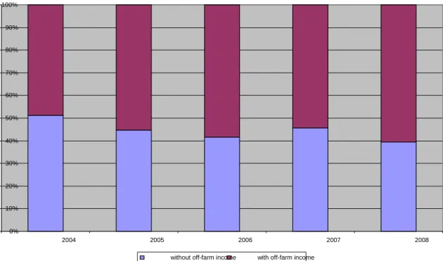
Figure 1. Share of farms with and without off farm income in the Slovenian FADN sample 100% 90% 80% 70% 60% 50% 40% 30% 20% 10% 0% 2007 2004 2005 2006 2008
with off-farm income without off-farm income
Not all analysed Slovenian FADN farms have off-farm sources of income. Out of all number of observations in the FADN sample in the period 2004-2008, there are 40.2% of observations of farms with non-farm income. The percentage of FADN farms with non-farm income varies by individual years, but it tends to increase over the years from 2004 to 2008 (Figure 1). The share of farms with non-farm income varies also by production branches. The percentage of farms with non-farm incomes is above the Slovenian FADN average for milk and other grazing livestock farms, but below this average for wine, livestock using cereals (pigs and poultry), horticulture, field crops, other permanent crops, and mixed farms (Figure 2). This implies that on average more specialised into farm income activates with the lower percentage of non-farm incomes are in Slovenia traditional more labour intensive milk and grazing livestock farms, which can also be situated in more remote hilly areas with less non-farm employment opportunities.
Figure 2. Share of farms with and without off-farm income by production branches with off-farm income
without off-farm income
100% 80% 60% 40% 20% 0%
Field crops Horticulture Livestock using cereals
(pigs and poultry)
Mixed
Wine Other Milk Other grazing total permanent livestock
crops
Table 1 presents descriptive statistics of the FADN data used in the empirical analysis. The non-farm income varies considerable between this kind of farms as can be seen from the comparison of the minimum and maximum values. On average, the Slovenian FADN farms are of the small economic size (18 ESU), but there are also considerable differences between them in terms of ESU and output size, level of intermediate consumption, size of real fixed assets, total utilised agricultural area used, and total labour input at the FADN farm.
Table 1. Summary Statistics, 2004-2008 Variables
Number of
Observations Mean Std. Dev. Minimum Maximum Real output 3358 40010.48 62562.11 -50279.97 2278904 Real intermediate consumption 3358 23814.91 28381.87 290.3001 283065.7 Real fixed assets 3358 300767 563678 532.1267 1.93e+07 Total utilised agricultural area 3358 20.25901 20.3980 0.68 325.62 Total labour input 3358 2.207782 1.7663 0.12 46.08 Off-farm income 1350 0.0232 0.1927 0.000016 7.017 Economic size in ESU 3358 17.998 19.9096 2.005 314.194
Source: Own calculations based on the Slovenian FADN data Empirical results
We present our results in following steps. First, we provide an overview on the SFA estimations. Second, we focus on the stability of SFA scores during analysed period. Finally, we try to explain the TE scores using various estimation methods starting from a simple pooled OLS model, moving to panel models and quantile regressions.
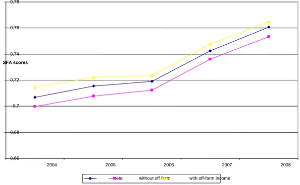
Stochastic frontier analysis (SFA) confirms that the SFA scores have tended to increase for the Slovenian FADN sample of farms, particularly since 2006 (Figure 3). Interestingly, the farms with non-farm incomes on average have experiences higher SFA scores than farms without non-farm income. This might imply that a part of non-farm incomes have been invested into farm activities contributing to their technological advancements over the farms without non farm incomes.
Figure 3. Mean of stochastic frontier analysis scores for the Slovenian FADN farms Mean of SFA 0,78 0,76 0,74 SFA scores 0,72 0,7 0,68 0,66 2004 2005 2006 2007 2008
with off-farm income total without off-farm
The functional specification of the stochastic production frontier was determined by testing the adequacy of the TL specification to the data relative to the more restrictive CD specification. The generalised LR test shows that the TL specification fits the data better than the CD specification.
The variance parameter, γ, which lies between 0 and 1, indicates that technical inefficiency is stochastic and that it is relevant to obtaining an adequate representation of the data. The value of γ picks up the part of the distance to the frontier explained for the inefficiency. In our estimation, the value of the variance parameter γ is around 0.98. That means that the variance of the inefficiency effects is a significant component of the total error term variance and then, farms’ deviations from the optimal behaviour are not only due to random factors. The stochastic frontier is a more appropriate representation than the standard OLS estimation of the production function.
Table2. Stochastic Frontier Time-Varying Decay Inefficiency Model, 2004-2008 Variable Coefficient Constant -2.687 ln x1 -0.632* ln x2 -0.538 ln x3 0.952*** ln x4 0.704*** ½ln 2 1 x 0.098** ½ln 2 2 x 0.218*** ½ln 2 3 x 0.092*** ½ln 2 4 x 0.016 ln x1 ln x2 -0.102*** ln x1 ln x3 -0.016 ln x1 ln x4 0.042 ln x2 ln x3 -0.026 ln x2 ln x4 0.094*** ln x3 ln x4 -0.084*** ln σv -0.102*** Number of observations 3353
Source: Own calculations based on the Slovenian FADN data.
Note: x1 = real total intermediate consumption, x2 = real total fixed assets, x3 = total utilised agricultural area, and x4 = total labour input.
Stochastic frontier time-varying decay inefficiency model indicates a positive and significant association of the stochastic frontier time-varying decay inefficiency in terms of real total output, which is used as the dependent variable, with the traditional agricultural inputs, i.e., total utilised agricultural area and total labour input, respectively. The negative association is found with real total fixed assets, which the regression coefficient is insignificant, and real total intermediary consumption, which is significant, but at 10% significance level. Except for total labour input, all regression coefficients for the square explanatory variables are of a positive sign and significant. The regression coefficients for the interaction effects of the explanatory variables are mixed. A positive and significant association is for the regression coefficient of the interaction effect of the real total fixed assets and total labour input, while of a negative sign and statistically significant is for the regression coefficient of two interaction effects: real total intermediate consumption and real total fixed assets, and total utilised agricultural area and total labour input. These results indicates that more utilised agricultural area and more labour input the farm employs, more inefficient it is, and vice versa for intermediate consumption and to a lesser extent for total fixed assets. The farm inefficiency is mitigated in a combination of intermediate consumption and fixed assets, and agricultural area and labour input, and vice versa for fixed assets and labour input.
Technical efficiency (TE)
First, we present distribution of TE scores using normal density and Kernel density function. As can been seen in Figure 4 the density of distribution of TE scores by the Slovenian FADN farms is asymmetric towards the right hand side of the Kernel density estimate. The pick in the concentration of the Kernel density of TE estimates is around 0.9, and the majority of the Slovenian FADN farms experienced TE scores greater than 0.7. This distribution may imply the problem of heteroscedascity. Moreover, farms with non-farm
income have experienced greater peak in technical efficiency concentration than farms without non-farm income as can be seen from different graph scale and curve distribution. Figure 4. Distribution of technical efficiency scores
0 1 2 3 4 Density 0 .2 .4 .6 .8 1 Technical efficiency Kernel density estimate Normal density
kernel = epanechnikov, bandwidth = 0.0289
Kernel density estimate
0 1 2 3 4 Density 0 .2 .4 .6 .8 1 Technical efficiency
kernel = epanechnikov, bandwidth = 0.0289 total 0 1 2 3 4 Density 0 .2 .4 .6 .8 1 Technical efficiency
kernel = epanechnikov, bandwidth = 0.0308 non farm income
0 1 2 3 Density 0 .2 .4 .6 .8 1 Technical efficiency
kernel = epanechnikov, bandwidth = 0.0371 without non farm income
Table 3. Technical Efficiency Scores and Their Changes, 2004-2008 technical efficiency scores
Number of observations Mean Std. Dev. Minimum Maximum
2004 494 0.706 0.178 0.088 0.960
2005 659 0.715 0.178 0.111 0.964
2006 634 0.719 0.180 0.138 0.967
2007 746 0.742 0.166 0.168 0.971
2008 820 0.760 0.156 0.123 0.973
changes in technical efficiency scores
2005 455 1.038 0.035 1.003 1.271
2006 528 1.038 0.036 1.003 1.2418
2007 566 1.036 0.033 1.003 1.215
2008 680 1.032 0.0288 1.002 1.192
Source: Own calculations based on the Slovenian FADN data.
Second, we present the results of TE scores by the analysed years 2004-2008 (Table 3). Except on average stagnation in TE in 2006, the TE scores tend to increase from year to year, which confirms a pattern of an increase in FADN farm TE. At the same time the gap between the minimum and maximum TE scores by individual farms has been reduced particularly due to a more rapid increase in the TE scores for the least technically efficient FADN farm.
Third, we present the results for the changes in TE scores between the consecutive years. The rate of growth in TE varied between 3.2% and 3.8% in analysed period. The positive rates of growth in TE are also confirmed for the least and particularly for most efficient Slovenian FADN farms. These results confirm a steady and particularly fast growth in TE over time for the most efficient Slovenian FADN farms.
By type of farming, other grazing livestock farms are the least TE (Table 4). Among less TE are also mixed farms and field crops farms. Close to average TE are other permanent crops farms and milk farms. Horticultural farms are found to have the highest TE scores. Among more TE are also wine farms and livestock farms using cereals (pigs and poultry farms). Horticultural farms and livestock farms using cereals (pigs and poultry) experienced also the greatest similarity in TE with the smallest differential between the least minimum and the most maximum TE farms. This differential is particularly large for other grazing livestock farms, field crops farms, other permanent crops farms, and mixed farms.
Table 4. Mean Technical Efficiency Scores by Agricultural Sectors by Type of Farming, 2004-2008
Obs Mean Std. Dev. Min Max
1 Field crops 326 0.680 0.200 0.140 0.955
2 Horticulture 45 0.865 0.079 0.594 0.952
3 Wine 128 0.824 0.144 0.378 0.973
4 Other permanent crops 167 0.751 0.194 0.157 0.964
5 Milk 1220 0.762 0.105 0.248 0.966
6 Other grazing livestock 817 0.598 0.178 0.113 0.951 7 Livestock using cereals (pigs and poultry) 26 0.822 0.105 0.522 0.950
8 Mixed 624 0.661 0.170 0.186 0.946
In addition, Figure 5 presents distribution of TE scores by type of farming. The same scale for each type of farming graph is used to compare directly. While huge differences between types of farming are seen, there are three different patterns in distribution of TE scores by type of farming: first, dispersed pattern in distribution of TE scores with only a slight concentration pick at around 0.8 TE score, which is seen for field crops farms, other grazing livestock farms, and mixed farms. Second, modest concentration pattern in distribution of TE scores is seen for other permanent crops farms. Finally, the greatest concentration in distribution of TE scores at around 0.9 TE score is seen for horticultural farms and livestock farms using cereals (pigs and poultry farms) and to a lesser extent for milk farms and wine farms. These findings are largely consistent with the average TE score with its minimum and maximum values.
Figure 5. Distribution of technical efficiency scores by sectors
0 2 4 6 8 Density 0 .2 .4 .6 .8 1 Technical efficiency
kernel = epanechnikov, bandwidth = 0.0565
Field crops 0 2 4 6 8 Density .2 .4 .6 .8 1 Technical efficiency
kernel = epanechnikov, bandwidth = 0.0250
Horticulture 0 2 4 6 8 Density .4 .6 .8 1 Technical efficiency
kernel = epanechnikov, bandwidth = 0.0413
Wine 0 2 4 6 8 Density 0 .2 .4 .6 .8 1 Technical efficiency
kernel = epanechnikov, bandwidth = 0.0606
Other crops 0 2 4 6 8 Density .2 .4 .6 .8 1 Technical efficiency
kernel = epanechnikov, bandwidth = 0.0185
Milk 0 2 4 6 8 Density 0 .2 .4 .6 .8 1 Technical efficiency
kernel = epanechnikov, bandwidth = 0.0440
Other grazing livestock
0 2 4 6 8 Density .5 .6 .7 .8 .9 1 Technical efficiency
kernel = epanechnikov, bandwidth = 0.0437
Livestock using cereals
0 2 4 6 8 Density .2 .4 .6 .8 1 Technical efficiency
kernel = epanechnikov, bandwidth = 0.0428
Mixed
Panel regression analysis
Preliminary analysis shows that the pooled OLS and panel models are subject to heteroscedasticitiy. Thus, Table 5 presents the results of the panel regression model results of TE with correction of heteroscedasticitiy for the Slovenian FADN sample. The Breusch and Pagan test statistic, which was calculated after random effects estimation, does reject the hypothesis of absence of individual unobserved effects. Both random and fixed effects account for the presence of individual unobserved effects in the model. Although Hausman test suggests that fixed effects estimation has to be preferred, random effect results are also reported. Indeed, fixed effect estimation may lead to imprecise estimates due to the low variations of explanatory variables over time of the (Woolridge, 2002).
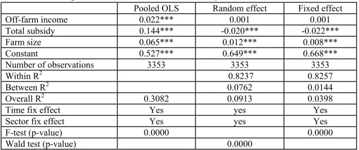
Table 5. Panel Regression Results of Technical Efficiency, 2004-2008
Pooled OLS Random effect Fixed effect
Off-farm income 0.022*** 0.001 0.001 Total subsidy 0.144*** -0.020*** -0.022*** Farm size 0.065*** 0.012*** 0.008*** Constant 0.527*** 0.649*** 0.668*** Number of observations 3353 3353 3353 Within R2 0.8237 0.8257 Between R2 0.0762 0.0144 Overall R2 0.3082 0.0913 0.0398
Time fix effect Yes yes Yes
Sector fix effect Yes yes Yes
F-test (p-value) 0.0000 0.0000
Wald test (p-value) 0.0000
Source: Own calculations based on the Slovenian FADN data.
Note: All estimation procedures account for heteroskedasticity at the firm level and autocorrelation of the error term.
Our special focus is on the association between the farm TE and the non farm income, which is controlled by total subsidies the farm received and the farm economic size. For the farm non farm income we create a dummy variable, which is equal 1 if the farm has the non farm income and 0 otherwise. We found a positive association between the farm TE and the farm non farm income. This spill-over effect of non-farm income on farm TE might be due to relaxation of surplus of farm labour and its remaining more efficient use on the farm due to possible investment in more advanced technology, which in turn provides a higher farm TE. This argument is also in a line with the positive association between the farm TE and total farm subsidies on one hand, and between the farm TE and the farm economic size on the other. More subsidies receive larger farms, which are likely to use subsidies for investment and farm growth that is consistent with their contributions to the improvement in the farm TE. However, these findings hold only for the pooled OLS regression. The results of the random and fixed effect models are mixed. While the regression coefficient for non farm income is of a positive sign, it is insignificant. In these two regression models total subsidies reduce, while farm economic size increases the FADN farm TE. The contradiction results for total subsidies imply that farmers become more convenient on government transfer payments, which distort factor allocation and more likely reduces technical efficiency. In addition to the problem of heteroscedasticitiy, the regression residuals, however, in all cases significantly depart from normal distribution as the Shapiro–Wilk and Shapiro–Francia test results as both reject the null hypothesis of normality distribution at a percentage level. While those slope coefficients may represent a plausible relationship between the farm TE and control variables, the failure to pass miss-specification tests indicates that it is worth going beyond the average tendency and investigating the separate responses of TE to other variables at different quantiles of the technical efficiency.
Quantile regression analysis
Panel regression analysis estimates the relation between the farm TE score as dependent variable and variations in the explanatory variables. It is possible, however, that marginal effects of changes in some of the variables are not equal across the whole distribution of TE scores and the estimated panel regression coefficients may be a poor estimate of the relation between some of the explanatory variables and farm TE score at different quantiles of its
distribution. Quantile regression is a way to overcome this problem, by providing estimates of the regression coefficients at different quantiles of the dependent variable.
With the quantile regressions we test the association between a farm TE and a farm non farming income using control explanatory variables for total subsidies and economic farm size. Figure 6 presents quantile regression estimates and OLS coefficients with confidence interval for explanatory variables with the intercept, which increases with the quantile increases. The average value for the increasing intercept value is a bit more than 0.5 at the quantile less than 0.5. The estimated quantile regression and OLS coefficient with confidence interval for non-farm income experienced first increasing, and then declining patterns with the quantile increases. In the first increasing phase between quantiles 0.1 and 0.5, with the higher farm TE, the stronger is association with non-farm income and the large gap between the quantile regression and OLS coefficient with confidence interval a slightly converges. With the further quantile increases from the average 0.5 quantile, with higher farm TE the weaker is the association with non-farm income, which curves tend to decline with a slightly converging gap between the quantile regression and OLS coefficient confidence intervals. This a roof type curve distribution between farm TE and non-farm income suggests that the least TE efficient farms to a lesser extent experience non-farm income, while over a certain level of farm TE efficiency farms less use non-farm income. Total subsidies took a lower relative scale, including a negative average value since 0.25 quantile and minimum values. They tend to increase between 0.25 and 0.5 quantiles, and after that they on average stabilised. The estimates for economic farm size clearly confirm declining and converging patterns between the quantile regressions and OLS confidence intervals with the quantile increases.
Figure 6. Quantile regression estimates for explanatory variables
0.20 0.40 0.60 0.80 1.00 Intercept .1 .25 .5 .75 .9 Quantile 0.00 0.01 0.02 0.03 0.04 nfarmincome .1 .25 .5 .75 .9 Quantile -0.20 -0.10 0.00 0.10 0.20 total s ubsi d y .1 .25 .5 .75 .9 Quantile 0.00 0.05 0.10 0.15 lnsize .1 .25 .5 .75 .9 Quantile
Table 6 reports the results for a sequence quantile regression estimation for the 0.10, 0.25, 0.50, 0.75 and 0.90 quantiles of the farm TE distribution and tests for equality of coefficients across quantiles were performed. The estimation results confirm that the relation between the Slovenian FADN farm TE and explanatory variables is changing across the whole distribution of the farm TE scores. We found a positive and significant association between the farm TE and the non farm income. The partial regression coefficient for the non farm income a steady decreases between 0.10 quantile and 0.75 quantile, but a slightly increases for the 0.90 quantile of the farm TE distribution. This confirms that sensitivity of the farm TE on the farm off-farm income is different for farms having lower or having higher TE than the median farm TE in the sample of the Slovenian FADN farms. Farms having lower TE scores than the median value (50th percentile) show a significantly larger sensitivity to non farm income. Interestingly, the Wald test confirms the null hypothesis of equality of the coefficient across quantiles for the non farm income. We control the non farm income explanatory role in quantile regression by total subsidies that are received by a farm and by farm economic size, and by time fix effect and sector fix effect. The association between the farm TE and the farm economic size is of a positive sign and significant for the each quantiles. The absolute size of the partial regression coefficient declines with the quantile increases. This implies that the increase in farm economic size improves farm TE more for smaller than larger farms vis-à-vis the median value (50th percentile). In general, .larger farms are more efficient, but this farm size effect decreases with increasing farm size. The Wald test confirms statistical significant association between the farm TE and farm economic size across quantiles. The association between the farm TE and total subsidies is of a positive sign, but only significant for the median 0.50 quantile. The statistical insignificant association between the farm TE and total subsidies by quantiles is also confirmed by the Wald test. Table 6. Quantile Regression of Technical Efficiency, 2004-2008
Q10 Q25 Q50 q75 q90 Wald test (p-value)
Off-farm income 0.028*** 0.023*** 0.021*** 0.015*** 0.019*** 0.6494 Total subsidies 0.148 0.108 0.068* 0.021 0.015 0.6357 Economic size 0.098*** 0.089*** 0.061*** 0.034*** 0.020*** 0.0000 Constant 0.215*** 0.361*** 0.588*** 0.742*** 0.843*** 0.0000
Time fix effect Yes yes Yes yes yes
Sector fix effect Yes yes Yes yes yes
N 3314 3314 3314 3314 3314
Pseudo R2 0.2799 0.2557 0.1859 0.1127 0.0699
Source: Own calculations based on the Slovenian FADN data.
Note: Level of significance: * p<0.1; ** p<0.05; *** p<0.01 based on bootstrapped standard errors with 1000 replications. Wald test of equality of the coefficient from quantile regression when: q = 0.10, q = 0.25, q = 0.50, q = 0.75, and q = 0.90 (probability).
Conclusions
Slovenian agricultural farm structures are typical by off-farm employment and off-farm incomes. While on average the Slovenian farms are of relatively a small size, they are largely engaged in off-farm employment. This holds also for the Slovenian FADN farms, which on average are larger and more economically vital than the average Slovenian farms. More than 40% of the Slovenian FADN farms have the off-farm income sources.
We confirm that the off-farm income improves the FADN farm TE, which implies spill-over effect’s spread of the off-farm income on farm TE. On one hand the off-farm income provides cash flow into a farm, which can be also invested in farm’s technological advancements, which improve farm TE. On the other hand the off-farm employment, which is associated with the off-farm incomes, relaxes possible farm labour surpluses outside the main seasonal work, which in turn gives to farm an opportunity that a maximum possible farm output at given technology is achieved with less of farm labour employment. Looking dynamically over time, average farm TE scores have increased and the off-farm income is found to have a positive role in this farm TE improvements.
Both the panel regression models and the quantile regressions of TE confirm the positive association between farm TE and the off-farm income. This further reinforces farm managerial and policy implications on the positive role of off-farm employment and off-farm income, when farms on average are of relatively a small technical operational and economic size giving them to relax a surplus of labour and at the same time giving them an opportunity for additional farm households’ incomes that can be invested in farm advancements, farm growth, and farm survival, as well as they can improve economic well being of the farm households’ members. The off-farm income is important for farm TE by different quantiles, a bit more important for smaller than for greater quantiles. This is further reinforced by the positive association between the farm TE and the economic farm size implying the importance of economic farm size growth, particularly for a smaller quantiles of farms. The association of farm TE and farm subsidies is found to be mixed depending on the estimation procedure: it is of a positive sign in the pooled OLS regression, but of a negative sign in the random and fixed effect panel models. Moreover, the quantile regression of TE suggests a positive association between farm TE and farm subsidies, which is significant only for the median value (50th percentile) quantile. This implies that farm subsidies do not necessary improve farm TE and thus their targeting objectives should be clearly defined within the reform of Common Agricultural Policy and particularly within implementation objectives and measures.
Literature
Ahituv, A. and Kimhi, A. 'Simultaneous estimation of work choices and the level of farm activity using panel data', European Review of Agricultural Economics, Vol. 33, (2006) pp. 49–71.
Ahearn, M.C., El-Osta, H. and Dewbre, J. 'The impact of coupled and decoupled government subsidies on off-farm labor participation of U.S. farm operators', American Journal of Agricultural Economics, Vol. 88, (2006) pp. 393–408.
Aigner, D., Lovell, K. and Schmidt, P. ‘Formulation and estimation of stochastic frontier production function models’, Journal of Econometrics, Vol. 6, (1977) pp. 21–37. Bagi, F.S. 'Stochastic frontier production function and farm-level technical efficiency of full-time and part-time farms in west Tennessee', North Central Journal of Agricultural Economics, Vol. 6, (1984) pp. 48–55.
Battese, G.E. and Coelli, T.J. ‘A model for technical inefficiency effects in a stochastic frontier production function for panel data’, Empirical Economics, Vol. 20, (1995) pp. 325–332.
Benjamin, C. and Kimhi, A. 'Farm work, off-farm work, and the hired labour: estimating a discrete-choice model of French farm couples’ labour decisions', European Review of Agricultural Economics, Vol. 33, (2006) pp. 149–171.
Bojnec, Š. and Dries, L. ‘Causes of changes in agricultural employment in Slovenia: evidence from micro-data’, Journal of Agricultural Economics, Vol. 56(3), (2005) pp. 399–
416.Bojnec, Š. and Latruffe, L. ‘Measures of farm business efficiency’, Industrial Management & Data Systems, Vol. 108, (2008) pp. 258–270.
Bojnec, Š. and Latruffe, L. ‘Determinants of technical efficiency of Slovenian farms’, Post-Communist Economies, Vol. 21, (2009a) pp. 117–124.
Bojnec, Š. and Latruffe, L. ‘Productivity change in Slovenian agriculture during the transition: a comparison of production branches’, Ekonomický Časopis, Vol. 57, (2009b) pp. 327–343.
Brümmer, B. ‘Estimating confidence intervals for technical efficiency: the case of private farms in Slovenia’, European Review of Agricultural Economics, Vol. 28, (2001) pp. 285– 306.
Buchinsky, M. ‘Recent advances in quantile regression models: a practical guide for empirical research’, Journal of Human Resources, Vol. 33, (1998) pp. 88–126.
Chavas, J.P., Petrie, R. and Roth, M. 'Farm household production efficiency: evidence from the Gambia', American Journal of Agricultural Econonomics, Vol. 87, (2005) pp. 160–179. de Janvry, A. and Sadoulet, E. 'Income strategies among rural households in Mexico: the Role
of off-farm activities', World Development, Vol. 29, (2001) pp. 467–480.
Goodwin, B.K. and Mishra, A.K. 'Farming efficiency and the determinants of multiple job holding by farm operators', American Journal of Agricultural Economics, Vol. 86, (2004) pp. 722–729.
Gorton, M. and Davidova, S. ‘Farm productivity and efficiency in the CEE applicant countries: a synthesis of results’, Agricultural Economics, Vol. 30, (2004) pp. 1–16.
Hennessy, T.C. and Rehman, T. 'Assessing the impact of the “decoupling” reform on the Common Agricultural Policy on Irish farmers’ off-farm labour market participation decisions', Journal of Agricultural Economics, Vol. 59, (2008) pp. 41–56.
Hertz, T. ‘The effect of nonfarm income on investment in Bulgarian family farming’, Agricultural Economics, Vol. 40(2), (2009) pp. 161–176.
Huffman, W.E. 'Farm and off-farm work decisions: the role of human capital', Review of Economics and Statistics, Vol. 62, (1980) pp. 14–23.
Lass, D., Findeis, J. and Hallberg, M. 'Off-farm employment decisions by Massachusetts farm households', Northern Journal of Agricultural Resource Economics, Vol. 18, (1989) pp. 149–159.
Lien, G., Flaten, O., Jervell, A.M., Ebbesvik, M., Koesling, M. and Valle, P.S. 'Management and risk characteristics of part-time and full-time farmers in Norway', Review of Agricultural Economics, Vol. 28, (2006) pp. 111–131.
Lien, G., Kumbhakar, S.C. and Hardaker, J.B. ‘Determinants of off-farm work and its effects on farm performance: the case of Norwegian grain farmers', Agricultural Economics, Vol. 41(6), (2010) pp. 577-586.Koenker, R. and Bassett, G. ‘Regression quantiles’, Econometrica, Vol. 46, (1978) pp. 33–50.
Koenker, R. and Hallock, K.F. ‘Quantile regression’, Journal of Economic Perspectives, Vol. 15, (2001) pp. 143–156.
Meeusen, W. and van den Broeck, J. ‘Efficiency estimation from Cobb-Douglas production functions with composed error’, International Economic Review, Vol. 18, (1977) pp. 435– 444.
Mishra, A.K. and Goodwin, B.K. 'Farm income variability and the supply of off-farm labor', American Journal of Agricultural Economics, Vol. 79, (1997) pp. 880–887.
Pfeiffer, L., López-Fledman, A. and Taylor, J.E. 'Is off-farm income reforming the farm? Evidence from Mexico', Agricultural Economics, Vol. 40, (2009) pp. 125–138.
Rizov, M., Gavrilescu, D., Gow, H., Mathijs, E. and Swinnen, J.F.M. ‘Transition and enterprise restructuring: the development of individual farming in Romania’, World Development, Vol. 29(7), (2001) pp. 1257–1274.Rizov, M. and Swinnen, J.F.M. ‘Human
capital, market imperfections, and labor reallocation in transition’, Journal of Comparative Economics, Vol. 32(4), (2004) pp. 745–774.
Serra, T., Goodwin, B.K. and Featherstone, A.M. 'Agricultural policy reform and off-farm labour decisions', Journal of Agricultural Economics, Vol. 56, (2005) pp. 271–285.
Singh, S.P. and Williamson, Jr., H. 'Part-time farming: productivity and some implications of off-farm work by farmers', Southern Journal of Agricultural Economics, Vol. 6, (1981) pp. 61–67.
Weersink, A., Nicholson, C. and Weerhewa, J. 'Multiple job holdings among dairy families in New York and Ontario', Agricultural Economics, Vol. 18, (1998) pp. 127–143.
Woldehanna, T., Oude Lansink, A. and Peerlings, J. 'Off-farm work decisions on Dutch cash crop farms and the 1997 and Agenda 2000 CAP reforms', Agricultural Economics, Vol. 22, 2000 pp. 163–171.
Woolridge, J.M. Econometric Analysis of Cross Section and Panel Data (Cambridge: The MIT Press, 2002).