Distributed traffic
forecast-ing usforecast-ing Apache Spark
Boufidis Neofytos
SID: 3308170003SCHOOL OF SCIENCE & TECHNOLOGY
A thesis submitted for the degree of
Master of Science (MSc) in Data Science
DECEMBER 2018
Distributed traffic forecasting
using Apache Spark
Boufidis Neofytos
SID: 3308170003Supervisor: Prof. Papadopoulos Apostolos
SCHOOL OF SCIENCE & TECHNOLOGY
A thesis submitted for the degree of
Master of Science (MSc) in Data Science
DECEMBER 2018
Abstract
This dissertation was written as a part of the MSc in Data Science at the International Hellenic University. The exploding volume of available data in recent years render the development of distributed algorithms vital for most scientific fields, including Transpor-tation and Intelligent Transport Systems. This thesis investigates the use of big data tech-nologies for enhancing urban transportation and planning. A sophisticated traffic fore-casting model is developed and tested utilizing a large-scale, real-world dataset produced by GPS sensors on a taxi fleet (i.e., floating car data) in the area of Thessaloniki, Greece. The model implementation, including parts of the data preprocessing steps, are imple-mented in PySpark, the Python API of Spark distributed programming language.
At this point I would like to thank my supervisor, professor Apostolos Papadopoulos, for his support and guidance throughout my thesis completion. I would also like to thank my colleagues Josep Maria Salanova Grau and Panagiotis Tzenos, who shared invaluable insights from the field of Transportation and also agreed to contribute the data that ena-bled the development and validation of the algorithms and models. Without the afore-mentioned scientists’ passionate participation and input, this master’s dissertation could not have been successfully conducted.
Boufidis Neofytos 6 December 2018
Contents
ABSTRACT ... III CONTENTS ... V
1 INTRODUCTION ... 1
2 LITERATURE REVIEW ... 3
2.1 TRADITIONAL TRANSPORTATION RESEARCH DATA SOURCES ... 3
2.2 FLOATING CAR DATA (FCD) ... 3
2.3 FCD APPLICATIONS ... 4
2.3.1 Traffic Prediction ... 4
2.3.2 Anomaly Detection in Road Networks ... 7
2.3.3 Driver Ranking and Passenger/Taxi-Finding Strategies ... 9
2.3.4 Transportation Optimization and Planning ... 9
2.3.5 Environmental Studies ... 11
2.3.6 Social Activities ... 11
3 BIG DATA ... 13
3.1 CHARACTERISTICS ... 13
3.2 CHALLENGES AND THE CLOUD ... 13
3.3 METHODS AND TOOLS FOR ANALYSIS ... 14
3.3.1 Parallel computing... 14
3.3.2 Hadoop ... 15
3.3.3 Spark ... 15
4 METHODOLOGY ... 17
4.1 THE DATASETS ... 17
4.1.1 The Floating Car Dataset ... 17
4.1.2 The digitized road network of Thessaloniki ... 18
4.2 DATA PREPROCESSING ... 19
4.3.1 Point to link distance ... 22
4.3.2 Map-matching algorithm ... 23
4.4 TIME SERIES TRANSFORMATION ... 25
4.5 DATA LIMITATIONS AND FORMULATION OF THE PREDICTIVE ALGORITHM ... 26
4.6 FEATURE EXTRACTION ... 27
5 RESULTS ... 29
5.1 MACHINE LEARNING ALGORITHMS ... 29
5.1.1 Multiple Linear Regression... 29
5.1.2 Random Forest Regression ... 30
5.1.3 Gradient Boosting Trees Regression ... 30
5.2 EVALUATION TECHNIQUES AND METRICS ... 30
5.2.1 Mean of squared errors ... 31
5.2.2 Root mean of square errors ... 31
5.2.3 Mean of absolute errors ... 31
5.3 MODEL TUNING ... 31 5.4 FORECASTING RESULTS ... 32 6 CONCLUSION ... 35 7 FUTURE PROSPECTS ... 37 8 BIBLIOGRAPHY ... 39 APPENDIX A ... 47 APPENDIX B ... 48 APPENDIX C ... 49 APPENDIX D ... 50
1
Introduction
During the last decade, advances in technology have resulted in an exponential in-crease of the data generation rate. Data growth has revolutionized the way innovative companies produce, operate, manage their assets and plan. The scientific community identified the birth and significance of Big Data since 2000 and Doug Laney introduced the three Big Data V’s, data volume, velocity, variety in 2001 [1]. Ten years later scien-tists and industry consider another four characteristics, data validity, veracity, value, vis-ibility as equally important.
Nowadays, companies dash to adopt Big Data technologies, such as in memory tech-nologies, to cope with the huge volume of data and gain Business Intelligence, enabling them to offer products and services of the highest quality and standards. Examples are endless, from personalized advertisement and recommendation systems, to Artificial In-telligence applications like fully or semi-autonomous vehicles, to clever, humanlike chat-bots like Apple’s Siri and Microsoft’s Cortana.
In the field of Transportation, the latest scientific discoveries are complemented with big data tools that have empowered the development of state-of-the-art Intelligent Transport Systems (ITS) that fuse data from different sources and utilize sophisticated data analytics tools and recent scientific discoveries. This dissertation will focus on de-veloping a tool for processing and analyzing transportation data generated by GPS trans-mitters installed on vehicles. Such datasets are known in bibliography as Floating Car Data (FCD) and have been used extensively for numerous applications including moni-toring and optimizing road networks, vehicle routing, outlier and anomaly detection, mo-bility pattern identification and traffic forecasting.
The raw data of this project are generated from a vehicle fleet that consists of approx-imately half the taxis operating in the region of Thessaloniki, Greece. The association that manages this fleet of taxis (TaxiWay) has a long-term collaboration agreement with the Center for Research and Technology Hellas – Hellenic Institute of Transport (CERTH – HIT), which has agreed to provide access to part of the database, only for the purpose of this research study.
The development of the traffic prediction model for this project contains a number of complicated procedures, since the road network of Thessaloniki has to be constructed and viewed as a mathematical multi-directed graph while raw data has to be matched on the corresponding road segment according to their longitude and latitude values, which con-tain cercon-tain amount of inaccuracy. The aforementioned analysis will be implemented us-ing the programmus-ing languages Python and PySpark, the Python API of Spark, which allows for parallel computations and processing of huge datasets with great performance.
The structure of this dissertation is as follows:
Chapter 2 includes an exhaustive literature review and state-of-the-art definition on the concepts of geospatial and floating car data (FCD) processing and analysis, FCD ap-plications and road traffic forecasting, and justifies the novelty of our proposed approach and solution.
Chapter 3 thoroughly describes the buzz term ‘Big Data’ and presents state-of-the-art Big-Data technologies
Chapter 4 comprehensively explains the problem definition and the adopted meth-odology within the project’s scope.
Chapter 5 presents the most significant findings and conclusions extracted from this thesis.
Chapter 6 summarizes the most important findings and lessons learned during the implementation of this project.
Chapter 7 includes the author’s opinion for further improvements and advancements
2
Literature Review
In this section the results of an in-depth literature review of the most recent scientific publications are presented. The review covers all scientific topics relevant to this thesis, from geospatial and floating car data (FCD) processing and analysis methodologies to road network traffic prediction techniques. Furthermore, comparisons between the litera-ture and the present study are drawn.
2.1 Traditional Transportation Research Data
Sources
The generation of huge amounts of traffic related, GPS data has steered research to new data driven models and applications. Early studies on human activity and mobility pat-terns and Transportation management have been based on survey and questionnaire data, which come in limited quantity, are not automatically recorded and thus expensive, can-not be processed in real time and thus have limited value when the task is traffic optimi-zation [2]. The following years, road side equipment (stationary cameras and detectors placed at crucial road network points) captured data about traffic volume and vehicle speed. However, the system’s imperfect accuracy, high installation and maintenance cost, and restricted road network coverage limit its potential. As a result, such infrastructure is mainly utilized by authorities for traditional Transportation network monitoring [3]. Cur-rent studies and applications concerned with dynamic traffic management, optimization and forecasting have proved FCD as the most valuable data source [3] [4] [5]. In this study, we have utilized FCD from vehicles in the region of Thessaloniki, Greece.
2.2 Floating Car Data (FCD)
FCD is currently the main source of real time information about traffic condition on road networks [6], as data are generated and recorded passively in a fully automated procedure by driving vehicles. It is a simple and relatively cheap technology [7], since most vehicle fleets nowadays have already incorporated monitoring systems that include in-vehicle GPS transmitters. The sensor can even be a modern smart device, like the driver’s smartphone or a tablet used in the vehicle for navigation purposes. In the general case, the sensor transmits real time data to a server, which then stores them in a database. Other
devices save data in a micro-SD memory card that periodically connects physically or with a wireless connection to a database. GPS signals commonly include information about:
• geolocation of the vehicle, reporting the coordinates (longitude and latitude)
• timestamp
• vehicle id (in the case when a service monitors more than one vehicle)
• speed measure and speed orientation
2.3 FCD Applications
The scope of scientific research utilizing FCD is vast. It concerns Transportation topics like traffic prediction, Transportation network optimization and planning, and anomaly detection in road networks. Furthermore, FCD studies have produced significant results related to other fields like Social and Environmental Sciences.
2.3.1 Traffic Prediction
Traffic prediction algorithms are at the heart of numerous Intelligent Transport Systems developed by scientists attempting to cope up with the increasing number of vehicles on the existing road network and infrastructure. The high value and increasing availability of FCD have paved the way to an abundance of literature available for the topic of traffic prediction, and in the following paragraphs the most significant and modern scientific publications utilizing FCD are reviewed.
According to a systematic literature review on the topic of short-term real-time traffic prediction methods by Barros et al. [5], the main characteristics that differentiate studies of the field and the predictive models they propose are:
i. Data collection and processing: Data may arrive in real-time and be processed online, or historical data may be processed offline
ii. Prediction targets and granularity: Some studies forecast traffic in high detail, breaking down the road network to small segments and forecast the traffic at each street, while others adopt more coarse-grained approaches decomposing a region
Figure 1: Grid decomposition (left), traces from 20 taxis (center) and digitized road network (right) for the city of Hangzhou, China.
iii. Evaluation prediction metrics: The different models are tested, and their perfor-mance is reported using a number of metrics (e.g. accuracy and precision for clas-sification and mean average precision error for regression)
iv. Methodology and approach: Some approaches are model-driven and utilize sim-ulations of the road network. Others are data-driven and most commonly exploit well known techniques from Statistics (e.g. Auto-Regressive Integrated Moving Average methods) and Machine-Learning (e.g. Artificial Neural Networks).
Our proposed model is data-driven, built for both historical and online data pro-cessing, considering a digitized road network of Thessaloniki. Multiple metrics are cal-culated in order to evaluate our model’s performance.
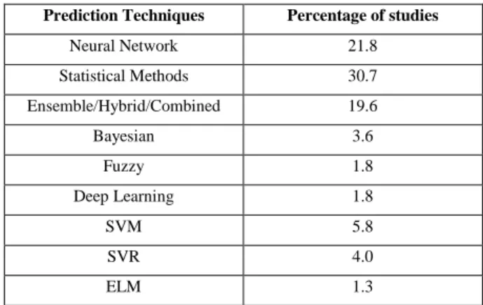
According to the most recent literature review conducted on traffic prediction for ITS [8], the majority of scientists and studies utilize Statistical methods for predictions [Fig-ure 1]. However, this review is conducted on studies which use heterogeneous data sources beyond FCD, and also states that statistical approaches are mainly used for time-series analysis, while neural networks have showed more accurate performance with real-world data, since traffic data is nonlinear.
Table 1: Comparison of percentage of studies conducted on predictive techniques for ITS.
Prediction Techniques Percentage of studies
Neural Network 21.8 Statistical Methods 30.7 Ensemble/Hybrid/Combined 19.6 Bayesian 3.6 Fuzzy 1.8 Deep Learning 1.8 SVM 5.8 SVR 4.0 ELM 1.3
k-NN 4.0 Hidden Markov Models 1.3 Kalman Filter 2.2 Stochastic Process 1.3 Random Forest 0.9
The same study also reveals that the most commonly used features for predictions are speed, traffic flow (i.e. number of cars per time unit) and traffic volume (i.e. number of cars). Obviously, traffic flow and volume are features only available when road side equipment (e.g. cameras) are used for recording traffic data. When working with FCD, a researcher can deduce those numbers taking into consideration the percentage of vehicles contributing to the FCD, but the error could render such estimations useless. Surprisingly, only 3.3% of studies include weather data in the models, which according to the authors suggest the high unavailability of open, accurate and fine-grained weather data for many regions. Regarding performance evaluation measures, root mean squared error (RMSE) and mean absolute percentage error (MAPE) are the most commonly used. Unfortunately, the review did not present a detailed analysis of the nature of datasets used in the reviewed papers, however it states that privately owned datasets, including spatiotemporal GPS data are utilized in 66.2% of studies.
Fabritiis et al. [9] developed a system for online, short time (15 and 30 minute) road speed predictions on Rome’s ring road (GRA-Grande Raccordo Anulare). Two models were tested and compared. The first was an artificial neural network and the results sug-gested that it was the best in terms of prediction performance. It was used in a regression approach, with good prediction accuracy and generalization abilities, achieving a MAPE of 2%-8% for 15 min. predictions and 3%-16% for 30 min. predictions. The RMSE varied between 2 and 7 km/h. The second model was a classification approach utilizing Pattern-Matching and achieved a 18.7% misclassification error.
A neural network (NN) also demonstrates its capabilities in [10], earning its creators the 5th place in the international competition held in 2010 by Tom-Tom, a company pro-ducing automotive navigation systems. In order for the team to reach the best perfor-mance, several different NN architectures were tested, using different combination of in-put features, training methods and epochs. The best performing NN’s architecture was simple, with two input units, utilizing the average velocities and number of GPS pulses
training technique but adds a heuristic that decreases the probability that training will converge to a local minimum. The lowest RMSE achieved is 9.15.
A more recent research paper examines the capabilities of deeper ANN for traffic predictions considering a classification approach [11]. The algorithms are created using Python and its most widely used scientific libraries for data science, like Pandas for data processing and TensorFlow for developing the deep neural networks. The NN consists of 3 hidden layers, with 40, 50 and 40 neurons respectively and achieved a 99% prediction accuracy.
To the best of the authors knowledge, there is only one traffic prediction study utiliz-ing FCD from the city of Thessaloniki [4]. It investigates the problem of short-term speed prediction on street level and compares the capabilities of a statistical ARIMA model to an artificial neural network. Several tests are run, with a wide range of parameters values for the ARIMA and different structures for the NN, but also different prediction time windows, from 5 to 60 minutes. In addition, the problem is also addressed as a multilabel classification, categorizing roads as red (heavy congestion), orange (light congestion) and green (no congestion). However, the whole analysis is somewhat limited, as it is only using traditional technologies for data processing and analysis, without utilization of the most modern big data tools like Spark or Hadoop.
Theodorou et. al. [12] propose a hybrid data-driven model able to adapt to the network state, using an SVM model to classify traffic conditions as typical (normal) or atypical. The short-term traffic predictions are issued by an Auto-Regressive Integrated Moving Average (ARIMA) or k-Nearest Neighbors model, in the typical and atypical case respec-tively.
Sunderrajan et al. [13] focused on the minimum penetration of FCD for accurate traf-fic status estimations, and results suggest that reliable predictions can be produced if at least 5% of road vehicles are monitored and contribute to the FCD.
2.3.2 Anomaly Detection in Road Networks
In general, anomaly (or outlier) detection refers to the identification of observations, items or events that significantly differ from most other data. Depending on the nature of the dataset and the definition of proximity or similarity amongst data points, anomaly detec-tion can be defined in various ways. Network anomaly detecdetec-tion has been widely studied
and researched in IP networks and is mainly related to network performance problems, failures and security [14]. In road networks, studies mainly focus on detecting anomalies of two types, in traffic and trajectories [15].
A traffic outlier is considered to be a state during which the traffic statistics (travelling speeds, flows etc.) suddenly and intensively change for all or part of the road network. A highly accurate approach is proposed in [16], where normal traffic flows are established for each origin-destination area from historical data and are compared to current obser-vations and traffic flows. The system managed to identify 3 out of 4 situations of actual abnormal situations that were reported by the traffic administrative department in the city of Harbin, China. The proposed system in [17] integrates FCD with data from WeiBo, a Twitter-like social networking site in China. In short, when an anomaly is detected, the algorithm detects the geographical area it affects and extracts posts from the affected area at that particular timeframe. Afterwards, text mining methods are applied on posts and the top terms identified in the posts are reported. The algorithm was tested on two abnor-mal situations and it correctly identified the abnorabnor-mal situation but also the cause, which was a traffic accident and a wedding respectively. Another approach constructs outlier causality trees and is tested and validate with FCD from Beijing, China, and scales almost linearly as the number of outliers to be detected increases, which implies that such an application could work online with data streams [18].
A trajectory can be classified as anomalous if it deviates significantly from past tra-jectories with similar origin and destination in historical data. A proposed algorithm for identifying anomalous trajectories compares the actual distance covered by a vehicle to the shortest network path between the origin and destination nodes. A threshold value for the distance difference is applied and larger values indicate anomalies [19]. Another al-gorithm, called Isolation-Based Anomalous Trajectory (iBAT), is proposed in [20] and successfully detects over 90% of abnormal taxi trajectories achieving a false alarm rate of less than 2%. The same authors have also proposed an updated version of this algo-rithm, iBOAT, that is able to operate online [21]. Tools for anomalous trajectory detection utilizing FCD have been extensively used for uncovering fraudulent trips and routes by taxi drivers [Figure 2]. The levels of accuracy of results [22] [23] reveal the high potential of such tools in a taxi business intelligence platform.
Figure 2: Normal (green) and fraudulent (orange) taxi trips from A to B
2.3.3 Driver Ranking and Passenger/Taxi-Finding Strategies
FCD processing has provided scientists with more tools and techniques for detecting driver characteristics beyond fraudulent taxi trips. A lot of different measures for ranking taxi drivers have been proposed, in an attempt to discover the common attributes and habits along the best drivers [24]. The most common measures calculate driver’s income per working hour and ratio of occupied taxi time. The highest scoring drivers according to those criteria are found to usually choose the fastest routes to their destination, taking into consideration existing traffic conditions, in order to complete the trip and seek for new passengers as soon as possible. Liu et al. [25] conducted further statistical analysis using k-means clustering and revealed that most highly ranked drivers, according to their income, choose similar spatiotemporal places for looking and picking passengers.
Yuan et al. [26], [27] provide taxi drivers with a pick-up location recommendation system. They extract taxi waiting locations from the GPS points and calculate the proba-bility of picking up a passenger as a function of time and location, which is either a taxi-stop or just a road segment.
2.3.4 Transportation Optimization and Planning
The performance of a road network can be improved by rerouting vehicles based on actual traffic conditions inferred from real time FCD processing. Vehicle to infrastructure com-munication protocols have been developed for optimizing traffic flows, and smart adap-tive traffic lights is considered a promising technological innovation towards smart cities and sustainable mobility. In [28], an implementation of a dynamic traffic lights regulation system is presented, which is based on FCD that are transmitted to a unified control center in real time. It is estimated that in order for the adaptive traffic lights to operate efficiently with equal priority to road users, 35% of vehicles have to be connected to the control
center, which is a viable target and drivers are expected to contribute to such systems in the future, as the system will provide valuable services in return. Another case study in Amsterdam shows that the total delay time from traffic congestion might be reduced up to 3.4% for 10% penetration rate of FCD [29]. Τhis time savings are equivalent to about 15m. Euros if monetarized.
A very important research topic in Transportation is the identification of mobility patterns. A usual approach is the definition of origin-destination (O-D) hotspots. O-D matrix computation is a complex task as traffic flows and patterns change dynamically through time, as a function of numerous parameters. In [30], a method for inferring an O-D matrix for Shanghai, China is proposed. It processes FCO-D from taxis to extract trip start and end points, clusters them with the DBSCAN algorithm fusing with point of interest data from Open Street Maps project. Results are easy to interpret with visualizations gen-erated by a web-based application.
Another research based on FCD from probe vehicles proposes an estimation model for on-street parking search time that is tested in Rome, Italy [7]. A method for distin-guishing the final part of a trip when the driver searches a parking spot is presented, and the predictive model can be integrated either in on-line tools for dynamic vehicle routing or off-line research and applications for planning purposes.
Towards the shift to green cities and eco-friendly vehicles, a recent study leverages FCD for smart mobility cities planning [31]. It re-constructs actual trips from a Free-Floating Car Sharing System (FFCS), where customers use available cars freely within the city’s limits. The study analyses the trips and customer behavior and needs for a period of 2 months in the city of Turin, Italy in order to simulate and validate the feasibility of a car sharing system with electric vehicles. It is found that in Turin, a city with approx. 1 million inhabitants, 300 electric vehicles and 15 charging stations would constitute a FFCS solution with the ability to auto-sustain itself.
In another project, FCD reveal the consequences of alternating weather conditions to the road network and vehicle speeds [32]. It is found that during peak times and night, travelling speeds in the city of Beijing might decrease up to 15% and 10% respectively. Furthermore, an effective speed prediction model under different weather conditions is developed.
2.3.5 Environmental Studies
FCD are also utilized in analysis of current or future vehicle pollutant emissions and en-ergy demand, due to their high spatiotemporal resolution. Shaojun et al. utilized data from multiple Intelligent Transportation Systems, mainly composed of FCD, to develop a high-resolution emission inventory for vehicles in Nanjing, China [33]. In a study from Liberto et al. [34], scientists confirm the need of vehicle electrification for achieving sustainable mobility goals by modelling data from Rome, Italy. In detail, it is calculated that by 2025, 10% of private vehicles and 30% of public transport vehicles should use electricity, while the extra amount of electric energy is estimated to 460GWh.
Another study focuses on vehicle fuel consumption. The most crucial parameters cor-related with it are investigated through exploratory data analysis, and an Artificial Neural Network approach is proposed as a capable algorithm for estimating vehicle consumption with high accuracy [35].
2.3.6 Social Activities
In [36], the authors examine the correlation between the physical and digital world in Thessaloniki, Greece, by fusing FCD with data from social networking websites and prove the strength of the relation between social activity and travel patterns, mainly dur-ing the afternoon and night hours, when individuals are more active on social media plat-forms. Another application utilizes FCD and implements ensemble machine learning al-gorithms to establish a trip purpose predictive model [37]. The survey took place in Swit-zerland and the algorithm achieved an accuracy of up to 85%.
In a related study, GPS data streams are processed for activity identification. The pro-duced algorithms are tested on real-world large-scale benchmark datasets, and work and other activities are correctly predicted in 85% and 87% of the cases respectively [2].
Another study with impressive results has been conducted with FCD from the city of Hangzhou, China, where scientists build a model that classifies trips based on their pur-pose [38]. The three categories the paper considers are trips to a) scenic spots, which show very different patterns between holidays and weekdays and have much more passengers in holiday than weekdays, b) trips to train and/or coach stations, where passenger get-on/off peaks occur in uncommon time points with insignificant differentiations among workdays and weekdays and c) entertainment districts, which present similar statistics to
scenic posts but decreased variance between visitor amount peaks and troughs. The method achieves an accuracy higher than 94%.
3
Big Data
In this section the term Big Data is explained, along with the most efficient, state-of-the-art software and techniques for Big Data management and processing.
3.1 Characteristics
As the daily production of data increases steeply, the volume of available data is explod-ing. “Big Data” is an abstract term used to describe massive collections of structured or unstructured data, with a volume so enormous that renders traditional databases and soft-ware for processing prohibited. In 2010, Apache Hadoop defined big data as “datasets which could not be captured, managed, and processed by general computers within an acceptable scope”. The conventional Relational Database Management Systems (RDBMS) cannot cope with big data, as a result of their three main characteristics: vol-ume, velocity and variety [39].
• Data volume refers to the vast size of data. Big data are characterized by huge volume. A bank, for example, might need to process and analyze several gigabytes of customer data on a daily basis.
• Data velocity refers to the update rate of data. Some years ago, yesterday’s data were considered fresh and valuable. Newspapers still follow that logic. Today the end user is interested in the most updated news and wants real-time access to newly generated content, just as a bank wants real time data processing in order to detect fraudulent transactions.
• Data Variety refers to the heterogeneous nature of available data, which can be in numerous different formats, like databases, csv files, text files, multimedia etc.
3.2 Challenges and the Cloud
Companies and stakeholders need to harvest big data in the most efficient way, in terms of time and monetary costs, to extract useful, previously unknown knowledge, insights and business intelligence [40]. However, processing big data is a highly complicated procedure. The vast volume, high velocity and diversity of datasets that have to be
analyzed pose hurdles by no means trivial to overcome. The main difficulties are often lack of human experts and infrastructure, since big data require more resources than just one machine for processing. In this context, individuals and organizations can nowadays take advantage of cloud technologies and services for big data analysis, getting network access to computing resources and/or software, provided by outside entities. Those services are classified as platform (PaaS), software (SaaS), infrastructure (IaaS) or hardware (HaaS) as a service [41].
3.3 Methods and Tools for Analysis
Chen et al. [39] identify that the traditional data analysis methods that can be also applied on big data are cluster analysis, factor analysis, correlation analysis, regression analysis, A/B testing, statistical analysis and data mining algorithms, and also state that pure big data analytic methods and tools include Bloom filters, hashing, indexing, Trie trees and mainly parallel computing.
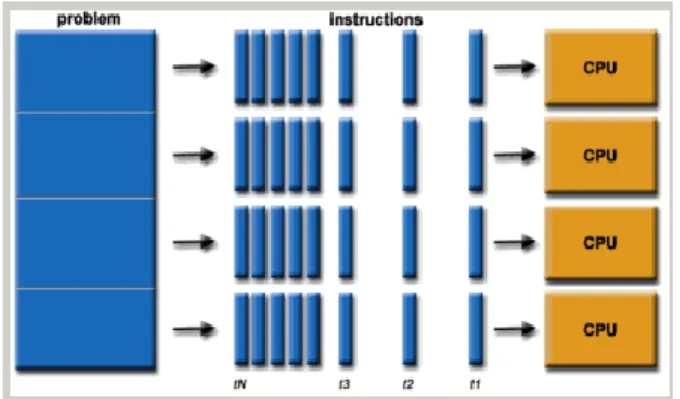
3.3.1 Parallel computing
Parallel computing is a computation paradigm in which the execution of many calculations or processes occur simultaneously [Figure 3], utilizing a number of different processors [42]. Nowadays, the most widely used open source environments for developing distributed algorithms are Hadoop and Spark.
Figure 3: A parallel computing example. The computational problem is divided in 4 tasks which are carried out by 4 CPU’s in parallel.
3.3.2 Hadoop
Most big data applications and software for parallel computing were initially developed in Apache Hadoop [39], released in December, 2011. Hadoop is an open-source “collection of software utilities that facilitate using a network of many computers to solve problems involving massive amounts of data and computation”, written in Java. At 2014, Yahoo! announced that it stores 455 petabytes of data in over 40.000 servers running Hadoop, utilizing more than 100.000 CPUs [43]. The heart of Hadoop is its programming paradigm called MapReduce. It allows for massive scalability across an arbitrarily large number of servers and nodes in a Hadoop cluster [44].
3.3.3 Spark
Apache Spark can be seen as Hadoop’s rival, offering an open-source cluster-computing framework. It was originally developed by Matei Zaharia at University of California and was released, in May 2014, two and a half years after Hadoop. Spark’s codebase was later donated to Apache Software Foundation, which maintains it since. Spark offers a simple interface for cluster programming and overcomes Hadoop’s limitations posed by the MapReduce programming method [45]. Another advantage is the availability of APIs from the most widely-used object-oriented programming languages like Python, Java, Scala and R. For this analysis Python and PySpark, the Python API for Spark, were used in order to process raw FCD data and transform it to a meaningful format for developing a short-term traffic forecasting model for Thessaloniki.
4
Methodology
In this section each data processing step is thoroughly reported and the knowledge traction procedure, from the raw floating car data to the traffic prediction model, is ex-plained. The computer used for this research study is a laptop running 64-bit Windows 10 O.S., with an Intel i7-7500U @ 2.7GHz processor and 8Gb of RAM.
4.1 The Datasets
The traffic predictive model is developed and tested using two datasets, the digitized road network of Thessaloniki, Greece, and FCD from a fleet of taxis operating in the same region.
4.1.1 The Floating Car Dataset
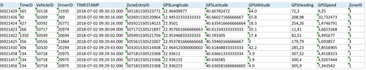
The taxi association that owns the raw data has a long-term collaboration with the Center of Research and Technology Hellas - Hellenic Institute of Transport (CERTH-HIT), which has agreed to provide the dataset for research purposes. The data is pseudo-anon-ymized by CERTH-HIT in order to respect the privacy of the drivers, complying with GDPR article 32 regarding “Security of Processing”, and no connections can be inferred from the raw data to a specific driver and his behavior. This is not a limitation to our study, as we will only use the FCD to extract speeds and traffic conditions of the road network of Thessaloniki, without investigating drivers’ habits and characteristics. Our dataset was extracted from two different tables of a Relational Database Management Systems (RDBMS). The raw data format and feature columns between those tables were not identical, which necessitated the development of two data preprocessing modules to transform data in the same format and unify the in the same data table.
In detail, the raw data is in structured, tabular form and composed of vehicle location (GPS longitude and latitude coordinates), timestamp, orientation, vehicle ID and speed as illustrated in [Figure 4], which consists of some data records from a time period prior to the one that was utilized for this study. A binary variable about the taxi status (empty
or with a passenger) is also provided. Each vehicle’s signals are transmitted and recorded in a CERTH’s database every 10 to 12 seconds or when the vehicle travels a distance of about 100m. For this study, a subset of this database was used, with data for a duration of 3 typical weekdays, from Monday 17th September to Wednesday 19th September 2018. Vehicle IDs are pseudo-anonymized in order for our study to comply with current GDPR regulations, and to respect drivers’ privacy. During each day, the number of operating taxis varies from 800 to 1000 vehicles
Figure 4: Sample data from taxi GPS signals. Timestamps do not correspond to the dataset used for further analysis.
4.1.2 The digitized road network of Thessaloniki
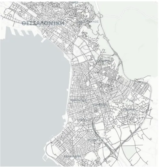
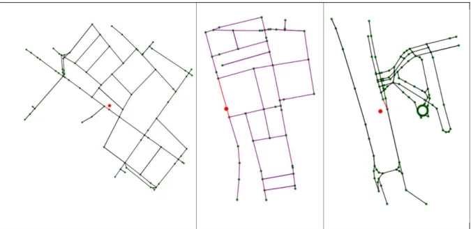
The digitized road network for the region of Thessaloniki was downloaded from the Open Street Maps (OSM) project [46]. This project creates accurate geographical data and maps, for all the world and distributes them free. The data was downloaded to Python using the OSMnx library, developed by Geoff Boeing [47]. This package enables devel-opers to download boundary shapes and street networks from anyplace, using just a cou-ple of lines in their code. The downloaded street networks are based on OSM data and are NetworkX graph objects. NetworkX is Python’s most developed library for efficient manipulation of complex graphs [48] and incorporates numerous functionalities for graph analysis. For our study, the road network of Thessaloniki was downloaded in its detailed form [Figure 5], and it consists of 18055 nodes and 30672 edges. The developer has ac-cess to further details about the network and its topology. Each node has a unique OSMid and is characterized as a point geometric object, with the exact corresponding coordinates. Each edge is a line-string geometric object connecting to points, corresponding to an
ex-ID TimeID VehicleID DriverID TIMESTAMP ZoneEntryID GPSLongitude GPSLatitude GPSAltitude GPSHeading GPSSpeed ZoneID 26921429 165 50118 21935 2018-07-02 09:30:33.000 501181530523771 22.96409977 40.60782472 64.0 72,3 9,25 3 26921426 90 50269 269 2018-07-02 09:30:16.000 502691530520964 22.94532333333333 40.66027166666667 65.8 208,98 10,732473 3 26921424 427 50592 20771 2018-07-02 09:30:16.000 505921530514523 22.9501 40.635416666666664 18.3 254,26 1,4746791 3 26921423 266 50717 20974 2018-07-02 09:30:04.000 507171530521897 22.957661666666663 40.61334333333333 20.1 11,41 3,6653368 3 26921422 1350 50549 20694 2018-07-02 09:30:02.000 505491530521706 22.95346833333333 40.593305 17.4 82,51 6,491677 3 26921425 356 50556 21864 2018-07-02 09:29:44.000 505561530521007 22.953781666666668 40.59460166666667 0 179,79 5,693857 3 26921430 306 50320 20294 2018-07-02 09:29:43.000 503201530514408 22.964525000000002 40.61848833333333 42.2 285,23 7,8556905 3 26921458 234 50718 20975 2018-07-02 09:29:34.000 507181530523368 22.93611 40.63661333333334 3.9 307,52 4,4518323 1 26921457 234 50718 20975 2018-07-02 09:29:33.000 507181530523368 22.936155 40.636585 3.9 300,4 4,9207444 1 26921456 234 50718 20975 2018-07-02 09:29:32.000 507181530523368 22.936215 40.636581666666665 4.0 305,9 7,343542 1
speed limit, length, width, one-way or not. However, for most streets many of those fields are blank, meaning that no data is available.
Figure 5: The full network of the region of Thessaloniki (left) and zoomed in view over the White Tower area(right).
4.2 Data Preprocessing
During preprocessing, data are imported in PySpark, in a tabular format utilizing one of its most efficient and widely used API for data processing, the SQL API. Datatype checks and conversions ensure that data will be in appropriate format for the later stages of anal-ysis. Furthermore, the dataframe is filtered to include GPS signals within the area of in-terest, defined as the bounding box with longitude and latitude values in the ranges [22.91,23.001] and [40.575,40.65] respectively, following the Coordinate Reference Sys-tem (CRS) WG84. This bounding box includes the area of Thessaloniki shown in [Figure 6].
Figure 6: The area inside the defined bounding box and the street network on it.
More filters are applied to the data, in order to ensure quality of records. GPS data are known to include recording errors, for instance highly inaccurate instantaneous speeds, and in bibliography it is considered appropriate to ignore such signals [49]. Therefore, records with speeds exceeding 120km/h are also filtered out, following the methodology proposed in [50]. At the end of the preprocessing step, the Spark dataframe consists of 132.227 records and the five columns meaningful for this project [Table 2].
Table 2: A sample of 10 records from the preprocessed dataframe.
4.3 The Concept of Map-Matching
In recent research studies, scientists follow two different approaches when analyzing GPS data. Some focus on coarse-grained results and divide the research area in a grid of equal in size cells, thus making it straightforward and computationally inexpensive to match each signal to its corresponding cell. Other studies require results in higher detail, which means that GPS records have to be matched to the correct link of the digitized network, a process called map-matching. This is a crucial step that must produce accurate match-ings for subsequent analysis. It includes complicated challenges, considering that it is normal for GPS coordinates to deviate from the exact location of a vehicle [Figure 7]. The factors resulting in such deviations are two [51], the sensor quality and the environ-ment. Higher quality sensors tend to produce more accurate coordinate records, while obstacles and tall structures, like multistory buildings and tunnels in urban environments, highly affect any device’s signal.
Figure 7: Recorded GPS traces of a taxi travelling at Tsimiski Street, captured at a frequency of 1Hz
Several map-matching algorithms have been proposed and tested in recent years, both from academia and industry. Examples include Bayesian probabilistic approaches, Hid-den Markov Models, local characteristics and statistics of road networks, weighted net-works etc. Some algorithms are preferred for sparse datasets with low frequency records and considerable distance between points, while others are optimized to handle denser GPS datasets. Some of the aforementioned algorithms have to be applied on a sequence of datapoints generated by the same vehicle, as the map matching result is affected by the position of the vehicle in previous time steps. Unfortunately, the FCD utilized for this study are pseudo-anonymized, which prohibits the extraction of unique vehicle trajecto-ries on the street network.
A developer can alternatively use map-matching services taking advantage of cloud technologies and implementations from Google, Microsoft and project OSRM (Open Street Routing Machine). Google’s “Snap to roads” service from “Roads API” and Mi-crosoft’s “Snap to Road API” were tested and perform very fast and with exceptional accuracy, however these on-demand cloud services are not free. To the best of the authors knowledge, project OSRM is the only free map-matching provider. Unfortunately, the API almost always returns 429 errors ("Too Many Requests") as it is oriented for demo use only.
Since the aforementioned ready to use algorithms could not be applied, a map-match-ing algorithm was developed from scratch, especially for this study, mappmap-match-ing each data-point to the closest network link. This algorithm’s performance is considered adequate for this study, considering that GPS accuracy in our specific dataset is high [Figure 7] and deviations from real position are in the order of some meters at most.
4.3.1 Point to link distance
This section explains the methodology for calculating distance between any point and road link, a function utilized by our map-matching algorithm. The calculations are
exe-Shapely [52], a well-known Python module for creating and working with planar geomet-ric objects.
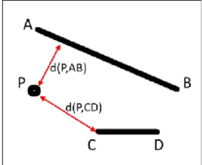
Let d(P,l) denote point’s P distance to a road link l. To calculate d(P,l), the algorithm checks if the point projects onto the line segment. If it does, then d(P,l) is the orthogonal distance from the point to the line is calculated. Otherwise, the distance of P to both link endpoints is calculated and d(P,l) is the shortest one [Figure 8].
Figure 8: The distance of point P from two road links AB and CD. P projects onto AB, but not onto CD.
4.3.2 Map-matching algorithm
Since the road network of Thessaloniki includes more than 30.000 edges, it is prohibited to perform distance calculations and comparisons of every GPS pulse to all edges. Two different approaches were developed and tested. The first one receives a point P to map-match, and then calculates a subgraph G` of the whole network, which is centered at P using a radius of 200m. All distances of P to any edge of G` are calculated, and P is matched to the edge with the lowest distance. This approach proved to be unacceptably slow for the purpose of our study, considering a huge number of points. Distance calcu-lations and comparisons where completed in acceptable time, however extracting a sub-graph for each point is computationally too expensive. As a result, an improved, more efficient algorithm was developed with the objective of utilizing less subgraphs. To achieve this, datapoints are initially clustered into a predefined number of groups and then points of the same group are matched using one subgraph for the whole cluster. In detail, clustering is completed considering a 30x30 grid over the area of interest. Each datapoint is assigned to one of the 900 grid cells and then all points of each cell are map-matched
calculating the distances from the subgraph G` that covers the geographic area of the corresponding cell. The improved algorithm proved to be immensely more efficient than the initial, due to the fact that the number of subgraphs used is equal to the number of grid cells, and therefore constant, independently of the number of points to be matched.
Figure 9: Three GPS points (red) and the corresponding network edge they are matched to (red).
The final map-matching step is considering speed orientation of the GPS signals. The Open Street Maps network downloaded has classified all road links as one-way or two-way. For each two-way road, the two opposite directions are calculated as degrees of anti-clockwise deviation from North, the same orientation system used in the GPS dataset. Then, all datapoints corresponding to two-way roads are matched to the appropriate di-rection comparing GPS signal and road orientation.
Figure 10: Pseudo-code of the complete map-matching algorithm.
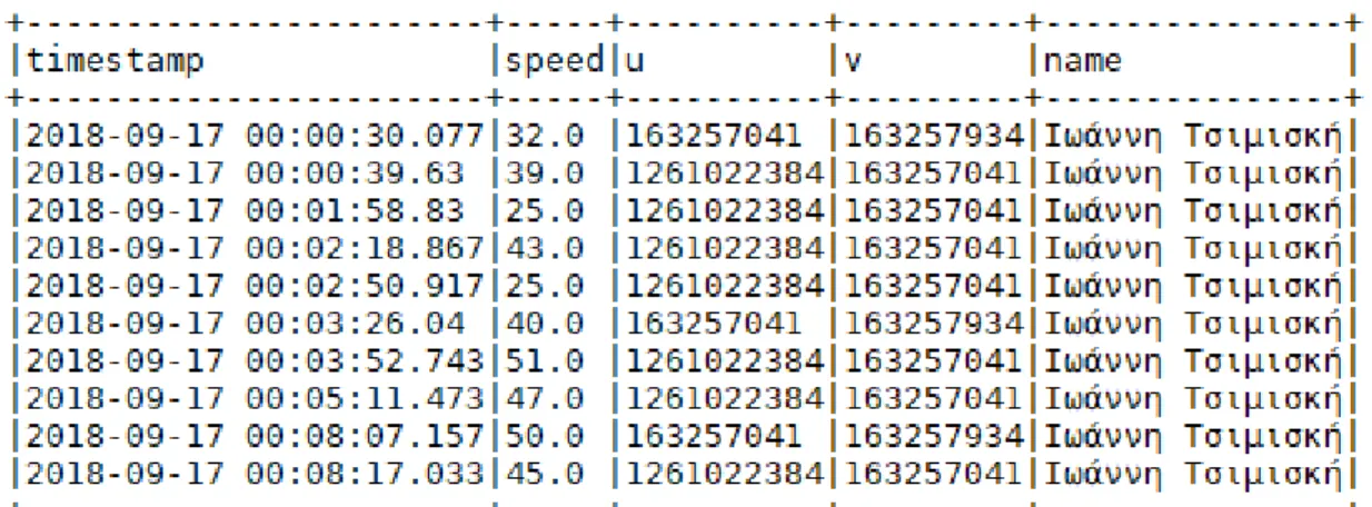
After the map-matching procedure, the dataframe consists of five columns, timestamp, speed, the node ID of the start and the end of the link respectively and the street name, as shown in Table 3. For example, the first record of Table 3 is matched to the road link that starts at node with ID 163257041 and ends at node with ID 1632257934.
Table 3: A sample of 10 records of the map-matched dataset.
4.4 Time series transformation
After all data points have been matched to the corresponding roads, further processing steps take place in order transform data in time series, grouping together the records for the same road and time interval. In our model, we consider 15-minute intervals, on the
basis that the prediction model should forecast traffic congestion for the near future. As already stated in the literature review section, models for longer time intervals have been successfully implemented but this is not the scope of this research project. Moreover, this implementation utilizes state-of-the-art distributed computation technology to take ad-vantage of the computational capabilities, fast processing and results production irrespec-tive of dataset size.
4.5 Data limitations and formulation of the
predic-tive algorithm
At this point the researcher was faced with a limitation derived from the amount of available data and its consistency. It was expected that available data would not cover all Thessaloniki network consistently for every 15-minute time interval. However, after map-matching and time grouping it was apparent that only a small number of roads in the center of the city (mainly Tsimiski str.) had consistent speed records. After discussions with experts from the Hellenic Institute of Transport, which collaborate closely with the taxi association for years, the significant lack of data is the result of the following factors: 1. After the economic crisis in Greece, the majority of taxi drivers choose to wait in taxi stops rather than circulating when searching for customers, in order to mini-mize operational costs.
2. Customers nowadays prefer to call for taxis using internet services, rather than waiting for a random taxi, another factor that has affected circulation.
3. Increased fuel cost.
Data on Tsimiski street are adequately dense because it is a three-lane road crossing the heart of Thessaloniki city center and is usually busy 24 hours a day. Furthermore, the frequency of GPS pulses from some taxis is increased to 1Hz at this area, as a result of a completed scientific project. For the following steps towards the implementation of the traffic forecasting algorithm, only the subset of pulses map-matched on Tsimiski street were used.
data-consistent road links of approximately the same length. The final three road sections that were created cover all the length of Tsimiski street. The task of the machine learning algorithm was defined as follows: build a forecasting tool for the average speed of the middle section (section 2) at any time interval t, utilizing historical data for all three sec-tions. The term historical refers to any data collected before interval t.
4.6 Feature Extraction
Having grouped the data points is both dimensions of time (time interval) and space (road section), more statistics were extracted from the distributions of speed. For each time interval and road section, the derived statistics are:
• average speed,
• standard deviation of speed,
• count of pulses, • maximum speed, • distribution skewness, • 60% percentile, • 80% percentile as shown in [Table 4].
Table 4: Processed dataset for one road section
Furthermore, the time interval was encoded in a cyclical fashion, considering one day as a circle. A circle (24h) consists of N=96 15-minute intervals, therefore each interval i=0, 1, 2, ... ,96 is mapped to its corresponding angle of θ =(2pi*n)/96 rad and is coded to the tuple (sinθ,cosθ). Consecutive time intervals are mapped to angles with a minimum difference of (2pi)/96 rad, and thus coded to tuples with small sine and cosine difference.
Distant intervals are coded to tuples which are significantly different, for example two intervals with 12-hour time difference are 48-time intervals away and are therefore coded to angles with a difference of (2pi)48/96= pi rad, producing angle codings with opposite sings. This tuple was used to train models when the train set was not perceived as a timeseries with specific steps, in order to incorporate the cyclical (seasonal) effect of time in traffic conditions.
5
Results
In this section the results from the different predictive algorithms implemented for traffic forecasting are discussed.
5.1 Machine Learning Algorithms
PySpark offers a machine learning library (ML) with numerous utilities and functions [53] which enable the construction of a variety of machine learning models for all differ-ent kinds of problems, including classification, regression, clustering. The objective of our proposed technique is speed prediction, which in principal is a regression problem. It is also possible to formulate speed prediction as a classification problem, inferring differ-ent classes according to the deviation of predicted speed from the speed limit of the tar-geted road section. Our approach follows the regression methodology, which provides fine-grained results of higher resolution, while also enabling the researcher to monitor the model’s performance closely, with numerous evaluation techniques. For the purpose of this study, three of the most well-known machine learning algorithms for regression avail-able in PySpark were utilized. Namely, these algorithms are Multiple Linear Regression, Random Forest and Gradient Boosting. In the following paragraphs follows a short sum-mary of the principles on which each of the aforementioned algorithms is based on. The formal mathematical foundations and definitions of those algorithms is out of the scope of this study.
5.1.1 Multiple Linear Regression
A multiple linear regression algorithm attempts to model the relationship between two or more explanatory variables and a response variable by fitting a linear equation to observed data. It assumes that every value of the independent variable x is associated with a value
of the dependent variable y. Formally, the model for multiple linear regression, given n observations, is
𝑦𝑖 = 𝑎0 + 𝑎1𝑥𝑖,1 + 𝑎2𝑥𝑖,2 + . . . 𝑎𝑛𝑥𝑖,𝑛 + 𝑖 𝑓𝑜𝑟 𝑖 = 1,2, . . . 𝑛.
5.1.2 Random Forest Regression
Random forests are regression algorithms which combine a – usually big- number of tree predictors in such a way that a tree depends on the values of a random vector sampled independently and with the same distribution for all trees in the forest. Such predictive algorithms, based on numerous individual predictors, belong to the category of ensemble methods.
5.1.3 Gradient Boosting Trees Regression
Gradient boosting regression also belongs to the family of ensemble methods. Typically, it utilizes a user specified number of decision trees as individual predictors. During the learning process, the loss function is minimized by adding weak learners using the gradi-ent descgradi-ent technique.
5.2 Evaluation Techniques and Metrics
The developed machine learning models were evaluated through the process of 10-fold cross-validation. This procedure randomly splits the train set to ten mutually exclusive subsets, and recursively trains the model on nine of them, using the tenth subset for eval-uation. Once the 10 folds are completed, the algorithm reports the evaluation metric for each fold and the researcher can evaluate the model in a more generic fashion, examining its capabilities on different training and test sets.
The regression evaluation metrics that were monitored in this study include the mean of squared errors of predictions, root of mean squared errors, and the mean of absolute
5.2.1 Mean of squared errors
The mean of squared errors (mse) evaluation technique is the average squared difference between the actual and predicted values of a variable. As a result, it is always non-nega-tive, with smaller values indicating better predictive performance. It is important to re-member that it is expressed as squared units of the estimated quantity, and due to its mathematical formulation, it weighs large errors more heavily.
5.2.2 Root mean of square errors
The root of the mean of squared errors (rmse), also called as root of mean square devia-tion, is calculated as the square root of mse. Unlike the mse, it is expressed in the same units as the estimated quantity, however the rmse is also non-negative and also sensitive to outliers as larger errors have a disproportionately large effect on it.
5.2.3 Mean of absolute errors
The mean absolute error (mae) is calculated as the mean of the absolute values of errors. Compared to the rmse and mse, it is the easiest to interpret due to the simplicity of its mathematical formula. Mae is also non-negative and just like the mse and rmse it sum-marizes estimation accuracy without distinguishing over-predictions from under-predic-tions. Large and low estimation errors have proportional effect on the mae.
5.3 Model tuning
The algorithms utilized for traffic speed estimation were all fine-tuned in an attempt to improve estimation accuracy. Model tuning was implemented based on the grid-search cross-validation technique, according to which the developer selects a set of parameters with user defined values (called hyperparameters) to be tested. Respective values for each hyperparameter are also specified, and an exhaustive grid of all parameter value combi-nations is created. The model is trained on every combination of parameters, in order to detect the optimal hyperparameter values.
5.4 Forecasting results
In order to compare amongst the performance of different regression models, all models were developed considering the same loss function to minimize, in this case the mean squared error. The choice was made because of the evaluator’s characteristics. Mse is expressed in km per hour, a value easier to interpret than the rmse. However, it is not to be confused with the even simpler expression of mae. The mse was favored against the mae, for penalize more the large estimation errors. The proposed model predicts the av-erage speed of a road and therefore predictions with small positive or negative error should not be weighted proportionally to larger errors. In plain words, the model is not so strict against small estimation errors, but it penalizes large errors disproportionally more.
In principle, there is no proven theory on which hyperparameter values would work better at each problem, and as a result tuning is achieved through grid search cross vali-dation, a try-and-error procedure during which the optimum combination of hyperparam-eter values is detected. The random forest and gradient boosting trees regressors both have a number of different hyperparameters to be tuned, and exhaustive grid search with 10-fold cross-validation was applied on most hyperparameters as Table 5 shows.
Table 5: Grid-search cross-validation for random forest and gradient boosting algorithms.
Regression algorithm Hyperparameter Grid search values
Random Forest
Maximum tree depth [3, 5, 7]
Subsampling rate [0.8 , 1, 1.2 ]
Impurity criterion Only supported option is variance
Number of trees [ 50, 100, 200, 300]
Gradient Boosting Trees
Maximum tree depth [3, 5, 7]
Subsampling rate [0.8 , 1, 1.2 ]
Impurity criterion Only supported option is variance
Number of trees [ 50, 100, 200, 300]
The random forest regressor performed better on the combination of 100 trees of max-imum depth of five and subsampling rate 1, while gradient boosting best configuration was 50 trees of depth five and also with subsampling rate equal to 1. In general, random forest performed significantly better than gradient boosting and slightly better than the linear regression model. All evaluation metrics of the three models, with optimized hy-perparameters, are summarized in Table 6.
Table 6: Evaluation Metrics of tested algorithms
Regression algorithm mse rmse mae
Random Forest 4.74 22.48 3.10
Linear regression 4.79 22.98 3.73
6
Conclusion
During the last years Intelligent Transportation Systems (ITS) that utilize data processing algorithms are developed in unprecedent rate. Such innovative systems provide Trans-portation planners and decision makers with critical tools and knowledge for improving the general efficiency of the existing infrastructure. Positive results are profound in mul-tiple sectors, amongst which are economy, road safety and monitoring. As the volume of transportation data increases, certain systems and algorithms will inevitably need to be implemented in technologies able to handle the so-called ‘Big Data’, huge volumes of data arriving at huge speed from different sources. This project’s primary goal was to inspect the suitability of PySpark, Python’s API for distributed programming language Spark, for developing a traffic forecasting model.
The most important findings and lessons learned from this research study are summa-rized below:
• PySpark is indeed a very powerful technology that provides a plethora of ready to use functionalities and libraries for data processing tasks. Raw data can be arbi-trarily big, as PySpark is designed to run on parallel utilizing a cluster of ma-chines. A characteristic that proved very helpful to the author is that PySpark code can be developed and run using a Python Integrated Development Environment (Python IDE) like Spyder. Taking into consideration that PySpark’s programing interface has profound similarities with Python, the transition of algorithms de-veloped to run locally with Python, to PySpark is to a very great extent seamless.
• PySpark does pose certain limitations regarding the variety of available built-in machine learning algorithms, when compared to the algorithms available on the most widely-used platforms like Python. However, as also stated in paragraph 3.3.3, it is a relatively new programming language that has been around for four and a half years, currently supported and developed by Apache. The author’s opin-ion is that available functopin-ionalities will keep increasing in the near future.
• The developed tool is proof that a real time traffic monitoring application with high predictive performance can be implemented on a large scale utilizing big data technologies.
• In order to achieve a real-world traffic forecasting tool for the whole scale of a city’s network, the level of penetration of GPS-equipped vehicles should be con-siderably high, to ensure constant network-wide data generation. This is a serious limitation the developer needs to take into consideration. However, with Internet of Things (IoT) enabled devices and increasing data availability the author be-lieves that in the near future this hurdle will be overcome.
7
Future Prospects
In this section the author states his opinion on actions that could take place in the future in order to improve the proposed traffic forecasting system. The traffic forecasting tool implemented for this master’s dissertation project certainly reveals that big data technol-ogies can successfully be adopted by the Transportation sector. However, certain stages and modules of the system can be significantly improved in the future.
The author suggests that the most important improvement could result from a dataset of larger volume, as the dataset utilized for this study is limited both in terms of time duration and vehicle penetration. Machine learning algorithms are well known for their ability to ‘learn’ patterns from huge datasets with millions of records and it is expected that a model trained on several months of data could perform more accurately on predict-ing speeds. Such a model could also be trained on some more extreme scenarios, like days with extreme weather conditions or days when vehicle circulation is affected by closed roads due to riots or other events. In addition, higher vehicle penetration would lead to data availability for more streets, enabling the development of larger scale models with more input variables.
Furthermore, the author believes that there is room for improvement in the map-matching section. The custom map-map-matching algorithm that was developed for this study, although computationally efficient, is distance-based and does not consider the sequence of unique vehicle signals, like some more advanced algorithms provided by Google and Microsoft.
8
Bibliography
[1] D. Laney, «3D Data Management: Controlling Data Volume, Velocity, and Variety,» Application Delivery Strategies, 2001.
[2] V. Usyukov, "Methodology for identifying activities from GPS data streams," in
The 8th International Conference on Ambient Systems, Networks and Technologies, 2017.
[3] M. Houbraken, S. Logghe, P. Audenaert, D. Colle and M. Pickavet, "Examining the potential of Floating Car Data for Dynamic Traffic Management," IET Intelligent Transport Systems, 2018.
[4] K. Adam and V. Athena, "Real-time Traffic Prediction using Multiple Data Sources," Department of Informatics, Aristotle University of Thessaloniki, Thessaloniki, 2018.
[5] J. Barros, M. Araujo and R. J. Rossetti, "Short-term real-time traffic prediction methods: a survey," in Models and Technologies for Intelligent Transportation Systems (MT-ITS), Budapest, Hungary, 2015.
[6] K. Diependaele, F. Riguelle and P. Temmerman, "Speed behavior indicators based on floating car data: results of a pilot study in Belgium," Transportation Research Procedia, p. 2074 – 2082, 2016.
[7] L. Mannini, E. Cipriani, U. Crisalli, A. Gemma και G. Vaccaro, «On-Street Parking Search Time Estimation Using FCD Data,» Transportation Research Procedia, p. 929–936, 2017.
[8] S. Suhas, V. Kalyan, M. Katti, A. Prakash and C. Naveena, "A Comprehensive Review on Traffic Prediction for Intelligent Transport System," in International Conference on Recent Advances in Electronics and Communication Technology, 2017.
[9] C. d. Fabritiis, R. Ragona and G. Valenti, "Traffic Estimation And Prediction Based On Real Time Floating Car Data," in Proceedings of the 11th International IEEE Conference on Intelligent Transportation Systems, Beijing, China, 2008.
[10] J. Rzeszótko and S. H. Nguyen, "Machine Learning for Traffic Prediction,"
Fundamenta Informaticae, pp. 407-420, 2012.
[11] H. Yi, H. Jung and S. Bae, "Deep Neural Networks for Traffic Flow Prediction," in
IEEE International Conference on Big Data and Smart Computing (BigComp), Jeju, South Korea, 2017.
[12] T.-I. Theodorou, A. Salamanis, D. D. Kehagias, D. Tzovaras and C. Tjortjis, "Short-Term Traffic Prediction under Both Typical and Atypical Traffic Conditions using a Pattern Transitions Model," in Proceedings of the 3rd International Conference on Vehicle Technology and Intelligent Transport Systems (VEHITS 2017), 2017.
[13] A. Sunderrajan, V. Viswanathan, W. Cai and A. Knoll, "Traffic State Estimation Using Floating Car Data," in The International Conference on Computational Science, 2016.
[14] M. Thottan and C. Ji, "Anomaly Detection in IP Networks," IEEE Transactions on Signal Processing, vol. 51, no. 8, 2003.
[15] X. Liu, X. Liu, Y. Wang, J. Pu and X. Zhang, "Detecting Anomaly in Traffic Flow from Road Similarity Analysis," in 17th International Conference, WAIM 2016 International Conference on Web-Age Information Management, Nanchang, China, 2016.
[16] W. Kuang, S. An and H. Jiang, "Detecting Traffic Anomalies in Urban Areas Using Taxi GPS Data," Mathematical Problems in Engineering, vol. 2015, 2015.
[17] B. Pan, Y. Zheng, D. Wilkie and C. Shahabi, "Crowd sensing of traffic anomalies based on human mobility and social media," in SIGSPATIAL'13 Proceedings of the 21st ACM SIGSPATIAL International Conference on Advances in Geographic Information Systems, Orlando, Florida, 2013.
[18] W. Liu, Y. Zheng, S. Chawla, J. Yuan and X. Xie, "Discovering Spatio-Temporal Causal Interactions in Traffic Data Streams," in KDD '11 Proceedings of the 17th
ACM SIGKDD international conference on Knowledge discovery and data mining, San Diego, California, USA, 2011.
[19] J. Zhang, "Smarter outlier detection and deeper understanding of large-scale taxi trip records: a case study of NYC," in Proceedings of the ACM SIGKDD International Workshop on Urban Computing, Beijing, China, 2012.
[20] D. Zhang, N. Li, Z.-H. Zhou, C. Chen, L. Sun and S. Li, "UbiComp '11 Proceedings of the 13th international conference on Ubiquitous computing," Beijing, China, 2011.
[21] C. Chen, D. Zhang, P. S. Castro, N. Li, L. Sun and S. Li, "Real-Time Detection of Anomalous Taxi Trajectories from GPS Traces," in International Conference on Mobile and Ubiquitous Systems: Computing, Networking, and Services, Copenhagen, Denmark, 2011.
[22] Y. Ge, H. Xiong, C. Liu and Z.-H. Zhou, "A Taxi Driving Fraud Detection System," in ICDM '11 Proceedings of the 2011 IEEE 11th International Conference on Data Mining, Washington, DC, USA, 2011.
[23] Y. Ge, C. Liu, H. Xiong and J. Chen, "A taxi business intelligence system," in KDD '11 Proceedings of the 17th ACM SIGKDD international conference on Knowledge discovery and data mining, San Diego, California, USA, 2011.
[24] P. S. Castro, D. Zhang, C. Chen, S. Li and G. Pan, "From Taxi GPS Traces to Social and Community Dynamics: A Survey," ACM Comput. Surv. 46, 2, Article 17, 2013.
[25] L. Liu, C. Andris and C. Ratti, "Uncovering cabdrivers’ behavior patterns from their digital traces.," Comput. Environ. Urban Syst., vol. 34, no. 6, p. 541–548., 2010.
[26] J. Yuan, Y. Zheng, X. Xie and G. Sun, "Driving with knowledge from the physical world," in Proceedings of the ACM SIGKDD International Conference on Knowledge Discovery and Data Mining, 2011.
[27] J. Yuan, Y. Zheng, X. Xie and G. Sun, "Where to find my next passenger?," in
Proceedings of the International Conference on Ubiquitous Computing, 2011.
[28] V. Astarita, V. P. Giofrè, G. Guido and A. Vitale, "The Use of Adaptive Traffic Signal Systems Based on Floating Car Data," Wireless Communications and Mobile Computing, vol. 2017, 2017.
[29] G. A. Klunder, H. Taale, L. Keste and S. Hoogendoorn, "Improvement of Network Performance by In-Vehicle Routing Using Floating Car Data," Journal of Advanced Transportation, vol. 2017, 2017.
[30] M. Jahnke, L. Ding, K. Karja and S. Wang, "Identifying origin/destination hotspots in floating car data for visual analysis of traveling behavior," in 13th Location-Based Services Conference, LBS 2016, Vienna, Austria, 2016.
[31] M. Cocca, D. Giordano, M. Mellia and L. Vassio, "Free Floating Electric Car Sharing in Smart Cities: Data Driven System Dimensionung," in IEEE International Conference on Smart Computing, 2018.
[32] J. Zhang, G. Song, D. Gong, Y. Gao, L. Yu and J. Guo, "Analysis of rainfall effects on road travel speed in Beijing, China," IET Intelligent Transport Systems, vol. 12, pp. 93-102, 2018.
[33] Z. Shaojun, N. Tianlin, W. Ye, Z. Max and T. J. Wallington, "Fine-grained vehicle emission management using intelligent transportation system data," in
Environmental Pollution, 2018, pp. 1027-1037.
[34] C. Liberto, G. Valenti, S. Orchi, M. Lelli, M. Nigro and M. Ferrara, "IEEE Transactions on Intelligent Transportation Systems," 2018.
[35] Y. Du, J. Wu, S. Yang and L. Zhou, "Predicting vehicle fuel consumption patterns using floating vehicle data," Journal of Environmental Sciences, vol. 59, pp. 24-29, 2017.
[36] J. M. S. Grau, I. Toumpalidis and E. Chaniotakis, "Correlation between digital and physical world, case study in Thessaloniki," 2018.
[37] L. Montini and N. Rieser-Schüssler, "Trip Purpose Identification from GPS Tracks," Transportation Research Record Journal of the Transportation Research Board, 2014.
[38] Q. Guande, L. Xiaolong and L. Shijian, "M