Safety Based Decision Support Systems For Marine Structures

(1)

ISTANBUL TECHNICAL UNIVERSITY

 INSTITUTE OF SCIENCE

SAFETY BASED DECISION SUPPORT SYSTEMS FOR MARINE

STRUCTURES

M.Sc. THESIS,

Emre Koray GENÇSOY,

Department of Naval Architecture and Marine Engineering,

Naval Architecture and Marine Engineering Programme,

(2)

(3)

ISTANBUL TECHNICAL UNIVERSITY

 INSTITUTE OF SCIENCE

SAFETY BASED DECISION SUPPORT SYSTEMS FOR MARINE

STRUCTURES

M.Sc. THESIS,

Emre Koray GENÇSOY,

508981001

Department of Naval Architecture and Marine Engineering,

Naval Architecture and Marine Engineering Programme,

Thesis Advisor : Assoc. Prof. Dr. ġebnem Helvacıoğlu

(4)

(5)

Emre Koray GENÇSOY, a M.Sc. student of ITU Institute of Science, student ID 508981001, successfully defended the thesis entitled “

SAFETY BASED

DECISION SUPPORT SYSTEMS FOR MARINE STRUCTURES

”, which he prepared after fulfilling the requirements specified in the associated legislations, before the jury whose signatures are below.

Thesis Advisor : Assoc. Prof. Dr. ġebnem HELVACIOĞLU

Istanbul Technical University

Jury Members : Ass. Prof. Dr. Yalçın ÜNSAN

Istanbul Technical University

Ass. Prof. Dr. Serhan GÖKÇAY

Piri Reis University

DATE OF SUBMISSION: 11 AUGUST 2016 DATE OF DEFENCE: 15 AUGUST 2016

(6)

(7)

Dedicated to

(8)

(9)

FOREWORD

My post graduate journey started on 1998, after two years of study; I was ready to start working on my thesis. Several attempts to choose a subject to study has fallen down by me. I desired to work on new applications for marine industry which may be a new step for further studies. After 16 years of working on different subjects, finally here I am.

First of all, I would like to thank to my beloved mother, she was my shining pole star that lightens my course. She is the reason of who I am.

Prof. Dr. A. Yücel Odabaşı is an important figure of my entire engineering career, I have learned a lot from him and used what I have learnt in every single engineering problem I face. I always feel myself lucky and proud of being his student.

These two important figures of my life are both passed away during all those years. I will always be grateful to them for enriching my life.

Assoc. Prof. Dr. Şebnem Helvacıoğlu; if she was not so encouraging, for sure, I will not able to be at this point. I do thank a lot for all of her patience, excellent guidance, advice and her support.

And my dear family;

My sister PhD. Elif Banu Gençsoy, thanks for all of her efforts that helped me to deal with procedures and regulations of the university.

My wife Özlem, for standing next to me during all those years of study with her patience.

And of course, my little son Kuzey, thank you for adding priceless values to my life, this is for you.

(10)

(11)

1 INTRODUCTION ... 1

1.1 Scope and Limitations ... 2

2 LITERATURE REVIEW ... 5 2.1 Risk Management ... 5 2.2 Risk Assessment ... 7 2.2.1 Risk identification ... 8 2.2.2 Risk analysis ... 9 2.2.3 Risk evaluation ... 9 2.3 Risk Treatment ...10

2.4 Multiple Criteria Decision Making Methods ...10

2.4.1 Pairwise comparison ...13

2.4.2 Solving matrices ...14

2.4.3 Dealing with inconsistency ...15

2.4.4 Rank reversal ...16

2.4.5 Group decision making ...16

2.4.6 AHP versus ANP ...19

2.4.7 Fuzzy-ANP and ANP comparison ...21

2.4.8 Fuzzy-ANP methodology ...22

2.4.9 Chang’s extent analysis methodology ...22

2.4.10 Scales used in comparisons ...24

3 CASE STUDY ... 25

3.1 Safety and Environmental Issues of LNG ...25

3.2 Bunkering Operation (Truck to Ship) ...26

3.3 Risks of Bunkering Operation ...26

3.3.1 Fault tree analysis (FTA) ...27

3.3.2 Analytical network process (ANP) structure ...32

3.3.3 Questionnaire ...34

3.3.4 Ranking of decision makers ...39

3.3.5 Calculating group decision ...40

3.3.6 Calculation of risk value for alternatives ...43

4 CONCLUSION ... 45

REFERENCES ... 47

APPENDICES A: BUNKERING ... 51

A.1 Bunkering Operation Diagram ...51

APPENDICES B: HAZARD DEFINITIONS ... 55

APPENDICES C: CLUSTERS INNER AND OUTER RELATIONS ... 57

APPENDICES D: QUESTIONNAIRE AND EXPERT REPLIES ... 63

D.1 Questionnaire for clusters - Consequences ...63

(12)

D.3 Questionnaire for nodes - Consequences ... 65

D.4 Questionnaire for nodes - Likelihood ... 75

APPENDICES E CALCULATION SHEETS FOR ANP ... 85

APPENDICES F CALCULATION SHEETS FOR FUZZY-ANP ... 159

APPENDICES G SUPERDECISIONS ANP MODEL ... 233

APPENDICES H EXCEL VBA CODES ... 237

APPENDICES I CALCULATION OF DECISION MAKERS’ RANKS ... 245

(13)

ABBREVATIONS

AHP : Analytical hierarchy process

AIJ : Aggregation of individual judgments AIP : Aggregation of individual priorities ALARP : As low as reasonable practical ANP : Analytic network process

BOCR : Benefits, opportunities, costs, risks CBA : Cost - benefit analysis

CI : Consistency index CO2 : Carbon dioxide CR : Consistency ratio ECA : Emission control area

ELECTRE : Elimination et choix traduisant la réalité ESD : Emergency shutdown device

ETC : Et cetera (and other things) FMEA : Failure mode and effects analysis FTA : Fault tree analysis

HACCP : Hazard analysis and critical control points HAZID : Hazard identification

HAZOP : Hazard and operability study HFO : Heavy fuel oil

IEC : International Electrotechnical Commission

IGF : International code of safety of ships using gases or other low flashpoint fuels

IMO : International maritime organization

ISO : International Organization for Standardization LNG : Liquefied natural gas

LOPA : Layer protection analysis

MADM : Multiple attribute decision making

MARPOL : International convention for the prevention of pollution from ships MCDA : Multiple criteria decision analysis

MDO : Marine diesel oil

MODM : Multiple objective decision making MSC : Maritime safety committee

N2 : Nitrogen (Inert gas)

NG : Natural gas

NOx : Nitrogen oxides

PHA : Primary hazard analysis

(14)

Sox : Sulphur oxides

SWIFT : Structured what-if technique

TOPSIS : Technique for order of preference by similarity to ideal solution

(15)

LIST OF TABLES

PAGE

Table 2.1: Risk identification methods. ... 9

Table 2.2: List of main AHP/ANP Studies. ...12

Table 2.3: List of Fuzzy Logic and Fuzzy-AHP/ANP Studies. ...13

Table 2.4: Fundamental Scale for Pairwise Comparison. ...14

Table 2.5: Mean Random Consistency Index.(Saaty, 1980) ...16

Table 2.6: Pros and Cons of ANP over AHP ...20

Table 2.7: Scales for pairwise comparison ...24

Table 3.1: Decision Maker 1 Consequences results comparison ...36

Table 3.2: Decision Maker 1 Likelihood results comparison ...37

Table 3.3: Decision Maker 2 Consequences results comparison ...38

Table 3.4: Decision Maker 2 Likelihood results comparison ...39

Table 3.5: Group Decision - Consequences ...41

Table 3.6: Group Decision - Likelihood ...42

Table 3.7: Risk Values...43

Table A.1 : LNG Bunkering Operation ...53

Table C.1: Alternatives Cluster 1 ...57

Table C.2: Alternatives Cluster 2 ...58

Table C.3: Human Cluster ...58

Table C.4: Operations Cluster ...59

Table C.5: Connection Cluster ...60

Table C.6: Environmental Cluster ...61

Table E.1: Unweighted Matrix 1 (Consequences-Decision Maker 2) ...86

Table E.7: Normalized Weighted Matrix 1 (Consequences-Decision Maker 2) ...92

Table E.13: 32th Power of Limit Matrix 1 (Consequences-Decision Maker 2) ...98

Table E.14: 32th Power of Limit Matrix 2 (Consequences-Decision Maker 2) ...99

Table E.15: 32th Power of Limit Matrix 3 (Consequences-Decision Maker 2) ... 100

Table E.19: Unweighted Matrix 1 (Likelihood-Decision Maker 2) ... 104

(16)

Table E.26: Normalized Weighted Matrix 2 (Likelihood-Decision Maker 2)... 111

Table E.31: 32th Power of Limit Matrix 1 (Likelihood-Decision Maker 2) ... 116

Table E.37: Unweighted Matrix 1 (Consequences-Decision Maker 1) ... 122

Table E.43: Normalized Weighted Matrix 1 (Consequences-Decision Maker 1) ... 128

Table F.1: Unweighted Matrix 1 (Consequences-Decision Maker 2) ... 160

(17)

Table F.9: Normalized Weighted Matrix 3 (Consequences-Decision Maker 2) ... 168

Table F.10: Normalized Weighted Matrix 4 (Consequences-Decision Maker 2).... 169

Table F.13: 32th Power of Limit Matrix 1 (Consequences-Decision Maker 2) ... 172

Table F.19: Unweighted Matrix 1 (Likelihood-Decision Maker 2) ... 178

Table F.25: Normalized Weighted Matrix 1 (Likelihood-Decision Maker 2) ... 184

Table F.31: 32th Power of Limit Matrix 1 (Likelihood-Decision Maker 2) ... 190

Table F.37: Unweighted Matrix 1 (Consequence-Decision Maker 1) ... 196

Table F.43: Normalized Weighted Matrix 1 (Consequence-Decision Maker 1) ... 202

Table F.49: 32th Power of Limit Matrix 1 (Consequence-Decision Maker 1) ... 208

(18)

Table I.1: Pairwise comparisons for decision makers’ ranks... 245

Table I.2: Super Matrix ... 246

Table I.3: Limit Matrix ... 246

(19)

LIST OF FIGURES

PAGE

Figure 2.A: Risk Management Steps. ... 6

Figure 2.B: Risk Assessment. ... 8

Figure 2.C: Defining Risk Assessment Items. ... 8

Figure 2.D: AHP Structure ...19

Figure 2.E: ANP Network Structure ...21

Figure 2.F Triangular fuzzy number intersection ...23

Figure 3.A: Emission Reduction Percentage Obtained by gas ...26

Figure 3.B: FTA Symbols ...28

Figure 3.C: Main Hazards ...28

Figure 3.D: NG Leak Hazards ...29

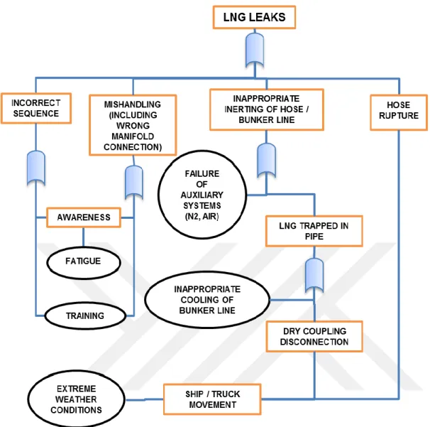
Figure 3.E: LNG Leak Hazards ...30

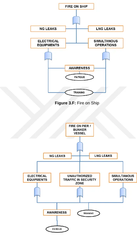
Figure 3.F: Fire on Ship ...31

Figure 3.G: Fire on Pier/Bunker Vessel ...31

Figure 3.H: Control Criteria ...32

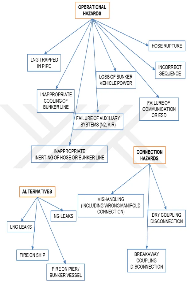
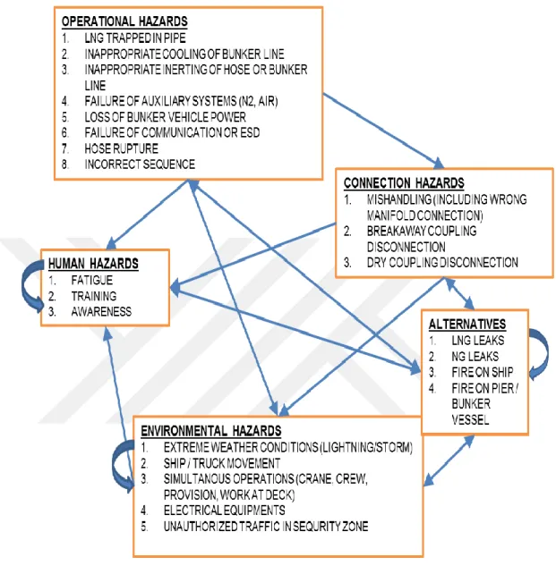
Figure 3.I: Grouped Hazards - 1 ...33

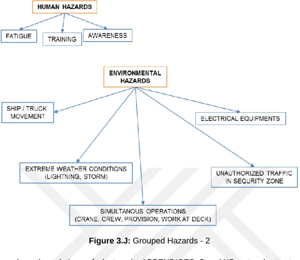
Figure 3.J: Grouped Hazards - 2 ...34

Figure 3.K: ANP Network Structure...35

Figure 3.L: Network structure for decision makers ...40

Figure 3.M: Risk Values ...43

Figure G.A Main model structure ... 233

Figure G.B Consequences sub-model ... 234

Figure G.C Likelihood sub-model ... 234

(20)

(21)

SAFETY BASED DECISION SUPPORT SYSTEMS FOR MARINE STRUCTURES SUMMARY

Analyzing risk is an essential and very powerful tool to deal with uncertainties. New technologies, new developments and new methodologies always include uncertainties and thereby risks. There are many different methods to deal with risks. Qualitative and quantitative methods are both used for decades with success in many different industries. Quantitative studies require more statistical data then qualitative ones. Ability to use both tangible and intangible data in analyses enables to perform risk analysis at any stage of the project. Hazardous Identification (HAZID) and Hazardous and Operability (HAZOP) studies are powerful and widely used analysis methods. In these studies a group of experts make an effort to define and assess possible risks. Work groups may be problematic if group domination by one or more participants happens. And generally because of the consensus about the subject, it is hard to include fuzziness.

Risk assessment is a very important figure in analysis of new systems. Assessment has three main stages; risk identification, risk analysis and risk evaluation. Identification starts with questioning “when, what, who, how, where”, after finding answers to these questions analysis stage starts. Answers to questions at identification stage helps to understand the boundaries of the system. Analysis focuses on “how much, how often, how critical” type questions. These questions help analyst to understand the nature, period and level of risk. After analyzing the risk evaluation period starts; this point is the one where the action to the risk is selected, taking no action or transferring risk such as an insurance company might also be an alternative.

There are several techniques defined by ISO to deal with risk management. About 30 techniques are listed in the standard. Whatever the method is used, knowledge of experts, their understanding of problem and their position to view the risk will directly affect the result. In order to get proper assessment results, problem has to be thought from all sides of aspect. The success is methodology depended, however the main component of all analysis methods is human.

Whether or not be aware of it, decision making is something done in every daily life. Decisions made, draw the path of life, decisions shapes the life and every decision has it’s own consequences that has to be faced. Historically, human decisions theories have focused on outcome prediction. Modern decision making is based on ; understanding of decision making process, thoughts and application of technology tools to support process by human beings. Analytical Hierarchy Process (AHP) proved that using Eigen vectors to solve decision problems is possible. With this study Saaty opened slightly the door to the new studies. Difficulties about modeling real problems in a hierarchical structure are limiting the usage of AHP; therefore a better way of modeling in network structure with dependencies and feedback is presented by Saaty. This methodology is called Analytical Network Process (ANP). ANP is a successful and powerful tool to model complex decision problems. However modeling and solving ANP requires a lot of patience and effort. Fuzzy Multi-Criteria Decision Making using Fuzzy Set Theory has been recommended as an alternative method for overcome the complexity of ANP. Fuzzy sets contain uncertainty and they are easy to apply to all kinds of problems. There are also some

(22)

challenging difficulties with fuzzy sets. Definition of fuzzy sets, membership functions require experience. Changing defined rules is not so easy. Due to these problems in multi-criteria decision making, hybrid methods such as Fuzzy-AHP, Fuzzy-ANP, etc. are being used commonly. There are generated hybrid solution methodologies, thus applier, depending of the nature of the problem, may choose one of them and directly apply the solution method.

In this study, LNG bunkering operation was selected as case study. LNG is one of the most probable alternatives to current fuel oils. Bunkering operation is the most challenging part of LNG usage on board. HAZID/HAZOP studies for bunkering, classification societies bunkering guidelines were used to define the hazards. Hazards are grouped under clusters by using Fault Tree Analysis (FTA). Experts participating in the study were asked to fill in the questionnaire, according to pre-defined ANP network structure. Risk values for alternatives are calculated using likelihood and consequences. Final results obtained by using group decision making techniques such as aggregation of individual priorities (AIP), expert weights also calculated by using a separate ANP network.

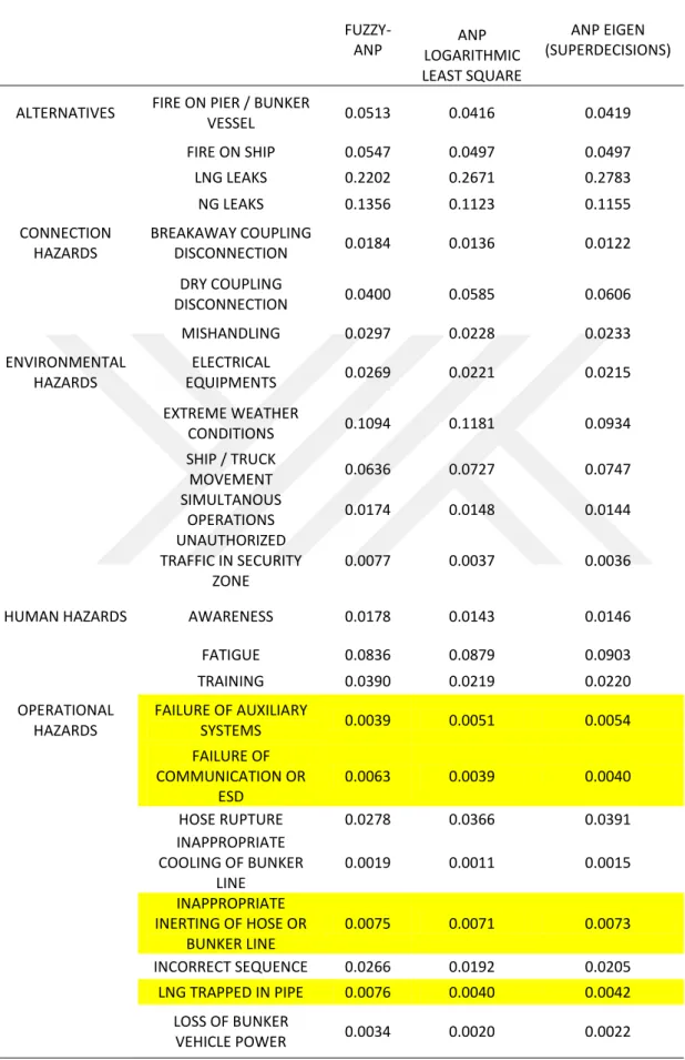
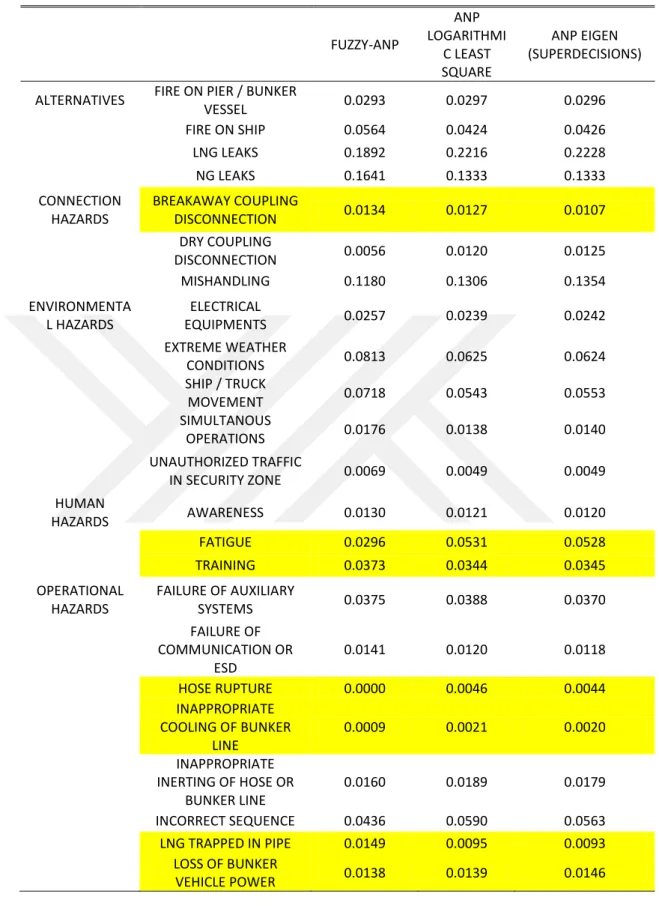
As result LNG leaks have been found the most critical risk alternative for all calculation methodologies.

(23)

DENĠZ YAPILARI ĠÇĠN GÜVENLĠK TABANLI KARAR DESTEK SĠSTEMLERĠ ÖZET

Dünya yüzeyinin %71’i suyla kaplıdır ve insanlık tarihinin gelişimi boyunca insan bir şekilde suyla mücadele ederek ilerleme kaydetmiştir. Bu sayede medeniyetlerini yaymış, ticareti arttırmış ve gelişmeyi sağlamıştır. Olasılık teorisinin başarıyla çalıştığı ve risk alarak başarıya ulaşılan pek çok yer olabilir ancak tarihsel veriler şünu göstermektedir ki, denizcilik sektörü bunlardan birisi değildir. Alınan küçük risklerin çok büyük felaketlere sebep olduğu defalarca görülmüştür. Yaşanılan büyük kazalar sonrası alınan tedbirler ve Uluslararası Denizcilik Örgütü’nün kaza analizleri sonrası ortaya koymuş olduğu kural ve kaideler, insanoğlunun deniz ile mücadelesinde kazanımlar sağlamış olmasının en önemli nedenidir.

Risk analizi belirsizlikler ile başa çıkmak için önemli ve çok güçlü bir araçtır. Yeni teknolojiler, yeni gelişmeler ve yeni metodolojiler her zaman belirsizlikleri ve böylece riskleri içerir. Bu risklerle başa çıkmak için birçok farklı yöntem vardır. Niteliksel ve niceliksel yöntemler pek çok farklı sektörlerde başarı ile yıllardır kullanılmaktadır. Kantitatif çalışmalar daha fazla istatistiki verilere ihtiyaç duymaktadır. Analizlerde hem sayısal hem de sözel verilerin kullanılabilmesi projenin herhangi bir aşamasında risk analizi gerçekleştirmenizi sağlar. Tehlike Tanımlama (HAZID) ve Tehlike ve İşletilebilme (HAZOP) çalışmaları, güçlü ve yaygın olarak kullanılan analiz yöntemlerindendir. Bu çeşit çalışmalarda uzmanlardan oluşan bir grup riskleri tanımlamak ve olası riskleri değerlendirmek için çaba harcarlar. Grup içerisinde bir veya daha fazla katılımcı karar verme mekanizmalarında hakimiyete sahip olursa, bu tarz çalışma grupları sorunlu olabilir. Ve genellikle grup içerisinde konu hakkında baskın fikir birliği sebebiyle tanımlara belirsizliği dahil etmek zordur. Buna ragmen oldukça sık kullanılan bu yöntemler ile pek çok denizcilik uygulamasının risk değerlendirilmesininde karşılaşılmaktadır.

Riski tahmin etmek yeni sistemlerin analizi için hayati öneme sahip bir fonksiyondur. Tahmin sistemi üç aşamadan oluşmaktadır; riski tanımlar, riski analiz etme ve riski ortadan kaldırma. Bunlardan ilki riski tanımlama “ne zaman, ne, kim, nasıl ve nerede” sorularının cevaplarının aranmasıyla başlar. Bunlara cevap bulunup tanımlama işlemi tamamlandığında ikinci kısma yani analiz kısmına geçilir. Analiz bir derece daha olaya odaklanmıştır ve “ne kadar, ne sıklıkta ve ne kadar önemli” sorunlarının cevaplarını elde etmeyi amaçlar. Alınan cevaplar, analizi yapana riskin doğasını sıklığını ve seviyesini anlama imkanı sağlar. Analiz tamamlandıktan sonra, belirlenen riske karşılık ne tedbir alınacağının kararlaştırılması safhasına geçilir, bu safha değerlendirme safhasıdır. Bu aşamada analiz safhasında tespit edilen riskin etkisini düşürmek amacıyla neler yapılması gerektiği kararlaştırılır; riskin etkisine bağlı olarak karşı tedbir almamak veya riski bir sigorta firmasına transfer etmek de uygulanabilecek yöntemlerdendir.

Risk yönetimi için kullanılabilecek, ISO standartlarında tanımlanmış çeşitli teknikler mevcuttur. Standartta yaklaşık 30 farklı teknik tariflenmiştir. Hangi method kullanılırsa kullanılsın, karar vericilerin konuya hakimiyeti, bilgileri ve riske bakış açıları sonucu doğrudan etkileyecektir. Doğru bir analiz sonucu elde edebilmek için sorun her bakış açısından dikkatlice incelenmelidir. Başarı metodolojiye bağlı

(24)

olmasına ragmen, tüm analiz yöntemlerinin tek ortak ana parçası insandır ve sonucu doğrudan etkilemektedir.

Farkında olunsun ya da olunmasın, karar verme seçimleri ile her gün günlük hayatta karışılaşılmaktadır. Saaty Analitik Hiyerarşi Proses (AHP) ile karar verme problemlerini çözmebilmek için Eigen vektörlerini kullanılmanın mümkün olduğunu kanıtladı. Bu çalışması ile Saaty, yeni çalışmalara ve yöntemlere kapıyı aralamıştır. Pek çok başarılı uygulaması olmasına ragmen, gerçek problemleri hiyerarşik bir yapıda modelleme konusunda zorluklar, AHP kullanımını kısıtlamaktadır; bu sebeple Saaty bağımlılıkları ve geri bildirimi ile ağ yapısında bir modelleme yöntemi geliştirmiştir. Bu metodoloji Analitik Ağ Süreci (ANP) diye adlanrılmıştır. ANP başarılı bir şekilde karmaşık karar verme problemlerini modelleyebilmektedir. Ancak modelleme ve modelin çözümü AHP’ye kısayla çok fazla sabır ve çaba gerektirmektedir. Zira ağ modelin her bir bağlantısı için ikili karşılaştırma yöntemi kullanılması gerekmektedir. Bunun dışında bulanık küme teorisinden faydalanılarak, bulanık çok kriterli karar yöntemlerini (fuzzy) kullanmak, ANP’nin çözümlerine bulanık ortam etkilerini katmak için alternatif bir yöntem olarak tavsiye edilmiştir. Belirsizliği içeren bulanık kümeleri her türlü soruna uygulamak kolaydır. Bulanık setlerde de bazı zorluklar vardır. Bulanık küme tanımların yapılabilmesi için, üyelik fonksiyonlarını tanımlak da tecrübe gerektirir. Tanımlanmış kuralları da değiştirmek o kadar kolay da değildir, dolayısıyla system baştan detaylı düşünülmeli ve ona gore düzenlenmelidir. Bu tür sebeplerden dolayı nispeten uygulaması daha kolya olan Bulanık-AHP, Bulanık-ANP, vb. hibrid yöntemlerin kullanılması yaygındır. Pek çok hibrid çözüm metodolojileri geliştirilmiştir, böylece uygulayıcı, probleminin doğasına uygun olan yöntemi doğrudan seçip kullanabilir.

Bu çalışmada, LNG yakıt dolum operasyonu vaka çalışması olarak seçilmiştir. LNG mevcut yakıtlar arasında, Uluslararası Denizcilik Örgütü ve bir takım ülkelerin hava kirliliği ile mücadele kapsamında koymuş olduğu kurallara uyabilecek en olası alternatiflerden biridir. Yakıt dolumu LNG kullanımı işleminin en riskli parçasıdır. Yakıt dolumu ile ilgili HAZID / HAZOP çalışmaları, klas kuruluşlarının yakıt dolumu ile ilgili geliştirdileri prensipleri yakıt dolumu için olabilecek tehlikelerin tanımlanmasında kullanılmıştır. Tehlikeler ve riskler Hata Ağacı Analizi (FTA) kullanarak kümeler altında toplanmıştır ve bu kümelerden ANP ağ yapısı oluşturulmuştur.

Oluşturulan ANP ağ yapısı; ANP (logaritmik en küçük kareler) ve Bulanık-ANP yöntemleriyle çözülmüştür. Bu çözümler için eklerde sunulan excel kodları yazılmıştır. Bulanık-ANP çözümü için, pek çok geliştirilmiş olan çeşitli metodolojiler bulunmaktadır, çözüm için bunlardan bir tanesi kullanılmıştır.. Bu çalışmada bulanık ortam modellemesi için üçgen bulanık fonksiyonlar kullanılmıştır ve bunlar için Chang’ın geliştirmiş olduğu yöntem çözüm olarak kullanılmıştır.

Elde edilen sonuçları doğrulamak amacıyla “Superdecision” isimli programda aynı ağ yapısı oluşturulmuş ve program ile Eigen değerleri kullanılarak ANP çözümü elde edilmiştir. Elde edilen çözüm bulanıklık faktörünü içermemektedir. Tüm çalışmanın sonunda yapılan hesaplamalar ile çalışmada aynı ağ yapısı için üç farklı yönteme dair sonuçları karşılaştırma şansı elde edilmiştir.

Yapılan tüm hesaplamalardan sonra risk değerlerinin hesabı için; riskin gerçekleşme ihtimali ve olası sonuçlarının çarpımı hesapta kullanılmıştır.

Çalışmaya altı adet uzman davet edilmiştir, bunlardan iki tanesi klas kuruluşunda görevli, iki tanesi armatör firmada lng operasyonlarında çalışmış ve diğer iki tanesi ise lng sistemleri üreten bir firmada çalışmaktadırlar. Davet edilen tüm uzmanlar lng konusunda kendi bölümlerinde çalışmaktadırlar. Davet edilen uzmanlardan iki tanesi daveti olumlu cevaplandırmıştır. Bu uzmanlardan, oluşturulmuş olan ANP ağ yapısına göre önceden tanımlanmış anketleri doldurmaları istenmiştir. Her bir karar

(25)

verici için elde edilen final sonuçlar, Bireysel işlemlerin kümeştirilmesinde kullanılan AIP yöntemi ile tek bir karar vericiye indirgenmiştir.

Karar vericilerin kararları sonuç için birleştirilirken her bir karar vericinin sonuç üzerinde aynı derecede etkisi olmadığı yani ağırlıklarının farklı olduğu varsayılmıştır. Bu da her bir kullanıcı için elde edilen farklı ağırlıklar kullanılarak aynı yöntem içerisinde çözülmüştür. Karar vericilerin ağırlıklarını hesaplayabilmek için ufak bir ayrı ANP yapısı oluşturulmuş ve bu yapı çözülerek her bir karar vericinin ağırlığı elde edilmiştir.

ANP yapısının her bir küme ve küme elemanı için sonuçları incelendiğinde; ANP (logaritmik en küçük kareler yöntemi) ile ANP (Superdecisions) sonuçlarının birbirlerine çok yakın olduğu görülmektedir. Bunun sebebi Saaty ve Vargas’ın 1984 yılındaki çalışmalarında belirttikleri gibi muhtemelen tutarlılık oranının 0.1’in altında tutulmuş olmasından kaynaklanmaktadır. Daha büyük tutarlılık oranlarında çalışma tekrarlanıp değişim incelenebilinir. Ancak 0.1 altındaki değerlerde sonuçlar birbirine çok yakındır.

Bulanık-ANP sonuçları, logaritmik en küçük kareler ve eigen değerleri ile hesaplanan ANP sonuçlarından biraz farklılık göstermiştir. Ancak gözüken farklılık sonucu değiştirecek derecede büyük değildir. Bulanıklık fonksiyonların kullanılmasının sebebi bu farklılığın görülmesidir, ki bu beklenen bir sonuçtur. Burada dikkat edilemesi gereken bulanıklığın sonucu ne kadar oranda değiştirebildiğidir. Yapılan uygulamada üçgen bulanık fonksiyonlar kullanılmıştır, ileriki çalışmalarda daha farklı fonksiyonlar ile yeni hesaplamalar yapılarak diğer yöntemlerdeki sonuçlar ile olan farklılıklar karşılaştırılabilinir.

Yapılan çalışmalarda LNG kaçaklarının diğer belirlenmiş olan risk alternatiflerine gore daha tehlikeli olduğu gözükmektedir. Bunun sebebi LNG kaçaklarının diğer kaçak ve yangın risklerini içerisinde barındırmasından kaynaklanmaktadır.

(26)

(27)

1 INTRODUCTION

Our planet’s 71% of the surface is covered by water. One of the main targets of the human being for development has always been dealing with the sea. There are places for gambling or taking a bit of a risk where probability theory works fine, but for sure the sea is not one of them. It is obvious that the sea is not a place for human to live and maritime history is full of many preventable catastrophic accidents. However historical evidences, beside all those accidents and failures, prove that human challenge the sea for a very long time with a remarkable success. This has been achieved by taking lessons from the failures and accidents.

Primary objective in marine industry has always been to select the lowest cost alternative, but the trends have changed towards the trade-off among safety, cost, environment and technical performance. The last decade many environmental regulations have entered into the force for maritime transportation and many are prepared for the next decade. Air pollution is one of the main environmental items, there is a couple of “Emission Control Area (ECA)”s around the world and many new of them are on the agenda. Using conventional marine fuels such as Heavy Fuel Oil (HFO), Marine Diesel Oil (MDO) in most of the ECA ports is forbidden, instead new MDO with low sulfur content has already been in the market for a while. New rules and regulations put into the force new restrictions on fossil fuels. Liquefied Natural Gas (LNG) has come up as a good and applicable solution for marine transportation. LNG is a cheaper and environmental friendly solution beside current marine fuel types. LNG has already been used for decades as marine fuel in big LNG carriers, by using their own cargo’s boil-off gases, those ships normally perform their loading and discharging operations away from public life. However, using LNG in other type of ships, travelling all around the ports close to public life, is a new challenge for public, governments, International Maritime Organization (IMO), classification societies, designers and ship owners. As per IMO “International convention for the safety of life at sea” using fuels with low flashpoints are prohibited. After many research projects, in 2015, IMO Maritime Safety Committee (MSC) adopted new “International Code of Safety of Ships Using Gases or Other Low Flashpoint Fuels” (IGF Code), expected to enter into the force on 1sth of January, 2017 with new SOLAS amendments. However, several ships are sailing in

(28)

international waters and many of them are under construction with special exemptions from flag authorities using LNG or dual-fuel (LNG and HFO/MDO). Specific risk study methods have been applied to convince the flag authorities. Risk studies are very well known and often used in offshore industry, however marine industry is not very familiar with them. Most of the classification societies have rules, regulations and guidelines to implement risk based inspection techniques, unfortunately they are rarely used during ship inspections.

It is quite clear that LNG will be the future fuel for marine transportation and marine industry, therefore the systems for LNG should be developed according to the new conditions. In 2016 three oil/chemical tankers, one asphalt carrier and two roll on – roll off ferries with dual-fuel engines are under construction in Turkiye. With the permission and attendance of the flag authority representatives, hazardous identification (HAZID) and hazard and operability studies (HAZOP) have already been performed. According to those studies it has been concluded that the most challenging part of using and carrying LNG is the bunkering.

1.1 Scope and Limitations

Based on the risk studies; “LNG bunkering operation” is selected as the risk problem for this study. Six experts (2 from LNG systems manufacturer company (Italy), 2 experts from classification society (France), 2 owner representative (Canada)) who have experience on LNG systems on board and have attended the LNG studies for ongoing projects, are asked to participate. HAZID/HAZOP study results are present as group decision, the risk items are not exactly unique however by using questionnaire for each expert, it has been also possible to observe the difference between the group’s and each individual experts’ decision. Due to the limited statistical data, qualitative risk analysis method is used to review the problem. Fuzzy-Analytical Network Process (ANP) decision making method is chosen to calculate the priorities of experts and aggregate the total solution.

There may be three cases for bunkering operation, those are;

 Ship to ship transfer

 Truck to ship transfer

 Shore facility to ship transfer

Ship to ship LNG transfer is a new concept and needs some more time to develop new rules and regulations. Today there are very limited number of LNG bunkering (ship to ship) vessels under construction. LNG transportation and LNG

(29)

loading/discharging from shore facility has been done for decades and it has already proved its reliability. Today most of the LNG bunkering for non LNG carriers are done by trucks. That is why, truck to ship transfer bunkering case is considered in this study.

Several decision making methods examined and fuzzy-ANP method has selected. ANP is a reliable method to model complex problems while fuzzy sets are flexible for defining pairwise comparisons.

(30)

(31)

2 LITERATURE REVIEW

Decision making is not only human problem that everyday can be faced all life forms and decision making results people to live or die. Historically, human decision theories have focused on outcome prediction. Modern decision making is based on; understanding of decision making processes, thoughts and application of technology tools to support process by human beings.

In earlier times, society leaders consulted their elders for the result of choices, elders replaced by the fortune tellers, wizards, astrologists, religious figures in time and nowadays they may be called as manager consultants. People used dices, bones, stones and many other objects to predict the results of their choices. Julius Caesar’s famous words, taken from Menander (Greek comedy writer), “the die is cast” or may be a better translation “the die has been cast” on his armies way to Rome before they pass the River Rubicon (Tranquillus, AD 121). He selected his choice from his alternatives, most probably it was checked by his dices and now die is cast and fortune is set. Dices luckily is not needed as well as bones, fortune tellers or any other figures. The better decisions can be made by couple of researchers and thousands of applications.

2.1 Risk Management

ISO 31000 Risk management – Principles and guidelines; is a standard to provide principles for managing risks (ISO, 2009). According to this document, risk is the effect of uncertainty on objectives and risk management is the coordinated activities to direct and control an organization with regard to risk.

The main element of risk management is stakeholders; communicating and consulting stakeholders is generally done by using brainstorming, Delphi or similar methodologies in order to increases the efficiency of the process. Managing risk starts with scope and context definition, this stage draws the borders of the study, includes internal and external contexts. After finalizing scope definition, risk assessment is the next stage that is defined in detail under Section 2.2. Risk treatment is the last step of risk management, uses the output of risk assessment, especially risk matrix. Treatment stage is decision stage, here results of analysis are

(32)

compared to the risk criteria. Risks may be positive or negative, depending on the nature of the system.

Risk management process should be monitored and reviewed in time, to eliminate new emerging risks.

Ineffectual methods may even be touted as “best practices” and, like a dangerous virus with a long incubation period, are passed from company to company with no early indicators of ill effects until it’s too. Main question is; would anyone in the organization even know if risk management method didn’t work? A weak risk

Figure 2.A:Risk Management Steps. DEFINE SCOPE, CONTEXT RISK IDENTIFICATION RISK ANALYSIS RISK EVALUATION RIS K A S S E S S M E NT RIS K M A N A G E M E NT LIKELIHOOD CONSEQUENCE RISK LEVEL RISK TREATMENT RISK RESULT CO MM UNI CA T IO N, CO NS ULT A T IO N RIS K A C CE P T A NCE CRIT E RI A

(33)

management approach is effectively the biggest risk in the organization (Hubbard, 2009). That is why, the risk management process has to be tailor made in order to cope with each particular case and project in an organization. Best practices are not always, even good ones.

2.2 Risk Assessment “Risk is a construct, before risk there was fate” (Bernstein, 1996). During the

transformation from ancient to the modern world; fate has transformed to a calculable value in terms of risk. Today risk may be defined as potential of gaining or losing something in value and because of this potential is uncertain, it may also be

defined as measurable of uncertainty. Life itself is full of uncertainty, in every single moment of life, decisions are being

made to shape the life itself. Risks are not always negative, there may be some cases, especially in marketing or financial business, for positive risks, because the nature of these risks include hazards and opportunities at the same time. In this study only negative risks are dealt with. Understanding the risks, by using risk assessment is the main step of managing the risk. ISO/IEC 31010:2009 Risk management – Risk assessment techniques is a supporting standard for ISO 31000 Risk management – Principles and guideline. ISO/IEC 31010:2009 is a generic risk management standard, containing guidance on how to select and apply systematic techniques for risk assessment. This document contains more than 30 techniques, some are; brainstorming, interviews, checklists, Structured what-if technique (SWIFT), scenario analysis, fault tree analysis, bow tie analysis, Delphi method, Hazard and operability study (HAZOP), Failure mode and effects analysis (FMEA), event tree analysis, cause and effect diagrams, human reliability analysis, Monte Carlo simulation, risk index etc.

The success is methodology depended, however the main component of all analysis methods is human. Whatever the method is used, knowledge of experts, their understanding of problem and their position to view the risk will directly affect the result. In order to get proper assessment results, problem has to be thought from all sides of aspect.

The reason of the importance of the design of the solution set is not only because of the human factor but also modeling the reality of the problem. The model shall reflect the truth and based on the model, the chosen method shall reflect the true decisions of the decision makers.

(34)

Risk assessment consists of three main parts as shown in Figure 2.B.

Questions that define risk assessment items are also shown in Figure 2.C.

2.2.1 Risk identification

Risk identification phase tries to recognize and record risks by asking them main question “what might happen?”. After the answer is given to the main question, causes and sources of risks are identified by using other questions mentioned in Figure 2.C. Evidence methods such as historical data, checklists, expert methods such as brainstorming, Delphi or inductive reasoning techniques such as HAZOP, Primary hazard analysis (PHA), event tree, etc. All these methods may all be used depending on the nature of the problem.

A table of risk assessment techniques based on ISO/IEC 31010:2009 Risk management – Risk assessment techniques, which may be applied for risk identifications is listed as Table 2.1. Table indicates the methods as “strongly applicable” and “applicable”.

Risk Identification

Risk Analysis

Risk Evaluation

Figure 2.B: Risk Assessment.

Why, How often, How much, How critical,

Level of risk based on what criteria

What is acceptable or unacceptable, Solution options, priorities Risk Identification

Risk Analysis

Risk Evaluation

What, Who, When, Where, How

(35)

Table 2.1: Risk identification methods.

Methods listed as “strongly applicable” by the standard

 Brainstorming

 Structured or semi-structured interviews  Delphi

 Checklists

 Primary hazard analysis  Failure mode effect analysis  Reliability centered maintenance  Consequence/probability matrix

 Hazard and operability studies (HAZOP)  Hazard analysis and critical control points (HACCP)

 Environmental risk assessment  Structure what if (SWIFT)  Scenario analysis

 Cause and effect analysis  Human reliability analysis

Methods listed as “applicable” by the standard

 Business impact analysis  Fault tree analysis  Event tree analysis

 Cause and consequence analysis  Layer protection analysis (LOPA)  Sneak circuit analysis

 Markov analysis  FN curves  Risk indices

 Cost / benefit analysis

 Multi-criteria decision analysis (MCDA)

2.2.2 Risk analysis

Risk analysis is the second phase of risk assessment, helps us to develop and understand risk. Nature, sources and causes of risks are analyzed in order to define or estimate the level of consequence and likelihood for each defined risk hazard. Each consequence and likelihood are then combined to define the level of risk. Analysis may be done by qualitative, semi-quantitative or quantitative methods, method should be selected depending on the nature of the problem and available data. Different methods may be used to define likelihood, consequence and level of risk. As an example; fault tree analysis may be used while defining likelihood, while consequences may be defined by FMEA.

At the end of the analysis phase, the strength and weakness of the system and process will be defined.

2.2.3 Risk evaluation

In evaluation phase, risk criteria, defined at the beginning within context, is compared with risk level results from risk analysis phase. Risk is understood in analysis phase and in evaluation phase decisions for future action is made. Main item to decide is; whether risk level need treatment or not. Cost - benefit analysis (CBA) or more detailed Benefits, opportunities, costs, risks (BOCR) analysis are used to support the decision. It is usually not cost-effective to treat all risks that is why prioritization of chose treatments is needed. Risk evaluation is the last step of

(36)

risk assessment, output of this phase are; risk levels and items to be treated including their priority order. Choice will be done in next step, risk treatment section. 2.3 Risk Treatment

Risks are not always negative, there may be some cases that risks may cause opportunities, however in this study only negative risks are considered. List of items that needs to be treated, their priority order are inputs coming from risk assessment and risk criteria defined within the context, at the beginning of the study is another input for this phase. Selected treatment alternatives based on agreement of the experts are to be implemented. Treatment of risks can be done by one of the following four methods;

 Accepting risk; done by taking no action. In this method risk and it’s consequences accepted. Generally performed for small risks.

 Avoiding risk; for major risks, changing the game plan to avoid the defined risk is one of the best way to follow.

 Transferring risk; not used commonly. Idea is to transfer the impact and management of risk to someone else, insurance is a good example for this method.

 Mitigating risk; the most common way to deal with risks. Taking precautions to reduce the likelihood or severity of loss is all risk mitigation.

2.4 Multiple Criteria Decision Making Methods

Decisions made draw the path of life, decisions shapes the life. Every decision has its own consequences. There are many decision making methods in the open literature.

Multiple criteria decision analysis is a discipline that finds solution to the problems structured on multiple criteria. Depending on the nature of the problem one of the two sub-disciplines of Multiple criteria decision analysis (MCDA) has to be used, these are;

 Multi attribute decision making (MADM)

 Multi objective decision making (MODM)

Multi attribute decision making deals with the problems that makes decision among some pre-defined alternatives in the presence of multiple, generally conflicting attributes.

(37)

Multiple objective decision making deals with the design problems that cope with finding the best alternative by considering a set of interacting design constraints, no decision alternative is present in the model which also means number of alternatives is effectively infinite.

Multi attribute decision making is the most well-known branch of multiple criteria decision making method. MADM problems are assumed to have a predetermined, limited number of alternatives. Solving a MADM problem involves in sorting and ranking of alternatives.

Some of the MADM methods are; Maximin, Maximax, Weighted Product, Technique for order of preference by similarity to ideal solution (TOPSIS), Elimination et choix traduisant la réalité (ELECTRE), Analytical Hierarchy Process (AHP), Analytic Network (ANP), etc.

One of the first critical work about decision making was published by Saaty (1977). In this paper, method of scaling ratios using the principal Eigen vector and pairwise comparison matrix is described. Consistency of the matrix data is defined and measured by an expression involving the average of the non-principle Eigen values. 1 to 9 scale numbers are introduced together with a discussion of how it compares with other scales. Application of some examples for which the answer is known, presented for validating the approach. The hierarchy of multiple criterion decision making, properties of hierarchies and the Eigen value approach application to scaling hierarchically structured complex problems are also presented in this study. Saaty and Vargas (1984) published two different papers about dealing with the inconsistency and rank reversal situations. In these studies conditions for rank preservation in a positive reciprocal matrix that is inconsistent are provided and three methods; the Eigen value, the logarithmic least squares, and the least squares, examined to derive estimates of ratio scales from a positive reciprocal matrix. It is shown that only the principal Eigen vector directly deals with the question of inconsistency and captures the rank order inherent in the inconsistent data.

Another game changing method has also been presented by Saaty (1996), in this study, instead of hierarchical structure a network system used to define the decision problem.

(38)

Table 2.2: List of main AHP/ANP Studies.

Year Researcher Concept of the study

1977 T.L. Saaty

Method of scaling ratios using the principal Eigen vector, pairwise comparison matrix is described and

consistency of the matrix data is defined

1979 B.G. Merkin

Defines mathematical structure of consistent matrices and eigenvector's ability to generate true or

approximate weights

1980 T.L. Saaty The Analytical Hierarchy Process defined 1984 T.L. Saaty &

L.G. Vargas

Comparison of Eigenvalue, Logarithmic Least Squares and Least Squares Methods in Estimating Ratios 1984 T.L. Saaty &

L.G. Vargas Inconsistency and Rank Preservation 1986 T.L. Saaty Axiomatic Foundations of the Analytical Hierarchy

Process

1987 T.L. Saaty Rank Generation, Preservation and Reversal in the Analytical Hierarchy Decision Process 1996 T.L. Saaty The Analytic Network Process defined 1998 T.L. Saaty &

L.G. Vargas Bayes’ Theorem and the Analytical Hierarchy Process 2003 T.L. Saaty

Dynamic decision making; defines using functions for the paired comparisons and derive functions from them.

This describes a new powerful tool. 2005 _{M.S. Özdemir}T.L. Saaty & Dictionary of Decisions using ANP 2009 T.L. Saaty & B.

Cillo Dictionary of Complex Decisions using ANP

In the study named “Fuzzy Sets”, Zadeh (1965) introduced fuzzy sets as an extension of the classical notion of sets. Later this idea is used in many methods to model and solve fuzzy problems. Zimmerman, Zadeh and Gaines (1984), Zimmermann (1986, 1987) issued studies about using fuzzy sets in decision making problems. Using hybrid methods idea first came up with Van Laarhoven and Pedrycz (1983) triangular membership functions used to describe fuzzy ratios which have been used to make comparisons in AHP. Buckley (1985), Mon and Cheng (1985) and Chang (1986) introduced formed important methodologies to solve hybrid fuzzy AHP problems.

(39)

In Table 2.3 some of the important fuzzy and fuzzy AHP/ANP hybrid studies are listed.

Table 2.3: List of Fuzzy Logic and Fuzzy-AHP/ANP Studies.

Year Researcher Concept of the study

1965 L.A. Zadeh Description of fuzzy sets

1970 R.E. Bellman & L.A.

Zadeh Decision making in a fuzzy environment 1977 M.S. Baas & H.

Kwakernaak

Rating and Ranking of Multiple-Aspect Alternatives Using Fuzzy Sets 1978 R.R. Yager Mathematical solution method for fuzzy 1978 W.J.M. Kickert Fuzzy theories to use for decision making

1983

P.J.M. Van Laarhoven &

W. Pedrycz Adopting fuzzy methods for Saaty’s theory 1984 H.J. Zimmermann & L.A.

Zadeh & B.R. Gaines

Use of fuzzy sets in decision making analysis

1985 J.J.Buckley

Method to use fuzzy ratios instead of exact ratios in AHP, uses geometrical mean to

calculate mean fuzzy ratios 1986 H.J. Zimmermann Solving fuzzy set models for crisp

environments

1987 H.J. Zimmermann Extend of his previous issue 1995 D.L. Mon & C. Cheng Definition and application of Cheng’s

method for fuzzy AHP problem 1996 D.Y. Chang Definition and application of Chang’s

method for fuzzy AHP problem In this study ANP and hybrid fuzzy model fuzzy-ANP are described and used. 2.4.1 Pairwise comparison

Pairwise comparisons using ratio scales was developed by Saaty (1980). According to Saaty’s study decision problems are structured into smaller parts in a hierarchical structure and each small structure is handled by pairwise comparison matrices. Pairwise comparisons are always a more precise way of establishing priorities for alternatives than rating them at once and real data and statistics representing probabilities and likelihood can also be used in relative form instead of making pairwise comparisons in the ANP as they are in AHP (Saaty,2005). The

(40)

mathematician and cognitive neuropsychologist Stanis Dehaene states in his book “The number of sense, how the mind creates mathematics” that introspection suggests that we can mentally represent the meaning of numbers 1 through 9 with acuity (Saaty, 2005). Table 2.4 indicates the comparison scale with definition. These symbols seem equivalent to us and this makes them easy to work with. However there may be a problem in pairwise comparisons; inconsistency. In life, inconsistency helps us to change our minds in case a new information that contrast with previously known consistent knowledge. This helps the human to move forward. Unfortunately too much inconsistency unsettles human thinking. According to Saaty this means that; inconsistency must be large enough to allow for change in our consistent understanding, but small enough to make it possible to adapt our old beliefs to new information. 10% of the total concern with consistent measurement will provide enough inconsistency for pairwise comparisons. Calculation of inconsistency is described under Section 2.4.3.

Pairwise comparisons are always a more precise way of establishing priorities for alternatives that rating them one at time (Saaty, 2005).

Table 2.4: Fundamental Scale for Pairwise Comparison. Intensity of

importance Definition

1 Equal importance between two objectives

3 Moderate importance of one objective over the other 5 Strong importance of one objective over the other 7 Very strong importance of one objective over the other 9 Extreme importance of one objective over the other 2, 4, 6, 8 Intermediate values

2.4.2 Solving matrices

Different methods have been defined to solve pairwise comparison matrices. Saaty (1977) defined a method to solve the pairwise matrix, eigenvectors are suggested. It is concluded that if inconsistency is allowed in a positive reciprocal pairwise comparison matrix, the principal eigenvector is necessary for representing the

(41)

priorities associated with that matrix, providing that the inconsistency is less than or equal to a desired value (Saaty, 2003).

Suggested methods for solving matrices are listed as follows;

 Eigenvector method

 Least squares method

 Logarithmic least squares method

Saaty and Vargas (1984) presented a study for comparing the results of these methods. It is concluded in this study that when consistency obtains, three methods produce identical solutions, however when there is inconsistency in the data, the best solution is to use eigenvector method. In order to use other methods mentioned either inconsistency should be accepted or reduced by improving the quality of information as described under Section 2.4.1.

2.4.3 Dealing with inconsistency

In reality consistency helps us to change our minds in terms of new information. Too much consistency is undesirable because we are dealing with human judgments. Evaluation of rating inconsistency is done by calculating Consistency Ratio (CR), to measure how consistent the judgments have been relative to large samples of purely random judgments which are calculated and indexed by Saaty (1980) given in Table 2.5. In order to calculate CR, Consistency Index (CI) is divided by mean random CI.

[1]

is the maximum eigenvector of pairwise comparison matrix and is the size of the matrix then the CI is calculated as below:

[2]

Table 2.5 represents the mean random consistency index values calculated by Saaty, first row represents the size of the matrix while second row is the corresponding index of consistency for random judgments.

(42)

Table 2.5: Mean Random Consistency Index.(Saaty, 1980)

3 4 5 6 7 8 9 10 11 12 13 14

0.58 0.9 1.12 1.24 1.32 1.41 1.45 1.49 1.51 1.48 1.56 1.57 Saaty(1980) represents the acceptable threshold value for CR as 0.10, according to his studies values over this threshold values indicates that comparison is inconsistent and has to be re-evaluated.

In a complex system having too many pairwise comparison may result to lose the consistency. Psychologists suggest to ranking criteria before making pairwise comparison, and believe that this might reduce inconsistency.

2.4.4 Rank reversal

Rank reversal phenomenon occurs when a decision maker, makes decision from a set of alternatives and, is confronted with new alternatives that were not thought about when the selection process was initiated. For instance three alternatives are considered in a decision making problem; X, Y, Z. And according to pairwise comparisons it has been figured out that X is better than Y, Y is better than Z. If a new alternative, T, which is not better than Z is replaced with alternative Y, it has been observed that under some circumstances the previously ranked as best alternative X, is not still the best one. This condition is known as rank reversal, this example only describes one type of rank reversal, there are some others in the literature.

Decision making community has no consensus on rank reversal, whether or not it shall be prevented.

There are two different modes used in common;

 Ideal mode using weighted product method

 Distributed Synthesis mode using weighted sum method

Ideal mode introduced by Forman (1993) as an alternative synthesis to Saaty’s original AHP which is proved that allowing rank reversal.

2.4.5 Group decision making

In group decision two things may happen, either members engage in discussion to get a consensus or express their own preferences. These conditions are named, in order;

(43)

 Aggregation of individual judgments (AIJ)

 Aggregation of individual priorities (AIP)

When synthesizing the judgments of n judges below listed conditions shall be considered.

 Pareto principle (unanimity condition); if members of a group prefers alternative A to B, then the synthesized judgment shall prefer A to B.

( )

[3]

 Homogeneity condition; if each members of a group judge a ratio Y times as big as another ratio, then the synthesized judgment shall also be Y times bigger.

(

) (

)

[4]

Where

 Reciprocity requirement; synthesized value of the reciprocal of the individual judgments shall be the reciprocal of the synthesized value of the original judgments.

(

)

(

)

[5]

Aggregation of individual judgments (AIJ);

If the group members are not willing to act on their own preferences and instead members are willing to pool their judgments, then the group becomes a new individual and behaves like one, having a common decision. Thus, Pareto principle is irrelevant. Since the group becomes a new individual and behaves like one, the reciprocity requirement for the judgments has to be satisfied, in that case geometric mean must be used instead or arithmetic mean.

In that case, each group member performs own pairwise comparison then using the below formula, a unique group matrix and priorities vector are produced. By solving this matrix solution for the group decision has been found.

(44)

, -

∏(

)

[6] , -

∏ .

, -

/

[7]

, - the group matrix number of group members

* +

is matrix size

pairwise comparison matrix of “k”th member is weight of the “k”th group member

, -_{group priority vector}

Aggregation of individual priorities (AIP);

If the group members are willing to act on their own preferences without pooling their judgments. In this case the problem is solved for each member individually to get their own priorities. Both arithmetic and geometric means may be used, neither method will violate Pareto principle. Formulation is given below.

, -

∏ .

, -

/

[8] , -

∏(

)

[9] ,

group priority vector, number of group members,

* +

is matrix size

pairwise comparison matrix of “k”th member, is weight of the “k”th group member

,

priority vector of “k”th member

Geometric and arithmetic means with expert weights;

f(X) is the decision function, subscript A and G represents arithmetic and geometric means in order, is the expert weight, n is the number of experts and Xi is the

(45)

decision of each expert. Arithmetic and geometric means with expert weights are calculated as given below.

∑

[10]