Damping of Electromechanical
Oscillations in Power Systems using
Wide Area Control
Von der Fakultät Ingenieurwissenschaften der Universität Duisburg-Essen
zur Erlangung des akademischen Grades eines
Doktor der Ingenieurwissenschaften (Dr. -Ing.)
genehmigte Dissertation von
Ashfaque Ahmed Hashmani
ausMatiari, Pakistan
Referent: Prof. Dr.-Ing. habil. István Erlich Korreferent: Prof. Dr.-Ing. S. X. Ding Tag der mündlichen Prüfung: 15.07.2010
Acknowledgment
I am grateful to my supervisor Prof. Dr.-Ing. habil. István Erlich for his sup-port and invaluable suggestions throughout my Ph.D. study. He treats all his students equally. This gave me courage to work here, away from my home-land.
I would also like to thank all the members of the Institute, for their corpo-ration.
Finally, I would like to thank the Deutscher Akademischer Austausch Di-enst (DAAD) and Higher Education Commission (HEC), Pakistan for spon-soring my Ph.D. study at the Institute of Electrical Power Systems, University of Duisburg-Essen, Germany.
Last, but not least, my gratitude goes to my wife, mother and father. With-out their encouragements and continuous support this Ph.D. study could not have come to a satisfactory conclusion.
Abstract
The design of a local H∞-based power system stabilizer (PSS) controllers,
which uses wide-area or global signals as additional measuring information from suitable remote network locations, where oscillations are well observ-able, is developed in this dissertation. The controllers, placed at suitably se-lected generators, provide control signals to the automatic voltage regulators (AVRs) to damp out inter-area oscillations through the machines’ excitation systems.
A long time delay introduced by remote signal transmission and processing in wide area measurement system (WAMS), may be harmful to system stabil-ity and may degrade system robustness. Three methods for dealing with the effects of time delay are presented in this dissertation. First, time delay com-pensation method using lead/lag comcom-pensation along with gain scheduling for compensating effects of constant delay is presented. In the second method, Pade approximation approach is used to model time delay. The time delay model is then merged into delay-free power system model to obtain the de-layed power system model. Delay compensation and Pade approximation methods deal with constant delays and are not robust regarding variable time delays. Time delay uncertainty is, therefore, taken into account using linear fractional transformation (LFT) method.
The design of local decentralized PSS controllers, using selected suitable remote signals as supplementary inputs, for a separate better damping of spe-cific inter-area modes is also presented in this dissertation. The suitable re-mote signals used by local PSS controllers are selected from the whole sys-tem. Each local PSS controller is designed separately for each of the inter-area modes of interest. The PSS controller uses only those local and remote input signals in which the assigned single inter-area mode is most observable and is
Abstract
located at a generator which is most effective in controlling that mode. The local PSS controller, designed for a particular single inter-area mode, also works mainly in a frequency band given by the natural frequency of the as-signed mode. The locations of the local PSS controllers are obtained based on the amplitude gains of the frequency responses of the best-suited measure-ment to the inputs of all generators in the interconnected system. For the se-lection of suitable local and supplementary remote input signals, the features or measurements from the whole system are pre-selected first by engineering judgment and then using a clustering feature selection technique. Final selec-tion of local and remote input signals is based on the degree of observability of the considered single mode in them.
Finally, this dissertation presents the extension of the scheme, described in the above paragraph, to realistic large-scale multi-owner power systems. The suitable remote signals used by local PSS controllers are selected from the whole system. The approach uses system identification technique for deriving an equivalent lower order state-space linear model suitable for control design. An equivalent lower order system of the actual system is determined from time-domain simulation data of the latter. The time-domain response is ob-tained by applying a test probing signal (input signal), used to perturb the ac-tual system, to the AVR of the excitation system of the acac-tual system. The measured time-domain response is then transformed into frequency domain. An identification algorithm is then applied to the frequency response data to obtain a linear dynamic reduced order model which accurately represents the system. Lower-order equivalent models have been used for the final selection of suitable local and remote input signals for the PSS controllers, selection of suitable locations of the PSS controllers and design of the PSS controllers.
Contents
Acknowledgment ...i Abstract ...iii1
Introduction ... 1 1.1 Motivation ... 1 1.2 Objectives ... 6 1.3 Outline ... 92
Power System Stability... 112.1 Introduction ... 11
2.2 Definition and Classification of Power System Stability... 11
2.2.1 Rotor Angle Stability... 13
2.2.2 Voltage Stability... 16
2.2.3 Frequency Stability... 17
2.3 Small Signal Stability Assessment of Power Systems using Modal Analysis... 18
2.4 Summary... 21
3
Power System Modelling... 233.1 Introduction ... 23
3.2 Nonlinear Modelling and Simulation of Power Systems... 23
3.3 Modelling of Power Systems for Small-Signal Analysis... 26
3.4 Summary... 27
4
Robust PSS Controller Design using Supplementary Remote Signals... 294.1 Introduction ... 29
4.2 Robust H∞ Output Feedback Controller Design for Power Systems .. 29
4.2.1 Problem Formulation... 29
4.2.2 H∞ Controller Design using Riccati-based Approach... 34
4.3 Application Results... 36
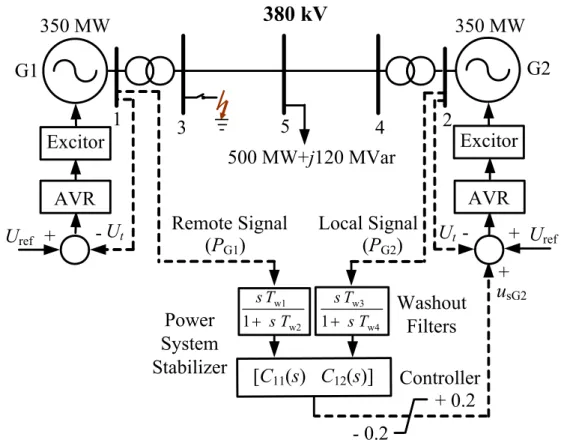
4.3.1 Power System Simulation Model ... 36
4.3.2 Design Results... 38
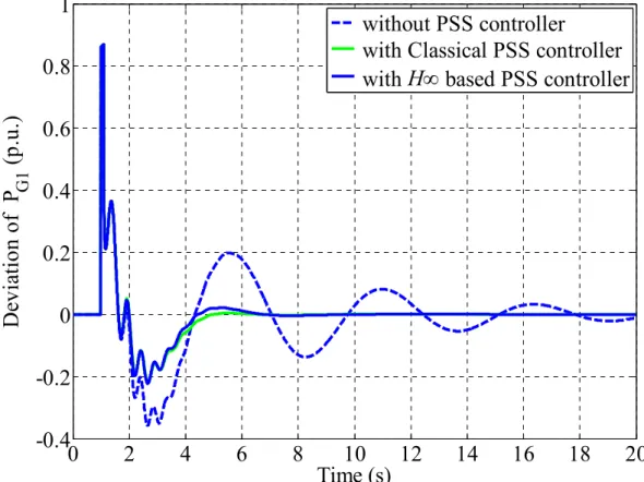
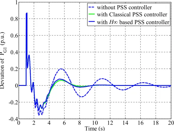
4.3.3 Time-Domain Simulation Results ... 40
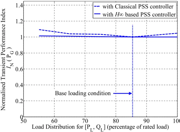
4.3.4 Robustness of Proposed Controller ... 42
Contents
5
Delayed-Input PSS... 455.1 Introduction ... 45
5.2 Time Delay in Power Systems... 46
5.2.1 Design of Delay Compensator ... 46
5.2.2 Pade Approximation Method for Constant Delay ... 48
5.2.3 LFT Method for Time Delay Uncertainty ... 50
5.3 Application Results... 54
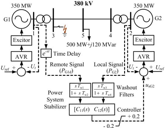
5.3.1 Power System Simulation Model ... 54
5.3.2 Design Results... 55
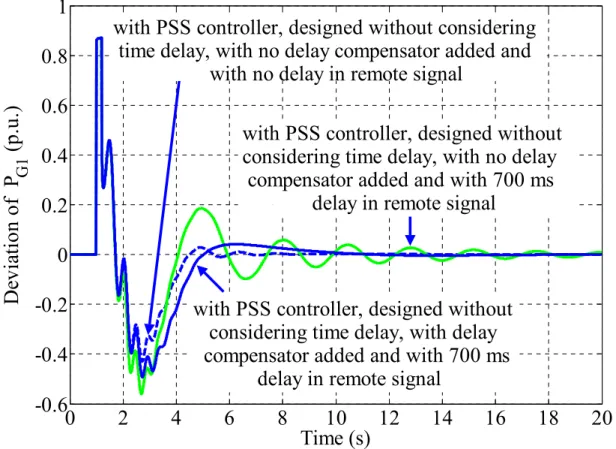
5.3.3 Time-Domain Simulation Results ... 59
5.4 Summary... 64
6
Mode Selective Damping of Power System Electromechanical Oscillations ... 676.1 Introduction ... 67
6.2 Concept of Mode Selective Damping... 68
6.3 Selection of Suitable Local and Remote Input Signals and Locations for PSS Controllers ... 69
6.3.1 Selection of Suitable Local and Remote Input Signals ... 69
6.3.2 Selection of Suitable Locations for PSS Controllers... 71
6.4 Design of Robust H∞-based PSS Controllers for Power Systems... 72
6.4.1 Problem Formulation... 72
6.4.2 Sequential Design of Controllers ... 73
6.5 Application Results... 74
6.5.1 Power System Simulation Model ... 74
6.5.2 Selection of Suitable Local and Remote Input Signals and Locations for PSS Controllers in the Test System ... 76
6.5.3 Design Results... 81
6.5.4 Time-Domain Simulation Results ... 90
6.6 Summary... 94
7
Mode Selective Damping of Electromechanical Oscillations for Very Large Power Systems... 977.1 Introduction ... 97
7.2 Lower-Order State-Space Model Identification... 98
7.3 Application Results... 99
7.3.1 Power System Simulation Model ... 99
7.3.2 Selection of Suitable Local and Remote Input Signals and Locations for PSS Controllers in the Test System ... 101
7.3.3 Design Results... 108
Contents
7.4 Summary... 117
8
Conclusions and Future Work... 1198.1 Conclusions ... 119
8.2 Future Work... 124
Appendices ... 127
Appendix A. Two-Machine Test System Data ... 127
Appendix B. Three-Machine, Three-Area Test System Data ... 129
References ... 133
Acronyms ... 139
Curriculum Vitae ... 141
Chapter 1
Introduction
1.1 Motivation
Recently, the number of bulk power exchanges over long distances has in-creased as a consequence of deregulation of the electrical energy markets worldwide and the extensions of large interconnected power systems. More-over, the power transfers have also become somewhat unpredictable as dic-tated by market price fluctuations. The integration of offshore wind generation plants into the existing network is also expected to have a significant impact on the power flow of system as well as the dynamic behavior of the network. The expansion of the transmission grids, on the other hand, is very little due to environmental and cost restrictions. The result is that the available transmis-sion and generation facilities are highly utilized with large amounts of power interchanges taking place through tie-lines and geographical regions. The tie lines operate near their maximum capacity, especially those connected to the heavy load areas. As a result, the system operation can find itself close to or outside the secure operating limits under severe contingencies. Stressed oper-ating conditions can increase the possibility of inter-area oscillations between different control areas and even breakup of the whole system [1].
Reliability and good performance are necessary in power system operation to ensure a safe and continuous energy supply with quality. However, weakly damped low frequency electromechanical oscillations (also called inter-area oscillations), inherent to large interconnected power systems during transient conditions, are not only dangerous for the reliability and performance of such
Chapter 1 Introduction
systems but also for the quality of the supplied energy. The power flows over certain network branches resulting from generator oscillations can take peak values that are dangerous from the point of view of secure system operation and lead to limitations in network control.
Inter-area oscillations may cause, in certain cases, operational limitations (due to the restrictions in the power transfers across the transmission lines) and/or interruption in the energy supply (due to loss of synchronism among the system generators). Also, the system operation may become difficult in the presence of these oscillations.
Even today, when voltage problems are by far, more important for network operators than damping control, large disturbances tend to induce wide-area low frequency oscillations in major grids throughout the world: at 0.6 Hz in the Hydro-Quebec system [2], [3], 0.2 Hz in the western North-American in-terconnection [4], [5], 0.15-0.25 Hz in Brazil [6] and 0.19-0.36 Hz in the UCTE/CENTREL interconnection in Europe [7]. The recent 2003 blackout in eastern Canada and US was equally accompanied by severe 0.4 Hz oscilla-tions in several post-contingency stages [8]. The two famous WECC cases in the summers of 1996 and 2000 were both associated with poorly damped in-ter-area oscillations under conditions of high power transfer on long paths [5].
With the heavier power transfers ahead, the damping of inter-area oscilla-tions will decrease unless new lines are built or other heavy and expensive high-voltage equipment such as series-compensation is added to the grid’s substations. The construction of new lines, however, is restricted by environ-mental and cost factors. Therefore, achievement of maximum available trans-fer capability as well as a high level of power quality and security has become a major concern. This concern requires the need for a better system control, leading to damping improvement.
1.1 Motivation
Most of the existing approaches for damping measures are initiated merely from the point of view of single subsystems, which are independent in their operation. The damping measures are not coordinated with other regions. In contrast to these measures of a local nature, the system as a whole should be considered.
It is found that if remote signals from one or more distant locations of the power system are applied to the controller design, the system dynamic per-formance can be enhanced for the inter-area oscillations [9]. The basic mechanism of damping remains as the production of damping torque in syn-chronous generators through the use of appropriate field excitation.
New distributed instrumentation technology using accurate phasor meas-urement units (PMUs) has developed in recent years to become a powerful source of wide-area dynamic information. The recent advances in wide area measurement system (WAMS) technologies using PMUs can deliver syn-chronous phasors and control signals at a high speed [2], [5]. PMUs are de-ployed at strategic locations on the grid and obtain a coherent picture of the entire network in real time [10]. PMUs measure positive sequence voltages and currents at different locations of the grid. Global Positioning System (GPS) technology ensures proper time synchronization among several global signals [10]. The measured global signals are then transmitted via modern telecommunication equipment to the controllers.
The signals from PMUs (PMUs located remote to the controllers) are re-ferred to as remote stabilizing signals. The remote signals are often rere-ferred to as global signals to illustrate the fact that they contain information about over-all network dynamics as opposed to local control signals which lack adequate observability of some of the significant inter-area modes [2]. For local modes, the largest residue is associated with a local signal, e.g., generator rotor speed
Chapter 1 Introduction
signal for PSS. But for inter-area modes, the local signals may not be the ones with maximum observability. The signal with maximum observability for a particular mode can be from a remote location or combined information from several locations.
Aboul-Ela and others [11] have proposed a two-level design of PSS and SVC controller using global signals. In [2], a decentralized/hierarchical struc-ture is proposed. Wide-area signals based PSS is used to provide additional damping.
Simulation studies have shown a high sensitivity of inter-area oscillations to generator voltage controller and hydro turbine governor settings [12]. Therefore, and because of the relatively low cost, measures to alleviate inter-area oscillations should be focused on power system controllers. The use of a supplementary control added to the Automatic Voltage Regulator (AVR) is a practical and economic way to supply additional damping to electromechani-cal oscillations. The first supplementary control for such task was proposed at the end of 1960’s [13], and is usually known as Power System Stabilizer (PSS). PSS units have long been regarded as an effective way to enhance the damping of electromechanical oscillations in power system [13]. The PSS provides supplementary control action through the excitation system of gen-erators and thus aids in damping the oscillations of synchronous machine ro-tors via modulation of the generator excitation. The supplemental damping is provided by an electric torque, applied to the rotor, which is in phase with the speed variation. The action of PSS, in this way, extends the angular stability limits of a power system.
For damping of local generator swings, PSSs have been established in the past [14], [1]. To enable damping of inter-area oscillations likewise with PSS, special control structures with additional signal inputs and well adapted
pa-1.1 Motivation
rameter tunings are necessary. Since the first proposal of PSS at the end of 1960’s, various control methods have been proposed for PSS design to im-prove overall system performance. Among the classical methods used are the phase-compensation method and the root-locus method. Among these, con-ventional PSS of the lead-lag compensation type [13], [15], [16] has been adopted by most utility companies because of its simple structure, flexibility and ease of implementation. Since power systems are highly nonlinear, con-ventional fixed-parameter PSSs cannot cope with changes in the operating conditions during normal operation and the system often tends to be unstable. Proper design of any control system that takes into account the continual changes in the structure of the network is, therefore, necessary to guarantee robustness over wide operating conditions in the system.
Robust control provides an effective approach to stabilize a power system over a wide range of operating conditions. Robust control approach deals with uncertainties introduced by variations of operating conditions and in this way, it guarantees system robustness to disturbances under various operating condi-tions. If the damping controller design is based on the robustness principle, minor errors in modeling will be alleviated and the closed-loop system will maintain satisfactory performance level.
Since last four decades, new PSS design methodologies based on robust control are proposed. Among many techniques available in the control litera-ture, H∞ has received considerable attention in the design of PSSs. The H∞
controller is characterized by the feature that the order of the controller is al-ways equal to the order of the generalized plant model, i.e., equal to the order of original plant plus the order of the weighting functions [17]. Higher order controllers may be too complex regarding practical implementation. Imple-mentation of higher order controllers will lead to high cost, difficulty in
com-Chapter 1 Introduction
missioning, poor reliability and potential problems in maintenance. Higher or-der controllers when implemented in real time configurations can create unde-sirable effects such as time delays. Therefore, lower order controllers having simpler designs are sought. In this study, balanced residualization technique [18] is used to reduce the order of controllers.
This research mainly focuses on the problem of improving the performance of conventional PSS, for a better damping of inter-area oscillations, by using instantaneous measurements from remote locations of the grid as its supple-mentary inputs.
1.2 Objectives
The concept presented in this study consists of the assumption that the PSS inputs are formed by measured variables coming from the whole system, i.e., particularly also from remote generators [19]. In this way, each PSS receives more complete measuring information about the inter-area oscillations to be damped. It is possible to use any of the variables from the generators, e.g., generator rotor speeds or angles or variables not assigned to generators, e.g. selected tie-line power flows as remote input signals to the controller. In gen-eral, the PSS controllers to be designed in this study are each of the multi-input, single-output (MISO) type. From the view point of power system engi-neering, the proposed PSS controller concept can be interpreted as a system of second level PSSs using additionally global measuring information. In this way design of PSS controllers is carried out for attaining a damping behavior which is in favor to the entire power system and not only to certain subsys-tems.
1.2 Objectives
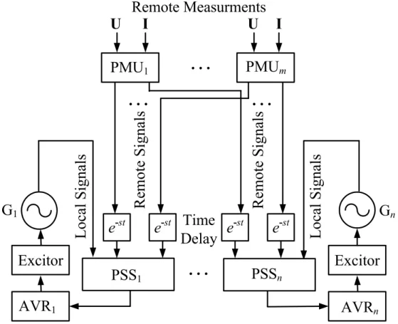
Figure 1.1 describes the basic architecture used in this work. It consists of a set of n PSSs located at specially selected generators G1,...,Gn together with m
PMUs which are remote to the PSSs. The PSSs are acting on the reference in-puts of the voltage regulators. In the context of wide-area stabilizing control of bulk power systems, the architecture shown in Figure 1.1 has higher opera-tional flexibility and reliability, especially when some remote signals are lost. Under such circumstances, the controlled power system is still viable (al-though with a reduced performance level), owing to the fact that a fully autonomous and decentralized layer without any communication link is al-ways present to maintain a standard performance level. As the global informa-tion is required only for some oscillatory modes, only a few PSS sites with the highest controllability of these modes need be involved in the supplementary global-signal-based actions. Remote Measurments . . . U I U I PMU1 PMUm . . . Time Delay . . . Local Signals Re mote Sign als PSS1 e-st e-st G1 AVR1 Excitor . . . Remote Signals PSSn Local Signals e-st e-st Gn AVRn Excitor
Chapter 1 Introduction
The main contribution of this thesis is to improve the performance of con-ventional PSS by using instantaneous measurements from remote locations of the grid. The research described herein will address the following objectives:
(i) The design of a local H∞-based PSS controller which uses wide-area
or global signals as additional measuring information from suitable remote network locations where the oscillations are well observable. (ii) In the proposed approach, remote signals, which are used as
supple-mentary inputs to the PSS controller, may arrive after a certain com-munication delay introduced by their transmission and processing in WAMS. Therefore, it is necessary to investigate the impact of time delay, in the remote input signal of the PSS controller, on the pro-posed approach. Also, the methods for dealing with the effects of time delay need to be investigated.
(iii) The design of local decentralized PSS controllers, using selected suit-able remote signals as supplementary inputs, for a separate better damping of specific inter-area modes. Each local PSS controller is de-signed separately for each of the inter-area modes of interest. The PSS controller uses only those local and remote input signals in which the assigned single inter-area mode is most observable and is located at a generator which is most effective in controlling that mode. The local PSS controller, designed for a particular single inter-area mode, also works mainly in a frequency band given by the natural frequency of the assigned mode.
(iv) The design of controllers is usually carried out on small systems. The power system, in practical, is large in size. The large-scale power sys-tems models, consisting of thousands of states, are impractical for
1.3 Outline
control design without extensive order reduction. The mode selective damping approach, described in (iii), is extended to realistic large-scale power systems by using system identification technique for de-riving lower order state-space models suitable for control design. The complete, large-scale multi-input, multi-output (MIMO) power sys-tem is used directly as the basis for building the required lower-order state-space or transfer function equivalent model. The lower-order model is identified by probing the network in open loop with low-energy pulses or random signals. The identification technique is then applied to signal responses, generated by time-domain simulations of the large-scale model, to obtain reduced-order model. Lower-order equivalent models, thus obtained, are used for the final selection of suitable local and remote input signals for PSS controllers, for the se-lection of suitable locations of PSS controllers and for the design of PSS controllers.
1.3 Outline
The subsequent chapters of this dissertation are organized as follows:
Chapter 2 provides a general description of the power system stability phe-nomena including fundamental concepts, classification, and definitions of as-sociated terms.
Chapter 3 presents the modeling and analysis of large power system dy-namics.
Chapter 4 describes the development of a robust H∞-based dynamic output
ap-Chapter 1 Introduction
proach used for the design of full order controller is also described in this chapter. The full order controller is then reduced to a first order one using model reduction techniques. The effectiveness of the designed PSS controller is demonstrated through digital simulation studies on a test power system.
Chapter 5 presents the impact of time delay, introduced by remote signal transmission and processing in WAMS, on the performance of an H∞-based
PSS controller, designed in chapter 4. Three methods for dealing with the ef-fects of time delay are presented. This chapter then describes the design of PSS controllers, using wide area or global signals as additional measuring in-formation, considering time delay in the remote signals. Digital simulation studies on a two-machine power system are conducted to investigate effec-tiveness of the proposed controller during system disturbances.
Chapter 6 deals with the design of local decentralized robust H∞-based PSS
controllers using remote signals as supplementary inputs, for a better damping of inter-area oscillations, in a manner that each decentralized PSS controller is designed separately for each of the inter-area modes of interest. The effective-ness of the resulting PSS controllers is demonstrated through digital simula-tion studies conducted on a test three-machine, three-area power system.
Chapter 7 presents the extension of the approach described in Chapter 6 to large-scale power systems. Application of system identification technique for deriving lower-order state-space models from large-scale models is also pre-sented in this chapter. The proposed approach is applied to a test sixteen-machine, three-area power system to show the effectiveness of the designed PSS controllers for a better damping of inter-area oscillations.
Chapter 8 summarizes the work presented in this dissertation. The main contributions of this dissertation are highlighted.
Chapter 2
Power System Stability
2.1 Introduction
Power system stability has been recognized as an important problem for se-cure system operation since the 1920s [20], [21]. Many major blackouts caused by power system instability have illustrated the importance of this phenomenon [22]. Historically, transient instability has been the dominant stability problem on most systems, and has been the focus of much of the in-dustry’s attention concerning system stability. As power systems have evolved through continuing growth in interconnections, use of new technolo-gies and controls, and the increased operation in highly stressed conditions, different forms of system instability have emerged. For the satisfactory design and operation of power systems, a clear understanding of different types of in-stability and relationship between them is necessary. Therefore, there is a need for the proper definition and classification of power system stability.
2.2 Definition and Classification of Power System
Stability
Power system stability is the ability of an electric power system, for a given initial operating condition, to either regain a new state of operating equilib-rium or return to the original operating condition (if no topological changes occurred in the system) after being subjected to a physical disturbance, with
Chapter 2 Power System Stability
most system variables bounded so that practically the entire system remains intact [23].
The power system is a highly nonlinear system that operates in a constantly changing environment. The loads, generator outputs and main operating pa-rameters change continually. Power systems are subjected to a wide range of small and large disturbances. Small disturbances in the form of incremental changes in the system load or generation occur continually. Large distur-bances are the disturbances of a severe nature, such as a short circuit on a transmission line or loss of a large generator. A large disturbance may lead to structural changes due to the isolation of the faulted elements. When subjected to a disturbance, the stability of the system depends on the initial operating condition as well as the nature of the disturbance.
Power system stability can be classified into different categories and sub-categories as shown in Figure 2.1 [23], [1]. The descriptions of the corre-sponding forms of stability phenomena are given in the following sub-sections. Non-Oscillatory Stability Oscillatory Stability Rotor Angle Stability Frequency
Stability StabilityVoltage Small-Distrubance Angle Stability Large-Distrubance Voltage Stability Small-Distrubance Voltage Stability Large-Distrubance Angle Stability or Transient Stability Power System Stability
2.2 Definition and Classification of Power System Stability
2.2.1 Rotor Angle Stability
Rotor angle stability refers to the ability of synchronous machines of an inter-connected power system to remain in synchronism after being subjected to a disturbance. It depends on the ability to maintain/restore equilibrium between electromagnetic torque (generator output) and mechanical torque (generator input) of each synchronous machine in the system. Instability that may result occurs in the form of increasing angular swings of some generators leading to their loss of synchronism with other generators.
The change in electromagnetic torque (ΔTe) of a synchronous machine fol-lowing a perturbation can be resolved into two components: (i) Synchronizing torque component, in phase with rotor angle deviation (Δδ), and (ii) Damping torque component, in phase with the speed deviation (Δω). Mathematically, this can be expressed as follows:
ω δ Δ Δ
ΔTe =Ts +TD (2.1)
where
TsΔδ is the synchronizing torque component of torque change. Ts is the synchronizing torque coefficient.
TDΔω is the damping torque component of torque change. TD is the damp-ing torque coefficient.
System stability depends on the existence of both components of torque for each of the synchronous machines. Lack of sufficient synchronizing torque causes an increase in rotor angle through a nonoscillatory or aperiodic mode. This form of instability is known as aperiodic or nonoscillatory instability. Lack of damping torque causes rotor oscillations of increasing amplitude. This form of instability is known as oscillatoryinstability.
Chapter 2 Power System Stability
• Small-disturbance (or small-signal) rotor angle stability • Large-disturbance rotor angle stability or transient stability
2.2.1.1 Small-Disturbance Rotor Angle Stability
Small-disturbance (or small-signal) rotor angle stability is concerned with the ability of the power system to maintain synchronism under small disturbances. The disturbances are considered to be sufficiently small that linearization of system equations is permissible for purposes of analysis [1], [24], [25] and the use of powerful analytical tools of linear systems is allowed to aid in the analysis of stability characteristics and in the design of corrective controls [24]. The results of the system response to small disturbances are usually given in terms of eigenvalues and eigenvectors.
In today’s power systems, small-disturbance rotor angle stability problem is usually associated with insufficient damping of oscillations [23]. Small-disturbance rotor angle stability problems may be either local or global in na-ture. The descriptions of these problems are given below:
• Local problems involve a small part of the power system, and are usually associated with rotor angle oscillations (swinging) of a single power plant (units at a generating station) against the rest of the power system. Such oscillations are called local plant mode oscilla-tions. The term local is used because the oscillations are localized at one station or a small part of the power system. Stability (damping) of these oscillations depends on the strength of the transmission sys-tem as seen by the power plant, generator excitation control syssys-tems and plant output [1]. When a generator is tied to a power system via a long radial line, it is susceptible to local mode oscillations [26].
2.2 Definition and Classification of Power System Stability
• Global problems are caused by interactions among large groups of generators. They are associated with rotor angle oscillations (swing-ing) of a group of generators in one area of an interconnected power system against a group of generators in another area. Such oscilla-tions are called inter-area mode oscillations.
The time frame of interest in small-disturbance stability studies is on the order of 10 to 20 seconds following a disturbance [23].
2.2.1.2 Large-Disturbance Rotor Angle Stability or Transient Stability
Large-disturbance rotor angle stability or transient stability is concerned with the ability of the power system to maintain synchronism when subjected to a severe disturbance, such as a short circuit on a transmission line. The resulting system response involves large excursions of generator rotor angles and is in-fluenced by the nonlinear power-angle relationship.
Transient stability depends on both the initial operating state of the system and the severity of the disturbance. Usually, the system is altered so that the post-disturbance steady-state operation differs from that prior to the distur-bance. Instability is usually in the form of aperiodic angular separation due to insufficient synchronizing torque, manifesting as first swing instability [23]. However, in large power systems, transient instability may not always occur as first swing instability associated with a single mode; it could be a result of superposition of a slow inter-area swing mode and a local-plant swing mode causing a large excursion of rotor angle beyond the first swing [1].
The time frame of interest in transient stability studies is usually 3 to 5 sec-onds following the disturbance. It may extend to 10–20 secsec-onds for very large systems with dominant inter-area swings [23].
Chapter 2 Power System Stability
Small-disturbance rotor angle stability as well as transient stability is cate-gorized as short term phenomena.
2.2.2 Voltage Stability
Voltage stability refers to the ability of a power system to maintain steady voltages at all buses in the system after being subjected to a disturbance from a given initial operating condition. It depends on the ability to main-tain/restore equilibrium between load demand and load supply from the power system. Instability that may result occurs in the form of a progressive fall or rise of voltages of some buses. However, the most common form of voltage instability is the progressive drop in bus voltages. A possible outcome of volt-age instability is loss of load in an area, or tripping of transmission lines and other elements by their protective systems leading to cascading outages. Loss of synchronism of some generators may result from these outages or from op-erating conditions that violate field current limit [27].
As in the case of rotor angle stability, voltage stability can also be classi-fied into the following subcategories:
• Small-disturbance voltage stability refers to the system’s ability to maintain steady voltages when subjected to small perturbations such as incremental changes in system load.
• Large-disturbance voltage stability refers to the system’s ability to maintain steady voltages following large disturbances such as system faults, loss of generation, or circuit contingencies. The study period of interest may extend from a few seconds to tens of minutes.
2.2 Definition and Classification of Power System Stability
As the time frame of interest for voltage stability problems may vary from a few seconds to tens of minutes, therefore, voltage stability may be either a short-term or a long-term phenomenon.
2.2.3 Frequency Stability
Frequency stability refers to the ability of a power system to maintain steady frequency within a nominal range following a severe system upset resulting in a significant imbalance between generation and load [23]. It depends on the ability to maintain/restore equilibrium between system generation and load, with minimum unintentional loss of load. Instability that may result occurs in the form of sustained frequency swings leading to tripping of generating units and/or loads.
Generally, frequency stability problems are associated with inadequacies in equipment responses, poor coordination of control and protection equipment, or insufficient generation reserve [28]- [31].
During frequency excursions, the characteristic times of the processes and devices that are activated will range from fraction of seconds, corresponding to the response of devices such as under-frequency load shedding and genera-tor controls and protections, to several minutes, corresponding to the response of devices such as prime mover energy supply systems and load voltage regu-lators. Therefore, frequency stability may be a short-term phenomenon or a
Chapter 2 Power System Stability
2.3 Small Signal Stability Assessment of Power
Systems using Modal Analysis
A power system typically comprises a large number of components. Besides, the behavior of most of these components is described through differential-algebraic equations. Hence, in general, the dynamic behavior of a power sys-tem can be described by a set of n first order nonlinear ordinary differential equations, denominated as state equations, together with a set of algebraic equations, developed on the basis of the system model. Using vector-matrix notation, the set of differential-algebraic equations can be expressed as fol-lows [1]: ) , (x u f x& = (2.2) ) , (x u g y = (2.3) where
x=
[
x1 x2 L xn]
T is the vector of state variables, referred to as state vector,[
]
T 2 1 u ur u L =u is the vector of input signals to the system, re-ferred to as input vector,
[
]
T2
1 y ym
y L
=
y is the vector of system output variables, re-ferred to as output vector,
[
]
T2
1 f fn
f L
=
f is the vector of nonlinear functions defining state variables in terms of state and input vari-ables,
[
]
T 2 1 g gm g L =g is the vector of nonlinear functions defining state variables in terms of state and input vari-ables,
2.3 Small Signal Stability Assessment of Power Systems using Modal Analysis
where n is the order of the system, r is the number of inputs and m is the num-ber of outputs. The input signals to the system (ui) are the external signals that
influence the performance of the system.
From the classification of power system stability, described in Section 2.2, the small signal stability is focused on small disturbances. Thus, to analyze the small signal stability of the system mathematically, the disturbances can be considered to be small in magnitude in order to linearize the equations that describe the dynamics of the system.
For small perturbation of the system from its initial operating point (the point around which small signal performance is to be investigated), (2.2) and (2.3) can be expressed in linearized form as follows [1]:
) ( Δ ) ( Δ ) ( Δx& t = A x t +B u t (2.4) ) ( Δ ) ( Δ ) ( Δy t = C x t +D u t (2.5) where
Δ is the prefix which denotes a small deviation,
A is the state or plant matrix of size n×n,
B is the control or input matrix of size n×r,
C is the output matrix of size m×n,
D is the (feed-forward) matrix which defines the proportion of input which appears directly in the output, size m×r
The eigenvalues of the state matrix A determine the time domain response of the system to small perturbations and therefore provide valuable informa-tion regarding the stability characteristics of the system. The stability of the system is determined by the eigenvalues as follows:
Chapter 2 Power System Stability
(i) A real eigenvalue corresponds to a non-oscillatory mode. A negative real eigenvalue represents a decaying mode. A positive real eigen-value represents aperiodic instability.
(ii) Complex eigenvalues occur in conjugate pairs, and each pair corre-sponds to an oscillatory mode. If all eigenvalues have a negative real part then all oscillatory modes decay with time and the system is said to be stable [24]. The critical eigenvalues are characterized by being complex (also denominated swing modes or oscillatory modes) and located near the imaginary axis of the complex plane [32]. For a com-plex pair of eigenvalues
λ
=σ
± jω
, the real component of the ei-genvalues (σ) gives the damping, and the imaginary component (ω) gives the frequency of oscillation. A negative value of σ represents a damped oscillation whereas a positive value of σ represents oscillation of increasing amplitude. The frequency of oscillation in Hz is given by f =ω
2π
. The damping ratio (ζ) is given by:2 2
ω
σ
σ
ζ
+ − = (2.6)For any eigenvalue λ, there are the corresponding vectors: right eigenvec-tor, left eigenvector and the participation vector. The associated right eigen-vector gives the mode shape, i.e., the relative activity of the state variables when a particular mode is excited [1]. The magnitudes of the elements of right eigenvector give the extents of the activities of the n state variables in the ith -mode, and the angles of the elements give phase displacements of the state variables with regard to the mode [1]. The associated left eigenvector is refer-ring to the initial conditions, since it has a direct effect on the amplitude of a mode excited by a specific input [24].
2.4 Summary
The participation vector combines the right and left eigenvectors. The ele-ment pki of the participation vector termed as the participation factor [33], is a
measure of the relative participation of the kth state variable in the ith-mode, and vice versa. The participation factor pki measure the sensitivity of the ith
-eigenvalue to a change in the kth diagonal element of the state matrix (akk),
mathematically, kk i ki a pf =∂
λ
∂ (2.7)2.4 Summary
This chapter is focused on the issue of stability definition and classification in power systems from a fundamental as well as practical point of view. A pre-cise definition of power system stability that is taking into consideration all forms is provided. The main focus of the chapter is to provide a systematic classification of power system stability, and the identification of different categories of stability behaviors that are important in power system stability analysis. The chapter also provides description of small signal stability as-sessment using modal analysis.
Chapter 3
Power System Modelling
3.1 Introduction
This chapter briefly reviews the issue of power system modeling that is useful for analysis and control design in later chapters. Power System Dynamics (PSD) software [34], used in this dissertation for simulation studies, is dis-cussed in terms of sets of structural and functional subdivisions. These subdi-visions precisely reveal the interrelations/interactions among the individual components as well as the computational structure for describing real large power systems. Further, the linearized dynamic model is decomposed as in-terconnected subsystems that could be used to design decentralized controllers for power system. Moreover, the problem of model reduction for large power systems is discussed by deriving a relatively low-order model which is neces-sary for applying controller design techniques.
3.2 Nonlinear Modelling and Simulation of Power
Systems
Modern power systems are characterized by complex dynamic behaviors ow-ing to their size and complexity. Power systems, even in their simplest form, exhibit nonlinear and time-varying behaviors. Moreover, there are numerous equipment found in today’s power systems, namely: (i) synchronous genera-tors; (ii) loads; (iii) reactive-power control devices like capacitor banks and shunt reactors; (iv) power electronically switched devices such as static Var
Chapter 3 Power System Modelling
Compensators (SVCs), and currently developed flexible AC transmission sys-tems (FACTS) devices; (v) series capacitors and other equipments. Precise modeling of these equipments plays important role for analysis and simulation studies of the whole system.
In order to obtain an appropriate model of power systems, each equipment or component of the power system should be described by appropriate alge-braic and/or differential equations. Dynamic model of power systems is then obtained by combining the dynamic models of these individual components together with the associated algebraic constraints. In general, the dynamic model of power systems can be formulated by the nonlinear differential-algebraic equations given as follows:
) , , , ( ) ( f x y u p x& t = (3.1) ) , , , ( 0=g x y u p (3.2)
where x(t), y(t) and u(t) are the state‚ output and input variables of the power system, respectively. p(t) represent parameters and/or effects of control at par-ticular time in the system.
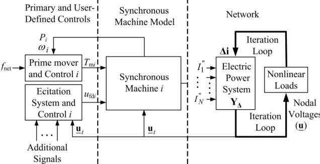
Modeling of power system is further discussed based on the PSD software that is used in this dissertation for power flow analysis, linearization of nonlinear differential-algebraic equations, calculation of eigenvalues and ei-genvectors and nonlinear time-domain simulation of power systems. Figure 3.1 shows the main structural components and their interrelations that are functionally implemented in the PSD software environment. A brief explana-tion of the PSD is given as follows:
3.2 Nonlinear Modelling and Simulation of Power Systems Synchronous Machine Model Synchronous Machine i
Primary and User- Defined Controls '' 1 I '' N I Electric Power System . . . . . . Nonlinear Loads Iteration Loop Nodal Voltages Network i ωPi Tmi ufdi
fnet Prime mover
and Control i . . . Additional Signals Ecitation System and Control i Iteration Loop Δ Y Δi t u t u (u)
Figure 3.1Integration of synchronous machine model into complete power system model
• The block in the middle of Figure 3.1 is used to describe the dynam-ics of synchronous machines. Synchronous machines have major in-fluence on the overall dynamic performance of power systems due to their characteristics. A reduced 5th-order model, where stator tran-sients (i.e., stator flux linkage derivatives dψd dt, dψq dt ) are ne-glected [35], is used for all synchronous machines in this study. The model consists of a set of differential and a set of algebraic equations. Input variables to the models are the complex terminal voltage
u
ti, the field excitation voltage ufdi, and the mechanical turbine torqueTmi. Moreover, the injected currents into the network, which depend
on the corresponding state variables of the synchronous machines, are used as input to the algebraic network equations.
• The nodal voltages shown at the bottom of the right-side are com-puted by solving the algebraic network equations of the nodal admit-tance matrix. Nonlinear voltage dependent loads are incorporated in
Chapter 3 Power System Modelling
the system where the solutions for updating injection currents are car-ried out iteratively.
• The blocks in the left of Figure 3.1 represent the voltage and gover-nor controllers. The govergover-nor control block contains, in addition to the direct primary control of turbine torque (i.e., the governor mecha-nism), the mechanical dynamics of the equipment, such as the turbine or boiler that tie to the system dynamically through the governor con-trol valve. Similarly, the voltage concon-trol block typically includes voltage regulators and exciters. Moreover, user-defined controller structures can be easily incorporated either through voltage or gover-nor controller sides and such options give greater flexibility in analy-sis and simulation studies.
3.3 Modelling of Power Systems for Small-Signal
Analysis
The starting model for small-signal analysis in power system is derived by linearizing the general nonlinear dynamic model of (3.1) and (3.2) around an operating (or equilibrium) point (x0, y0, u0, p0) and is given as follows:
) ( Δ ) ( Δ ) ( Δ ) ( Δx& t =A x t +B1 u t +B2 p t (3.3) where Δx(t)=x(t)−x0, Δu(t)=u(t)−u0,and Δp(t)=p(t)−p0 . x(t), y(t),
u(t) and p(t) are the actual values of states, outputs, inputs and parameters re-spectively. Note that in considering the linear systems of the form (3.3), the symbol “Δ” will be omitted in the remaining part of this thesis.
Depending on how detailed the model in (3.1) and (3.2) is used, the result-ing linearized model (3.3) may or may not be applicable to study particular
3.4 Summary
physical phenomena in power system. Any disturbance, acting on the system, affects all system states, and their exact changes are complex and can only be analyzed by using the full-order model. Despite this fact, in order to avoid un-necessary complexity, much effort has been devoted to the reduction of power system dynamic models. Moreover, model-reduction techniques have also an-other importance in power systems. In a large power system consisting of weakly connected subsystems, it is possible to derive a relatively low-order model relevant for understanding the interactions among the subsystems (in-ter-area dynamics), as well as detailed models relevant for understanding the dynamics inside each subsystem (intra-area dynamics) [34], [36]- [38]. The small-signal stability analysis of these developed models is then carried out. Basic analysis uses the elementary result that, given u(t) = 0 and p(t) = 0, the system of time-invariant linear differential equations (3.3) will have a stable response to initial conditions x(0) = 0 when all eigenvalues of system matrix
A are in the left-half plane. Moreover, the robustness of the system dynamics can be analyzed using the more involved sensitivity techniques with respect to parameter uncertainties [34], [36].
3.4 Summary
In this chapter, modeling and analysis of large power system dynamics are discussed. The chapter briefly discussed real large power systems representa-tion with respect to the PSD software where the latter is used for analysis and simulation studies in this dissertation. Moreover, the model for the small-signal analysis in power system is also presented in this chapter.
Chapter 4
Robust PSS Controller Design using
Supple-mentary Remote Signals
4.1 Introduction
This chapter presents the design of a local H∞-based PSS controller which
uses wide-area or global signals as additional measuring information from suitable remote network locations where the oscillations are well observable. The controller, placed at suitably selected generators, provide control signals to the AVRs to damp out inter-area oscillations through the machines’ excita-tion systems. Electrical power outputs of generators have been used as input signals to the controller. To provide robust behavior, H∞ control theory
to-gether with an algebraic Riccati equation (ARE) approach has been applied to design the proposed controller. Digital simulation studies are conducted on a test power system to investigate the effectiveness of the proposed controllers during system disturbances.
4.2 Robust
H
∞Output Feedback Controller Design
for Power Systems
4.2.1 Problem Formulation
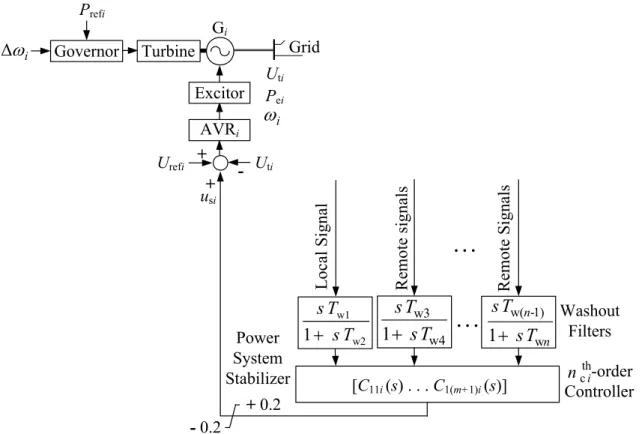
The general structure of the ith-generator together with the PSS block in a multi-machine power system is shown in Figure 4.1. Local and remote input signals of washout filters are assumed to be electrical power outputs of gen-erators. The outputs of washout filters are the inputs of the ith-controller. The
Chapter 4 Robust PSS Controller Design using Supplementary Remote Signals
washout filter prevents the controller from acting on the system during steady state. Power System Stabilizer + + - Urefi Uti usi i ω AVRi [C11i (s) . . . C1(m+1)i (s)] - 0.2 + 0.2 w2 w1 1 sT T s + w4 w3 1 sT T s + . . . Local Signal . . . Re mot e si gnal s Pei Excitor Uti Gi Grid Prefi i ω Δ Governor Turbine n n T s T s w 1) -w( 1+ Washout Filters Rem ote S ignals th ci n -order Controller
Figure 4.1 General structure of the ith-generator together with the PSS in a multi-machine power system
After augmenting the washout stage in the system, the ith-subsystem of the linear, time-invariant, continuous-time composite system which is composed of N subsystems, within the framework of H∞ design, is described by the
fol-lowing state-space model [39], [40]:
) ( ) ( ) ( ) ( ) ( 1 2 , 1 t t t t t i i i i N i j j ij j i ii i A x A x B w B u x = + ∑ + + ≠ = & (4.1) ) ( ) ( ) ( ) (t 1i i t 11i i t 12i i t i C x D w D u z = + + (4.2) ) ( ) ( ) ( ) (t 2i i t 21i i t 22i i t i C x D w D u y = + + , i =1,…, N (4.3) where ni i(t)∈R
4.2 Robust H∞ Output Feedback Controller Design for Power Systems
mi
i(t)∈R
u is the vector of control input signals, pi
i(t)∈R
y is the vector of measured output signals available to the controller,
qi
i(t)∈R
z is the vector of exogenous regulated output signals including all regulated or controlled signals and tracking errors,
ir
i(t)∈R
w is the vector of exogenous input signals including noises, disturbances and reference or command signals for the
ith-subsystem, and
Aii, Aij, B1i, B2i, C1i, C2i, D11i, D12i, D21i and D22i are all constant
matri-ces with appropriate dimensions.
Moreover, it is assumed that there is no unstable fixed mode [41] with respect to C2 =diag
{
C21,C22,L,C2N}
, [Aij]N×Nand B2 =diag{
B21,B22,L,B2N}
.The complete system can be equivalently described by the following compos-ite equations: ) ( ) ( ) ( ) (t Ax t B1w t B2u t x& = + + (4.4) ) ( ) ( ) ( ) (t C1x t D11w t D12u t z = + + (4.5) ) ( ) ( ) ( ) (t C2x t D21w t D22u t y = + + (4.6) where,
[
T T]
T 2 T 1( ) ( ) ( ) ) (t x t x t xN t x = L , u(t) =[
u1T(t) u2T(t) L uTN(t)]
T,[
T]
T r T T 2 T 1 ( ) ( ) ( ) ( ) ) (t y t y t yN t y t y = L ,[
T]
T r T T 2 T 1( ) ( ) ( ) ( ) ) (t z t z t zN t z t z = L ,[
T T]
T 2 T 1 ( ) ( ) ( ) ) (t w t w t wN t w = L ,Chapter 4 Robust PSS Controller Design using Supplementary Remote Signals
[ ]
⎥ ⎥ ⎥ ⎦ ⎤ ⎢ ⎢ ⎢ ⎣ ⎡ = = × NN N N N N ij A A A A A A L M O M L 1 1 11 , B1 =diag{
B11,B12,L,B1N}
,{
21 22 2N}
2 diagB ,B , ,B B = L , C1 =diag{
C11,C12,L,C1N}
,{
21 22 2N}
2 diag C ,C , ,C C = L , D11 =diag{
D111,D112,L,D11N}
,{
121 122 12N}
12 diag D ,D , ,D D = L , D21 =diag{
D211,D212,L,D21N}
whereyr(t) is the vector of measured remote output signals available to the controller,
zr(t) is the vector of exogenous regulated remote output signals The following assumptions are imposed on the plant parameters:
(i) (A, B2) is stabilizable and (A, C2) is detectable; (ii) D12 and D21 have full rank;
(iii) ⎥ ⎦ ⎤ ⎢ ⎣ ⎡ − 12 1 2 D C B A jωI
has full column rank and ⎥
⎦ ⎤ ⎢ ⎣ ⎡ − 21 2 1 D C B A jωI has full row rank for all ω
(iv) D11 = 0q×r and D22 = 0p×m;
The dynamic output feedback controller considered for the system of (4.1)-(4.3) is given by: ) ( ) ( ) ( c c c r ci t A ix i t B iyi t x& = + (4.7) ) ( ) ( ) (t ci ci t ci ir t i C x D y u = + (4.8) where n i i(t) R c c ∈
x is the state vector of the ith-local independent controller,
nci is a specified dimension,
[
]
T T r T r(t) i (t) (t) i y y y = and4.2 Robust H∞ Output Feedback Controller Design for Power Systems
Aci, Bci, Cci, Dci, i =1, 2,…, N are constant matrices to be determined during
the design.
In this study, the design procedure deals with nonzero Dci, however, it can be
set equal to zero, i.e., Dci = 0, so that the ith-local independent controller is
strictly proper controller.
After augmenting the controller of (4.7) and (4.8) in the system of (4.1)-(4.3), the state space equation of ith-extended subsystem will have the follow-ing form: ∑ ≠ = + + + + = N i j j ij j i i i i i i i i i ii i t t t t , 1 2 2 1 2 2 ~ ( ) ~ ) ( ) ~ ~ ~ ( ) ( ~ ) ~ ~ ~ ( ) ( ~x. A B K C x B B K C w A x (4.9) ) ( ) ~ ~ ~ ( ) ( ~ ) ~ ~ ~ ( ) (t 1i 12i i 2i i t 11i 12i i 21i i t i C D K C x D D K D w z = + + + (4.10) where
[
T]
T c T( ) ( ) ) ( ~ t t t i i i x xx = is the augmented state vector for the ith-subsystem and ⎥ ⎥ ⎦ ⎤ ⎢ ⎢ ⎣ ⎡ = × × × ci ci i ci ci i n n n n n n ij ij 0 0 0 A A~ , ⎥ ⎥ ⎦ ⎤ ⎢ ⎢ ⎣ ⎡ = ×i i r n i i 0 B B~1 1 , ⎥ ⎥ ⎦ ⎤ ⎢ ⎢ ⎣ ⎡ = × × i m ci ci ci i n n n i n n i I 0 B 0 B~2 2 ,
[
i pi nci]
i = C 0 × C~1 1 , ⎥ ⎥ ⎦ ⎤ ⎢ ⎢ ⎣ ⎡ = × × × ci i ci ci i ci n q i n n n n i C 0 I 0 C 2 2 ~ , i i 11 11 ~ D D = ,[
p n i]
i i ci 12 12 ~ D 0 D = × , ⎥ ⎦ ⎤ ⎢ ⎣ ⎡ = × i r n i ci i 21 21 ~ D 0 D , ⎥ ⎦ ⎤ ⎢ ⎣ ⎡ = i i i i i c c c c D C B A KMoreover, the overall extended system can be equivalently described by the following composite equations:
) ( ) ~ ~ ~ ( ) ( ~ ) ~ ~ ~ ( ) ( ~ 2 D 2 1 2 D 2 t t t A B K C x B B K C w x. = + + + (4.11) ) ( ) ~ ~ ~ ( ) ( ~ ) ~ ~ ~ ( ) (t C1 D12KDC2 x t D11 D12KDD21 w t z = + + + (4.12) where
Chapter 4 Robust PSS Controller Design using Supplementary Remote Signals
[ ]
ij N×N = A A~ ~ , B~1 =diag{
B~11,B~12,L,B~1N}
,{
21 22 2N}
2 ~ , , ~ , ~ diag ~ B B B B = L , C~1 =diag{
C~11,C~12,L,C~1N}
,{
21 22 2N}
2 ~ , , ~ , ~ diag ~ C C C C = L , D~11 =diag{
D~111,D~112,L,D~11N}
,{
121 122 12N}
12 ~ , , ~ , ~ diag ~ D D D D = L , D~21 =diag{
D~211,D~212,L,D~21N}
,{
K K KN}
KD =diag 1, 2,L,The overall extended system of (4.11) and (4.12) can be rewritten in a com-pact form as follows:
) ( ) ( ~ ) ( ~ cl cl t t t A x B w x. = + (4.13) ) ( ) ( ~ ) (t Cclx t Dclw t z = + (4.14) where Acl =A~ +B~2KDC~2, Bcl =B~1+B~2KDC~2 , Ccl =C~1 +D~12KDC~2, Dcl =D~11+D~12KDD~21
4.2.2 H
∞Controller Design using Riccati-based Approach
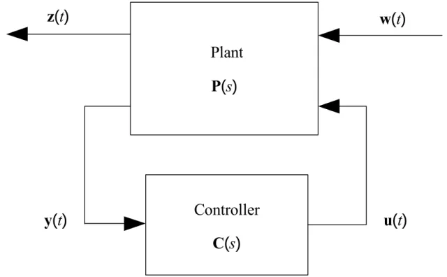
Any general system interconnection can be put in the general linear fractional transformation (LFT) framework shown in Figure 4.2, where P(s) is the gen-eralized plant or interconnected system, C(s) is the controller.
4.2 Robust H∞ Output Feedback Controller Design for Power Systems
P
(
s
)
C
(
s
)
Plant
Controller
w
(
t
)
u
(
t
)
z
(
t
)
y
(
t
)
Figure 4.2 General LFT frame work representing general interconnected system
Designing an H∞ output feedback controller for the system is equivalent to
that of finding the matrix KD, in (4.13) and (4.14), that satisfies an H∞ norm
bound condition on the closed loop transfer function
cl cl 1 cl cl( ) ) ( C A B D
Tzw s = sI − − + from disturbance w(t) to the controlled outputs z(t) in Figure 4.2, i.e., Tzw(s) ∞ <γ (for a given scalar constant
0 >
γ ). Moreover, transfer functionsTzw(s)must be stable [42]. An ARE ap-proach [43] can be applied to establish the existence of control strategy of (4.7) and (4.8) that internally stabilizes the closed loop transfer func-tionTzw(s)and satisfies a certain prescribed disturbance attenuation (or gain) level γ >0 on Tzw(s), i.e., Tzw(s) ∞ <γ . The matrices of dynamic output feedback control law of (4.7) and (4.8) are given by [43]: