Fast prediction of transonic aeroelasticity using computational fluid dynamics

(1)

Glasgow Theses Service http://theses.gla.ac.uk/

theses@gla.ac.uk

Woodgate, Mark A. (2008)

Fast prediction of transonic aeroelasticity

using computational fluid dynamics.

PhD thesis.

http://theses.gla.ac.uk/923/

Copyright and moral rights for this thesis are retained by the author

A copy can be downloaded for personal non-commercial research or

study, without prior permission or charge

This thesis cannot be reproduced or quoted extensively from without first

obtaining permission in writing from the Author

The content must not be changed in any way or sold commercially in any

format or medium without the formal permission of the Author

When referring to this work, full bibliographic details including the

author, title, awarding institution and date of the thesis must be given

(2)

Using Computational Fluid Dynamics

by

Mark Woodgate BSc.

A thesis submitted in partial fulfillment of the requirements for the degree of Doctor of Philosophy

University of Glasgow

Department of Aerospace Engineering September 2008

(3)

Declaration

I hereby declare that this dissertation is a record of work carried out in the Department of Aerospace Engineering at the University of Glasgow during the pe-riod from October 1999 to September 2008. The dissertation is original in content except where otherwise indicated.

September 2008

... (Mark Andrew Woodgate)

(4)

Abstract

The exploitation of computational fluid dynamics for non linear aeroelastic simulations is mainly based on time domain simulations of the Euler and Navier-Stokes equations coupled with structural models. Current industrial practice relies heavily on linear methods which can lead to conservative design and flight envelope restrictions. The significant aeroelastic effects caused by nonlinear aerodynamics include the transonic flutter dip and limit cycle oscillations. An intensive research effort is underway to account for aerodynamic nonlinearity at a practical computa-tional cost. To achieve this a large reduction in the numbers of degrees of freedoms is required and leads to the construction of reduced order models which provide compared with CFD simulations an accurate description of the dynamical system at much lower cost.

In this thesis we consider limit cycle oscillations as local bifurcations of equi-libria which are associated with degenerate behaviour of a system of linearised aeroelastic equations. This extra information can be used to formulate a method for the augmented solve of the onset point of instability - the flutter point. This method contains all the fidelity of the original aeroelastic equations at much lower cost as the stability calculation has been reduced from multiple unsteady computations to a single steady state one. Once the flutter point has been found, the centre mani-fold theory is used to reduce the full order system to two degrees of freedom. The thesis describes three methods for finding stability boundaries, the calculation of a reduced order models for damping and for limit cycle oscillations predictions. Re-sults are shown for aerofoils, and the AGARD, Goland, and a supercritical transport wing.

It is shown that the methods presented allow results comparable to the full order system predictions to be obtained with CPU time reductions of between one and three orders of magnitude.

(5)

Acknowledgements

I am grateful to BAE SYSTEMS, Engineering and Physical Sciences Re-search Council, MoD and DERA for funding this work as part of the programme of the Partnership for Unsteady Methods in Aerodynamics (PUMA) Defence and Aerospace Research Partnership (DARP).

I would like to thank my supervisor Professor Ken Badcock for this support, encouragement, guidance and patience over the past 8 years.

I would also like to thank all the members of the CFD Lab, past and present, for creating a stimulating working environment which is has been a privilege to work at over the years. I especially like to thank Professor Bryan Richards for this support during my early years at Glasgow University and Dr George Barakos for motivating me to get this work written up.

I am grateful to Professor Michael Henshaw and all the aerodynamicists at BAE SYSTEM Brough that made my years secondment there so productive and opened my eyes between practises used in the worlds of academia and business in the field of aeroelastics.

(6)

List of Most Relevant Publications

M.A. Woodgate and K.J. Badcock. Fast prediction of transonic aeroelastic

stability and limit cycles. AIAA Journal, vol 45(6):1370-1381, 2007.

M.A. Woodgate and K.J Badcock. A reduced order model for damping derived

from CFD based aeroelastic simulations. In 47th AIAA/ASME/ASCE/AHS/ASC

Structures, Structural Dynamics, and Materials Conference, Newport, Rhode

Island, 1-4 May 2006. AIAA-2006-2021.

K.J. Badcock and M.A. Woodgate. Aeroelastic damping model derived from discrete Euler equations. AIAA Journal, vol 44(11):2601-2611, 2006.

M.A. Woodgate, K.J. Badcock, A.M. Rampurawala, B.E. Richards, D. Nardini, and M.J. Henshaw. Aeroelastic calculations for the Hawk aircraft using the Euler equations. Journal of Aircraft, vol 42(4):1005-1012, 2005.

K.J. Badcock, M.A. Woodgate, and B.E. Richards. Direct aeroelastic bifurcation analysis of a symmetric wing based on the Euler equations. Journal of Aircraft, vol 42(3):731-737, 2005.

K.J. Badcock, M.A. Woodgate, and B.E. Richards. Hopf bifurcation calculations for a symmetric airfoil in transonic flow. AIAA Journal, vol 42(5):883-892, 2004. G.S.L. Goura, K.J. Badcock, M.A. Woodgate, and B.E. Richards. Extrapolation effects on coupled computational fluid dynamics/computational structural dynamics simulations. AIAA Journal, vol 41(2):312-314, 2003.

G.S.L. Goura, K.J. Badcock, M.A. Woodgate, and B.E. Richards. Implicit

method for the time marching analysis of flutter. Aeronautical Journal, vol 105:199-214, 2001.

G.S.L. Goura, K.J. Badcock, M.A. Woodgate, and B.E. Richards. Evaluation of methods for the time marching analysis of transonic aeroelasticity. In 19th

AIAA Applied Aerodynamics Conference, Anaheim, CA, 11-14 June 11-14 2001.

AIAA-2001-2457.

K.J. Badcock, B.E. Richards, and M.A. Woodgate. Elements of computational fluid dynamics on block structured grids using implicit solvers. Progress in

Aerospace Sciences, vol 36:351-392, 2000.

M.A. Woodgate, K.J. Badcock, B.E. Richards, and J. Anderson. Towards the direct calculation of non-linear transonic flutter characteristics. RAeSoc

Aerody-namics Conference 2000, London, 17-18 April 2000.

(7)

List of Figures

1.1 Collar diagram - The aeroelastic triangle of forces . . . 1 2.1 A supercritical Hopf bifurcation in the plane . . . 21 2.2 A subcritical Hopf bifurcation in the plane . . . 22 2.3 The grid convergence of the y solution with a first order treatment

of the boundary condition at x=0 . . . 31 2.4 The grid convergence of the y solution with a second order

treat-ment of the boundary condition at x=0 . . . 31 2.5 The equilibrium solution as mapped out by a continuation method

varying the bifurcation parameterµ . . . 32 2.6 The time history ofΘat x=1 withµ =0.1648 . . . 32 2.7 The time history ofΘat x=1 withµ =0.1668 . . . 33 2.8 Convergence of the Log of the residual against iteration number . . 34 2.9 Convergence of the bifurcation parameter against iteration number . 34

3.1 Comparison of the time history computed with full and reduced

models of y at x=1 with µ =0.16508 and an initial deflection of

δΘ=0.01 . . . 45

3.2 Comparison of the time history computed with full and reduced

models of y at x=1 with µ =0.16508 and an initial deflection of

δΘ=0.001 . . . 46 3.3 The correspondence of amplitudes for the full and reduced models.

The comparison of time histories at point A is shown in Figure 3.4 and in Figure 3.5 for point B . . . 47 3.4 Comparison of time histories close to the bifurcation point µ0+

0.00007 . . . 47 3.5 Comparison of time histories far from the bifurcation point µ0+

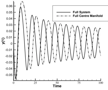
0.00075. The full model was used to compute the solid line and the dot dashed line for the reduced model . . . 48 3.6 Comparison of time histories close to the bifurcation point µ0+

0.00007 . . . 48 3.7 Comparison of time histories far from the bifurcation point µ0+

0.00075.The full model was used to compute the solid line and the dot dashed line for the reduced model . . . 49 4.1 Sparsity patterns for various orderings of the augmented matrix . . . 60

4.2 Convergence histories for TFQMR solution of augmented system

using several preconditioning options . . . 62

(11)

of Iω terms in augmented Jacobian matrix . . . 65 4.4 Fine mesh for NACA0012 aerofoil . . . 70 4.5 Comparison of pressure distribution for NACA0012 aerofoil at zero

incidence and M_∞=0.8 on the coarse and fine grids . . . 70 4.6 Eigenspectrum for quoted values of ¯U , the bifurcation parameter,

on a very coarse grid at a Mach number of 0.5 . . . 71 4.7 Comparison of stability boundaries for the light case on the coarse

and medium grids . . . 72 4.8 Convergence at different Mach numbers for the light case on the

medium grid . . . 73 4.9 Comparison of stability boundary for the light case on the medium

grids with time marching results . . . 74 4.10 Comparison of stability boundaries for the heavy case on the coarse

and medium grids . . . 75 4.11 Comparison of stability boundary for the heavy case on the medium

grids with time marching results . . . 76 5.1 Grid topology (above) and medium surface mesh (below). Note that

only the inner blocks above the wing are shown on the symmetry plane . . . 96 5.2 The variation of flutter speed index with the structural damping

ap-plied at Mach 0.96. The line indicates the measurement . . . 97 5.3 Comparison with measurements of the stability boundaries

calcu-lated on the medium grid using time marching and the bifurcation solver . . . 98 5.4 The convergence of the bifurcation parameter with the bifurcation

solver iteration number at Mach 0.96. The flutter speed index is shown against the right hand axes and the augmented residual against the left hand axes . . . 99 5.5 Number of linear solver steps per bifurcation solver iteration. The

solid line indicates the average number of steps for an aerofoil cal-culation . . . 100

5.6 Comparison of the real and complex formulations for methods 1

and 2 with a modified order Jacobian . . . 101

5.7 Comparison of the real and complex formulations for methods 1

and 2 with a second-order Jacobian . . . 102

5.8 Comparison of complex formulations for all the methods with a

second-order Jacobian . . . 103 5.9 Convergence of flutter speed index for AGARD wing at Mach 0.97 . 104 5.10 Tracking of eigenvalues for AGARD wing at Mach 0.97. Each line

corresponds to one aeroelastic mode and the symbols are consistent between the graphs for the real and imaginary parts . . . 105

(12)

solution at Mach 0.85. Each line corresponds to one aeroelastic mode and the symbols are consistent between the graphs for the real and imaginary parts . . . 106 5.12 Surface pressure distribution and tip aerofoil section for rigid and

static deformed positions of MDO wing at Mach 0.85 . . . 107 6.1 Structural Modes for Goland wing. . . 114

6.2 Behaviour of the damping of modes 2 and 4 for Goland wing at

Mach 0.92. Here dynamic pressure is in units of kg/(msec2). . . 118 6.3 Convergence of bifurcation parameter for Goland wing at Mach 0.92.119 6.4 Comparison between the full and reduced predictions of damping

for Goland wing at Mach 0.92. . . 120

6.5 Comparison between the full and reduced predictions of LCO at

125% of the critical dynamic pressure for Goland wing at Mach 0.92. The symbols are from the simulation of the full system, and the lines are from the reduced model. . . 121 6.6 Growth of the LCO amplitude in the first and second modes at Mach

0.92 for the Goland wing. The filled squares are from the simulation of the full system, and the line is from the reduced model. . . 122 6.7 Response at extremes of the wing at 1.35 times the critical value

of dynamic pressure using the reduced and full models. The unde-flected tip position of the wing is indicated by the blue line joining 2 dots at the wing tip, and the surface contours shown are for change of pressure from the equilibrium value. These results are for the Goland wing at Mach 0.92. . . 123

(13)

List of Tables

2.1 Classification of two dimensional hyperbolic equilibrium points . . 19 2.2 Grid convergence for the solution of the Augmented System . . . . 35 4.1 Structural model parameters . . . 66 5.1 Grid Refinement Influence on Flutter Speed Index at Mach 0.96 . . 87 5.2 Average calculation cost using the PMB code for the first two rows

and the augmented solver for the bottom two rows in the table. The relative costs have been scaled by the time for a steady-state calcu-lation with the appropriate code . . . 87 5.3 Table of the number of non zero in the preconditioner for the

mod-ified order Jacobian . . . 91 5.4 Table of the number of non zero in the preconditioner for the second

order Jacobian . . . 92 6.1 Convergence of reduced order model coefficient real parts under

h refinement. The behaviour of the real and imaginary parts not

shown is identical. Note that all columns include 2nd Jacobian-vector products except the column for G21 which contains a 3rd Jacobian-vector product. The abbreviations d-d and q-d stand for double-double and quad-double respectively . . . 115 6.2 Summary of the costs expressed in multiples of the steady state

solution. . . 119

(14)

Nomenclature

Acronyms

Definition

AIC(s) Aerodynamic Influence Coefficient(s).

BEM Boundary Element Method.

BILU(k) kth Order block incomplete lower upper.

CAE Computational Aeroelasticity.

CFD Computational Fluid Dynamics.

CFD/CSD (coupled) Computational Fluid Dynamics/Computational

Structural Dynamics.

CGS Conjugate Gradients Squared.

CPU Central Processing Unit.

CSD Computational Structural Dynamics.

DES Detached Eddy Simulation.

DLM Doublet-Lattice Method.

FEM Finite Element Method.

GBU Guided Bomb Unit.

GE Gaussian Elimination.

GMRES Generalized Minimal Residual.

HARV High Angle of Attack Research Vehicle.

HB Harmonic Balance.

HDHB High Dimensional Harmonic Balance.

HOHB High Order Harmonic Balance.

ILU Incomplete Lower Upper.

LCOs Limit Cycle Oscillations.

(15)

LEX Leading-Edge Extensions.

LU Lower upper.

NLR Nationaal Lucht- en Ruimtevaartlaboratorium

(Na-tional Aerospace Laboratory of the Netherlands).

NS Navier-Stokes (equations).

ODE Ordinary differential equation.

PIDS Pylon Internal Dispenser System.

PMB Parallel Multiblock Code.

POD Proper Orthogonal Decomposition.

RANS Reynolds-averaged Navier-Stokes (equations).

RCM Reverse Cuthill McGee.

ROM Reduced Order Model.

TFQMR Transpose Free Quasi Minimal Residual.

ZTAIC ZAERO’s Transonic Aerodynamic Influence

Coeffi-cients.

Symbols

Definition

¯ U Reduced velocity = V∞ bωα. w Solution vector.

_{Set of complex numbers.}

ωα Frequency of pitching.

ωh Frequency of plunging.

_{Set of real numbers.}

A Jacobian matrix.

B Second Jacobian matrix.

C Third Jacobian matrix.

i i=√₋1.

M_∞ Mach number.

(16)

A.

Q Matrix whose rows are the left eigenvectors of A.

q Dynamic pressure =1₂ρV2.

R Residual vector.

t Time.

Wc Centre manifold.

p p=pr+ipi The right eigenvector of a matrix.

q q=qr+iqi The left eigenvector of a matrix.

Greek Symbols

Definition

Λ Eigenvalues of a matrix A.

λi The itheigenvalue of the system.

µ Bifurcation parameter.

ω Frequency of the critical eigenvalue.

Subscripts

Definition

f Fluid model.

i Imaginary part of a complex number.

r Real part of a complex number.

s Structural model. d Dynamic solution. qs Quasi-steady solution.

Superscripts

Definition

¯z Complex conjugate. n Dimension of space. T Transpose. t Time level. xv

(17)

Chapter 1

Introduction

Aeroelasticity is the science concerned with the mutual interaction between inertial, elastic and aerodynamic forces[1–3]. Static aeroelasticity arises from the interaction between the inertial and aerodynamic forces, while dynamic aeroelasticity com-prises all three as shown in Figure 1.1 which is called the Collar diagram. The first

Elastic

Force

Inertial

Force

Aerodynamic

Force

Mechanical Vibrations Buzz Flutter Dynamic Response Control Effectiveness Control Reversal

Divergence Dynamic Stability

Flight Mechanics

FIGURE 1.1:Collar diagram - The aeroelastic triangle of forces

recorded flutter incident was on a Handley Page O/400 twin engine biplane bomber in 1916[4]. The flutter mechanism consisted of a coupling of the fuselage torsion mode with an antisymmetric elevator rotation mode. The elevators on this aero-plane were independently actuated and the solution was to interconnect them with a torque tube. Aeroelastic instability (flutter or divergence) can potentially lead to structural failure. This has lead in the aircraft industry to the aeroelastic penalty.

(18)

Solutions to aeroelastic problems generally involve increasing the structural stiff-ness or mass balance, which increases weight while decreasing the performance. The development of aeroelasticity and its effect on design is described in the re-view articles[5, 6]with a survey of more recent applications given by Friedmann[7], Bhatia[8]and Livne[9].

It is argued in Henshaw et al.[10] that more sophisticated aeroelastic mod-elling and prediction will be required in the future compared with the linear methods used today. For example lighter and more structurally efficient designs will reduce stiffness increasing the chances of encountering aeroelastic phenomena. At present flight test programs are used to expand or contract the flight envelope. Problems identified this late in the development cycle may be very expensive to fix. Recently several incidents were reported of cracks in the tail section of the Guided Bomb Unit (GBU) 10 mounted on a Pylon Internal Dispenser System (PIDS) pylon on a F-16. The Royal Netherlands Air Force together with Air Force Seek Eagle Of-fice and National Aerospace Laboratory NLR executed a flight test program to find the cause of the problem[11] which turned out to be high vibration levels in the GBU 10 tail at transonic Mach numbers. The configurations were re-certified with limitations to minimise operation in the transonic regime while the manufacturer was informed of the finding in order to redesign the GBU 10 tail assembly. This is an examine of a limit cycle oscillation (LCO) which is a self sustaining limited amplitude oscillation produced by fluid structure interactions. Both the F-16[12, 13] and F/A-18[14] have encountered LCO at high subsonic and transonic speeds for store configurations with AIM-9 missiles on the wingtips and heavy stores on the outboard pylons.

It is clear that prediction of aeroelastic instability in the transonic regime plays an important role in the definition of the flight envelope for many high per-formance aircraft. Computational Fluid Dynamics (CFD) has matured to become an effective tool for simulating transonic aerodynamics. However, the use of mul-tiple time domain calculations for each aircraft state is computationally expensive and provides limited insight into the dependence of the parameters on the type of response in the vicinity of the instability boundary. This is of particular importance when trying to reconcile anomalous aeroelastic bifurcation phenomena associated with aerodynamic nonlinearities. Consequently there is a need for a systematic and efficient methodology to predict flutter boundaries in the transonic regime,

(19)

sub-sequent LCO responses, and to relate design and operating parameter variations quantitatively to the response characteristics. The methods presented in this thesis are intended to address these points.

1.1

Aeroelastic Prediction

Since the 1950’s[1, 2]aerodynamic strip theory was used in flutter predictions with corrections added to account for compressibility, aspect ratio effects and loss of lift at the wing tips[15]. Aerodynamic strip theory assumes that the strips have no effect on each other, which is valid if the wing is thin and beam like. The inclusion of T-tails required a more advanced method and this was provided via panel methods[16]. The doublet-lattice method (DLM) is a method for modelling the aerodynam-ics of oscillating lifting surfaces. The DLM reduces to the vortex-lattice method at zero reduced frequency. Since it is based on potential flow theory, the DLM cannot describe nonlinear compressible or viscous aerodynamic effects. Industrial flutter analysis[10], using MSC NASTRAN for example, tends to use the DLM, and the linear predictions have been successful as part of an overall process for predict-ing flutter, despite the theoretical limitations. As such they provide an essential point of reference for more sophisticated methods, such as those based on the Euler equations. The output from the DLM is a set of aerodynamic influence coefficients (AICs). The structural model is determined using the finite element method (FEM) with a combination of beam and shell elements. The aerodynamic loads are then coupled to all the structural nodes via spline functions which interpolate the loads onto the structure.

To help improve the capability of the method in the transonic regime it is possible to correct the AICs with unsteady aerodynamic forces. The commercial package ZAERO has the non linear option ZTAIC[17]. The transonic effects are included via a set of steady pressures supplied by the user. These pressures can be from experiments or CFD codes. These pressures are utilised to inverse design an aerofoil shape using the transonic small disturbance equation. The final aerofoil sections then match the user-supplied pressures. Unsteady pressure coefficients on the aerofoil section are then computed by solving the unsteady transonic small disturbance equation.

(20)

cannot predict non-linear effects due to shock waves. As industry moves forward to increasingly lighter designs the risks of flutter and LCO’s playing an important effect increases and this motivates the development of non-linear methods.

1.2

Computational Aeroelasticity

The term computational aeroelasticity (CAE) refers to the coupling of a computa-tional fluid dynamics (CFD) method with a structural dynamics model to perform aeroelastic analysis[7]. The advances in CFD over the last 40 years are well docu-mented. Usable models have increased in fidelity through the transonic small dis-turbance and full potential in the 1970’s, Euler equations in the 1980’s, Reynolds-averaged Navier-Stokes equations (RANS) in the 1990’s and more recently to de-tached eddy simulations (DES) and large eddy simulation (LES). A review of the last 30 years in CFD can be found in Shang[18].

A flutter boundary was obtained for the AGARD wing by solving the un-steady Euler equations of motion coupled to the normal modes of the structure in Lee-Rausch and Batina[19, 20]. The inclusion of viscous effects in the form of the thin layer approximation of the Navier-Stokes (NS) equations was made by the same authors[21] and showed that the inclusion of the viscous terms improved the capture of the transonic dip. Liu et al.[22]presented a coupled code for flutter cal-culations based on a parallel multiblock, multigrid flow solver for the NS equations. The solver was strongly coupled with the structural modal dynamics. This strong coupling allowed for a dual time stepping scheme to be used without a sequencing error. The cost of this type of time domain simulation is not prohibitive when the intention is to examine behaviour at previously identified problem conditions and there are several recent impressive demonstrations of this kind for complete F-16 aircraft configurations (e.g. Farhat et al.[23] and Melville[24]).

CAE has been used to examine a wide range of aeroelastic phenomena. Buf-feting is an instability caused by vortical flow, separation, or shock motions from one part of the aircraft interacting with another part producing a random forced vi-bration. The F-18 high angle of attack research vehicle (HARV) uses wing leading-edge extensions (LEX) to generate vortices which increase wing lift and two ver-tical tail fins which interact with these vortices to enhance maneuverability. At high angles of attack the vortices break down before the tail fins resulting in tail fin

(21)

buffet[25]. Gee et al. used RANS and an overset grid method to calculate the flow around the HARV at high angle of attack[26]. Grid refinement around the fore-body and LEX region improved the prediction of vortex breakdown from previous work. Morton et al.[27] used the commercial version of Cobalt with different turbulence models to predict the position of the vortex breakdown and examined the frequency content at points on the vertical tail. The choice of turbulence model is critical for the prediction of these types of flow with the DES version of Spalart-Almaras com-paring well against the flight-test data. These works were carried out with rigid tail fins and hence no aeroelastic coupling was taken into consideration. Sheta[28] used a multidisciplinary approach to solve the coupled aeroelastic problem to examine the effect of the LEX fences to alleviate tail fin buffet. RANS was used to solve the aerodynamic flowfield and the dynamical response of the tail fin was solved using a direct finite element analysis. The LEX fences shifted the onset of the maximum buffet condition to higher angles and the results compared well to both full scale wing tunnel experiments and flight tests.

Buzz is normally associated with an oscillating control surface in the presents of an oscillating shock. Transonic buzz responses were reported in flight tests on the T45 Goshawk trainer aircraft in the U.S.A.[29] The oscillations were attributed to a shock induced instability and were removed via the use of 2 shock strips. Fuglsang

et al.[29] predicted the location of the shock on the vertical tail fin through steady-state NS calculations with the wings removed. Rampurawala[30] carried out a de-tailed aeroelastic study of this case and found the inclusions of the wings weakened the shock on the vertical tail and hence reduced the buzz. Aileron buzz has also been simulated on the supersonic transport (SST) designed for the National Aerospace Laboratory of Japan. Yang et al. used the thin-layer Navier-Stokes equations cou-pled with the structural equations of motion expressed in modal form to examine the aileron behaviour of two different structural model. The SST structural model which was weakened by reducing the hinge stiffness exhibits aileron oscillations between Mach 0.98 and Mach 1.05.

Divergence is a static aeroelastic phenomena which occurs when the aero-dynamic forces on the wing exceed the elastic restoring forces. Hollowell and Dugundjin investigated the effects of wing bending-torsion stiffness coupling on the divergence speed of unswept lifting surface in incompressible flow[31]. The divergence speed was obtained from the V-g method[1] when both the structural

(22)

damping and frequency abruptly go to zero. The results were in good agreement to low speed wind tunnel tests. They showed that wings with negative stiffness cou-pling exhibited divergence in the first bending mode. Balakrishnan[32] presented an analytical solution to the transonic small disturbance potential equation with the Kutta-Joukowsky boundary conditions for a zero thickness aerofoil at non-zero an-gle of attack. The resulting equation for the divergence speed showed explicitly a transonic dip dependant on the angle of attack.

If the flow about a lifting surface becomes partial or completely separated during any part of the periodic oscillation then the instability is called stall flutter. Stall flutter is normally associated with compressor cascades in turbojets and he-licopter rotor blades. Datta and Chopra used a loosely coupled RANS code and structural model on a single UH-60A blade to show the first stall cycle was caused by high trim angles in the retreating blade while the second stall cycle was caused by the elastic twist[33].

There has been recent interest in the LCO behaviour of wing store config-urations. Store induced LCOs have been simulated for the rectangular Goland+

wing[34, 35]. The aeroelastic solver was developed by integrating a modal structural

model from MSC/NASTRAN with the commercial CFD solver FLUENT. A spline matrix was used to transfer data from the non matching aerodynamic grid and struc-tural grid. Store aerodynamics were found to affect the LCOs in two ways first be adding loads to the structure and secondly by interfering with the flow over the wing.

As a prelude to the work reported in this these, the parallel multiblock code[36] (PMB) was extended to allow CAE computations. A number of considerations were required

(a) The movement of the CFD grid by transfinite interpolation.[19, 37] (b) Sequencing in time between the CFD/CSD solutions.[38, 39] (c) The intergrid transfer of data.[40, 41]

Time domain flutter predictions have been obtained with PMB for problems ranging from model wings[42] to in production aircraft[43].

Time-domain methods are general and have been shown to accurately pre-dict non linear effects. Despite the significant gains in algorithm efficiency and raw computing power, which has reduced the computational cost of time response cal-culations of complete aircraft down to a few hours[43], they remain too costly for

(23)

routine prediction of flutter boundaries and LCO amplitude prediction. Multiple calculations must be undertaken across the flight envelope to find the flutter point and the LCO behaviour. This has motivated a research effort to search for methods which account for nonlinear effects but at a much reduced computational cost.

1.3

Reduced Order Modelling

Reduced order model (ROM) or low dimensional approximations to a large system of equations greatly reduces both the central processing unit (CPU) cost and stor-age requirements of aeroelastic calculations. These models are vital for parametric studies, optimisation of structures and control problems. However, to be useful, they must be capable of reproducing the important linear and non-linear behaviour of the full system.

There are two approaches to model reduction. System identification methods take the response of the system to inputs and use this information to build a low order model. The second method is to manipulate the full order system to reduce the cost of calculations. In this thesis the second class of method will be consid-ered. More comprehensively, the review papers of Dowell and Hall[44] and Lucia, Beran and Silva[45] examine a number of techniques which include proper orthog-onal decomposition (POD), Volterra series, the harmonic balance method, and an eigenmode method.

1.3.1

The Eigenmode Methodology

Hall[46]constructed ROM’s using an unsteady vortex lattice method which assumes the flow to be incompressible, inviscid and irrotational. Consider the iterative scheme

Awt+1+Bwt=Rt+1 (1.1)

where w is the solution, t is the time level and R is the residual. Consider the homogeneous part of (1.1) then the generalised eigenvalue problem is

APΛ+BP=0 (1.2)

where Λ is a diagonal matrix of order N containing the eigenvalues and P is an

N_×N matrix whose columns are the right eigenvectors. Analogously

(24)

where Q is a N_×N matrix whose rows are the left eigenvectors. These eigenvectors

can be scaled to satisfy the following orthogonality conditions

QTAP=I, QTBP+Λ=0. (1.4)

Then the dynamic behaviour of the system can be determined by using the mode superposition method by representing the response as the sum of all the eigenvectors

w=Pc (1.5)

where c is the vector of normal mode coordinates for the eigenmodes. Substituting equation (1.5) into (1.1) and using the orthogonality conditions equation (1.4) yields

N uncoupled equations

ct+1₋Λcn=QTRt+1. (1.6)

The ROM is now constructed by keeping only a few of the original modes. A static correction technique is often required to improve the ROM to give satisfactory results[46, 47].

Static correction is applied by decomposing the unsteady solution into the response of the system if the disturbance is quasi-steady, and the dynamic part

wt=wt_qs+wt_d=wt_qs+P ˆct. (1.7)

The quasi-steady part wn_qsis given by

(A+B)wt_qs=Rt (1.8)

and hence the corrected ROM is ˆ

ct+1₋Λcˆt =QTRt+1₋QT(Awt_qs+1+Bwt_qs). (1.9) Hall used this model on a rectangular wing of aspect ratio 5 to reduce the number of degrees of freedom from 480 to 40. He showed that without the static correction 40 modes is not adequate to capture the behaviour at high reduced fre-quencies. For fluid models where the dimension of the eigenvalue matrix is of the order 104 it is possible to use a standard eigensolver package to obtain the eigen-values. Romanowski and Dowell[48], applied this ROM to subsonic unsteady flows around the NACA 0012 aerofoil, based on the Euler equations. The eigenvalue problem was solved using the Lanczos method[49]. It has been shown that the exis-tence of zero eigenvalues in the eigensystem is the main reason for needing to apply

(25)

a static correction technique. Hence Shahverdi et al.[50] constructed a reduced-order model based only on the wake eigenmodes with, the body quasi-static eigen-modes removed. They applied this technique for unsteady flow computations based on the boundary element method (BEM). When the Prandtl-Glauert compressibility correction is used to consider linear compressibility effects the results were in good agreement to the Euler solutions[48].

This methodology cannot easily be extended to the three dimensional Euler equations since it is very expensive to calculate eigenvalues when the order of the matrix is above 104.

1.3.2

Proper Orthogonal Decomposition

Proper orthogonal decomposition (POD) is a modal method applicable to systems for which multiple measurements are simultaneously available. Early application was to the analysis of experimental data with a view to extracting trends and dom-inant features[51]. In the aeroelastic context POD is applied to a matrix of multiple measurement locations sampled through time. POD can help determine the number of active modes in an oscillatory system and can be used as an optimal representa-tion of the form of the modes and hence is used to construct reduced order models [52]_{. This method has been successfully applied to a wide range of problems} includ-ing complete aircraft configurations[53, 54].

A POD basis,Φ=

e1,e2,e3, . . . ,ej

is orthogonal and can be used in a modal decomposition w(t)_≈W0+ M

∑

j=1 ˆ wi(t)ei=W0+Φwˆ(t) (1.10) where ˆw is the vector of modal amplitudes, W0 is some baseline solution and M is the number of modes.

For dynamical problems the POD modes are constructed by first computing a number of snapshots of the full order system response in time,

S=

W1,W2,W3, . . . ,Wn (1.11) A new basis is formed from the linear transformation of the snapshot matrix S

(26)

and maximising the projection of the snapshot matrix onto the POD basis yields the following eigenvalue problem

STSV =VΛ. (1.13)

The eigenvalues satisfyλi_≥0 since STS is symmetric positive semi-definite. The

eigenvectors V are normalised so that VTV =I, and then scaling eibyλ_i−1/2gives

an orthonormal set of modes, i.e. ΦTΦ=I.

In practise fewer that M modes are retained. This is done by limiting the set to only the eigenvectors corresponding to sufficiently large eigenvalues. A property of this decomposition is that it minimises the approximation error when a member of the class S is approximated through a linear projection onto M basis vectors[51].

There are a number of different techniques for obtaining a set of reduced order equations for w(t) with different projections. These have recently been re-viewed in Lucia et al.[45]. The data samples for a POD are collected over a small region of state space, this focused sampling allows for very accurate ROM at the training point. However a ROM is not usually robust with respect to changes in the model parameter[55]. Ideally the ROM should be reconstructed whenever the model parameter is changed. To avoid this CPU intensive effect recently ROM adapta-tion techniques have been used. There are at least 4 different techniques used in aerospace problems:

(1) The global POD (GPOD)[56] which has only been demonstrated to be effective at low free stream Mach numbers.

(2) The method of direct interpolation of the reduced order basis vectors[57] which has delivered poor results in the transonic regime because the vectors vary non linearly with Mach number and angle of attack.

(3) The subspace angle interpolation[57, 58]adapts two ROMs associated with two different sets of model parameters to a third set by interpolating between the basis rather than the vectors of the basis. Lieu showed that the principal angles between subspaces of 2 ROMs appear to vary linearly for subsonic Mach numbers for intervals of 0.2 of a Mach number, this interval is halved in the transonic regime. Hence the adapted ROMs do a reasonable job of predicting transonic flow if there is enough ROMs throughout the Mach number range.

(4) The final interpolation method based on the Grassmann manifold, its tan-gent space at a point and the computation of geodesic paths[59]. The Grassmann manifoldG₍_k_,_n₎_{is a space which parameterises all linear k-dimensional subspaces}

(27)

of an n-dimensional vector space i.e. G₍₂_,₃₎ _{is the space of all planes that pass}

through the origin. The last two methods are closely linked as a two point Grass-mann manifold corresponds to a subspace angle interpolation.

The generation of the training data is still costly as unsteady CFD compu-tations must be undertaken. More importantly it is also very difficult to produce a ROM and at present there are no POD aeroelastic results for viscous full order models.

1.3.3

Harmonic Balance Method

The formulation of the harmonic balance (HB) method of Hall et al.[60], yields an efficient method for the calculation of time periodic solutions of large non linear systems of equations. The semi-discrete form of the system of ordinary differential equations is

I(t) = dw(t)

dt +R(t) =0. (1.14)

Assume that the solution and residual are periodic in time with frequencyω. Then they can be expanded in a Fourier series which is truncated to NH terms as

w(t)_≈wˆ0+ NH

∑

n=1 (wˆancos(ωnt) +wˆbnsin(ωnt)) (1.15) R(t)_≈_Rˆ₀₊ NH

∑

n=1 ˆ Rancos(ωnt) +Rˆbnsin(ωnt) (1.16) The expansions (1.15) and (1.16) are then substituted into the the original governing equations (1.14) to give a system of equations for the unknown harmonic terms,

ˆ

R0 = 0

ωn ˆwbn + Rˆan = 0

−ωn ˆwan + Rˆbn = 0

(1.17)

The difficulty in solving the system of equations (1.17) is in finding a relationship between the solution and residual in the frequency domain. To avoid this problem the system is converted back into the time domain. The solution is split into 2NH+1

discrete equally spaced sub-intervals

W=        w(t0+∆t) w(t0+2∆t) .. . w(t0+T)        R=        R(t0+∆t) R(t0+2∆t) .. . R(t0+T)        (1.18)

(28)

where∆t=2π/(ω(2NH+1)). There exists a transformation matrix E such that

ˆ

W=EW and Rˆ =ER. (1.19)

and then the system of equations (1.17) can be written as

ωDW+R=0 (1.20)

where D is a 2NH+1×2NH+1 matrix of the form

Di,j= 2 2NH+1 NH

∑

k=1 k sin(2πk(j₋i)/(2NH+1) (1.21)

The standard pseudo-time steady-state approach to solving the HB equation (1.20) can be applied. So, in effect, by using the truncated periodic solution the unsteady problem has been converted into a 2N+1 steady state problem. Good results have been claimed with even a small number of modes when modelling the LCO be-haviour of the F-16[61]. This method is closely related to the non-linear frequency domain methods of McMullen et al.[62, 63]. They employ a very similar approach but solve the system of equations (1.17) in the frequency domain. Assuming ˆW

is known, the time domain solution can be constructed. The steady-state residual operator R is then applied to each of these time instances and these are converted back into the frequency domain via a fast Fourier transform. McMullen et al. also derive a gradient approach for the class of problems where the time period is not known a priori[63]. An iterative approach is used which adjusts the time period at each iteration by using the derivate of the square of the residual in the frequency domain with respect to T as the correction.

Two HB formulations have been analysed in detail for Duffing’s oscillator in Liu et al.[64], the formulation by Hall was denoted as the high-dimensional har-monic balance (HDHB) method due to its applicability for high-dimensional dy-namical systems. It was shown that the HDHB system always contains more terms than the classical HB system for the same number of harmonics. These extra terms have the effect of producing non physical solutions and may increase the number of harmonics required for a given accuracy. Maple et al. introduced an adaptive harmonic balance[65, 66]to reduce the computational cost further. Each cell was ex-amined to see what fraction of spectral energy contained in the highest computed Fourier frequency and refined if they exceed a threshold value. It was shown to

(29)

work well for supersonic/subsonic diverging nozzle where the periodic solution is mostly continuous and low frequency but with a shocked region.

The cost of mapping a stability boundary by the HB could be substantial. If it is not known a priori which modes interact, then there is no estimate of what frequency ω is required in (1.15) and (1.16). So a number of calculations will be required to explore the frequency domain. A flow containing highly non-linear features that need to resolved accurately, e.g. shocks, will require a large number of modes for each calculation at added further computational cost.

1.4

Dynamical Systems Based Methods

In CAE the partial differential equations are turned into a system of ordinary differ-ential equations, making it logical to appeal to dynamical systems theory in order to calculate flutter boundaries and predict LCOs. The goal of this thesis is to take these standard ideas and turn them into practical methods that can be used to solve large aeroelastic systems.

1.4.1

Numerical Analysis of Bifurcations Points

Bifurcation theory is the study of changes in the qualitative behaviour or topologi-cal structure of a given problem. A bifurcation occurs when a small smooth change in a parameter(s) leads to a sudden topological change in system behaviour. Given a set of ordinary differential equations depending on a set of parameters the idea is to obtain its bifurcation diagram. These diagrams divide the parameter space into regions within which the system has topologically equivalent behaviour. Dy-namic pressure vs Mach number and flutter speed index vs Mach number are two common diagrams in aeroelastics. These regions for aeroelastic systems include: stable - all modes are damped, unstable - there is at least one divergent mode, or LCOs. All these regions have been shown on the rectangular Goland wing model with tip store[67]. For a fixed Mach number as the velocity is increased the wing passes from being stable to being unstable at around 650 ft/sec. However between Mach 0.92 and Mach 0.94 there is a small pocket of LCOs at a velocity of 450 ft/sec. Mapping the boundaries where the system flips from one region to another is important. Other information of interest is how fast the modes are damped in the

(30)

stable regions and the amplitude of any LCOs. All these questions can be answered with time marching CAE, but at the expense of significant computer time.

1.4.2

Calculation of Bifurcation Points

The first part of mapping out the behaviour of a system of ODEs is to calculate the equilibrium points where the system switches behaviour. Consider the system of non-linear ordinary differential equations

˙x= f(x,µ) x_∈n µ _∈ _(1.22)

where µ is the bifurcation parameter. The equilibrium points of equation (1.22) satisfies

f(x,µ) =0. (1.23)

The system switching behaviour is characterised by a change in the eigenvalues of the Jacobian matrix

A= fx(x,µ). (1.24)

For example if all the eigenvalues of A have negative real part then the equilibrium point is stable. In the case of a simple LCO the Jacobian matrix has a complex pair of eigenvalues valuesλ =λr+iλi withλr >0 andλi₆=0 with all other eigenval-ues having negative real part. The boundary for the change in behaviour between a stable equilibrium point and an LCO is when a complex pair of eigenvalues crosses the real axis. This bifurcation point is called a Hopf bifurcation. Seydel[68] di-vided methods for locating bifurcation points into two classes indirect and direct methods. For indirect methods a bifurcation point is calculated by solving equa-tion (1.23) repeatedly for different values of µ and detecting a change of sign of a test function which classifies the bifurcation point. For the Hopf bifurcation one possible test is to calculate all the eigenvalues of (1.24) and see when one pair crosses the real axis[68]. When the crossing has been detected the secant method can be used to solve for the real part of λ is zero[69]. The direct methods solve the system of equations (1.23) augmented by additional equations that characterise the bifurcation point. Roose[70] proposed a direct method for the computation of Hopf bifurcations which was to solve a augmented system of dimension 2n+2. Griewank and Reddien[71] developed a similar method which solves a system of dimension 3n+2. Holdniok and Kubiˇcek[72] compared 4 different methods two of

(31)

which required the evaluation of the coefficients of the characteristic polynomial of the Jacobian matrix.

1.4.3

Normal Forms for Bifurcations

The normal form of a bifurcation is a simplified system of equations that approx-imates the dynamics of the system in the vicinity of a bifurcation point. The simplification can be obtained by using a number of methods, i.e. centre man-ifold reduction[73], the Lyapunov-Schmidt method[74] and the method of multiple scales[75, 76]. The dimension of the normal form is generally much lower than the di-mension of the full system of equations. For a Hopf bifurcation the normal form is a two-dimensional system.[77]Dessi and Mastroddi[78] have used the method of mul-tiple scales to examine a three degree of freedom airfoil flap configuration with two non-linear torsional springs (cubic) in two-dimensional incompressible flow. Vio

et al.[79] applied a number of bifurcation analysis techniques to the transverse gal-loping of a square sectioned beam in a normal steady flow. The aerodynamic force was expressed as a seventh order polynomial function of velocity and the struc-ture as a mass with linear stiffness and non-linear damping. The methods used in the study included centre manifold[80], normal form[81], numerical continuation[82] and higher order harmonic balance[83] (HOHB). Only two of the methods exam-ined, namely HOHB and Numerical continuation where able to fully and accurately characterise the problem.

1.5

Thesis Outline

This thesis is concerned with the development of fast methods for the prediction of flutter boundaries and LCO responses in transonic flow. To this end the Euler equations are used to capture the changing behaviour of shocks in response to the motion of the aircraft. An a priori assumption is made on the dynamics of the flutter, namely that it is a Hopf Bifurcation which signals a change from stable steady motion to periodic motion.

Chapter 2 summarises the theory of Hopf bifurcations and methods that can detect when such a bifurcation has been encountered. The formulation is extended and used to calculate the value of a single parameter for which an eigenvalue of the

(32)

system Jacobian matrix crosses the imaginary axis. The chapter concludes with a model example of a 1D tubular reactor.

Whilst knowledge of the onset of the instability is important more informa-tion is required in practice. For example the fast comparison of predicinforma-tions and flight test damping data is required to inform decisions about future test points dur-ing flight testdur-ing. If the stability boundary is crossed in flight, knowledge of the LCO amplitude is required. Chapter 3 contains the theory of centre manifold pro-jections and highlights some of the difficulties involved in using such a method when the system of equations is of the order 106. The chapter concludes again with a model example of a 1D tubular reactor.

In chapter 4 the method outlined in chapter 2 is developed into a scheme that is applicable to the two dimensional Euler equations coupled with a pitch-plunge dynamics model. The method shows a two orders of magnitude reduction in CPU time to calculate a flutter boundary compared with time-marching.

Chapter 5 takes the method of chapter 4 and demonstrates it on three di-mensional test cases. It is shown that the method has reached a sufficient level of maturity that it has been used on real aircraft problems within the research activities of industry[10].

In chapter 6 the theory outlined in chapter 3 is turned into a practical method for calculating the damping and limit cycle oscillations for wings. The method uses information obtained from the approach of chapter 5 to reduce the system of equations down to 2 degrees of freedom. This allows for near instantaneous calculation of LCO responses once the model is formed.

The methods presented in chapters 4-6 provide a unique and powerful set of tools for exploiting the modelling capability of CAE. An important feature of the work is the demonstration of the methods that can be applied to problems of realistic size. These methods have all been published in journal papers listed at the start of the thesis.

(33)

Chapter 2

Calculation of Hopf Bifurcation

Points

2.1

Introduction

Recent studies by Morton and Beran[84, 85]suggest that, for a large class of transonic aeroelastic problems, a more direct evaluation of the critical stability boundary is feasible, based on numerical path following techniques[68] and the augmented sys-tem of Griewank and Reddien[71]. Here, the parameterised aeroelastic equations of motion are expressed notionally in semi-discrete form. Local bifurcations of equi-libria are associated with degenerate behaviour of the linearised aeroelastic equa-tions in which one or more of the eigenvalues of the Jacobian matrix (1.24) has zero real part. For example, the onset of LCO, at which a steady-state solution transitions to an oscillatory solution with zero amplitude under the influence of a single param-eter, can be identified with a simple Hopf bifurcation in which the Jacobian matrix possesses a conjugate pair of pure imaginary eigenvalues with non-zero frequency. These are the critical eigenvalues.

Under the variation of multiple parameters, more complex degeneracies are possible. The degree of degeneracy (or co-dimension) of a critical point is defined by the minimum number of parameters required to fully explore the qualitatively distinct solution behaviour in the vicinity of the critical point. Numerical path fol-lowing (continuation) techniques enable particular degeneracies of steady state so-lutions of prescribed co-dimension to be tracked with respect to the free-stream and structural parameters, thereby identifying directly critical stability boundaries

(34)

in parameter space. From a knowledge of the type of degeneracy at criticality it is possible to infer qualitatively generic local bifurcation characteristics[86]. In addi-tion, the critical eigensolutions associated with the degenerate Jacobian matrix are automatically determined as an integral part of the procedure, thereby providing insight into the composition of the critical aeroelastic modes. This modal infor-mation also forms the basis of quantitative model reduction procedures[87] which can be used to explore sub- and post-critical behaviour in the neighbourhood of the critical bifurcation parameters.

Of practical importance, direct path-following methods generally demand less computational effort than existing time-integration procedures for the evalu-ation of stability boundaries whilst offering additional informevalu-ation in the sub- and post-critical aeroelastic behaviour over a range of parameters in the vicinity of crit-icality. The approach operates directly on the semi-discrete CFD/CSD representa-tion of the aeroelastic system. Moreover, the direct approach is not limited to the prediction of simple nonlinear flutter phenomena but can incorporate aeroelastic be-haviour associated with higher-order degeneracies and multiple critical eigenvalues such as the double Hopf bifurcation which has been observed on a single degree of freedom bluff body with a tuned mass damper[88].

2.2

One Parameter Bifurcation Equilibria

Consider a continuous time system depending on a parameterµ ˙

w= f(w,µ), w_∈n_, µ_∈_, _(2.1)

where f is smooth with respect to both w andµ. The eigenvalues of the Jacobian matrix ∂f/∂w, are important for determining the stability characteristics of the

equilibria of the system. Let x =x0 be a hyperbolic equilibrium1 point of the system forµ =µ0. Consider the two dimensional n=2 system then the Jacobian matrix has either two real eigenvalues λ1 and λ2 or one complex conjugate pair

λ1,2=λr±iλi. There are 3 topological classes of hyperbolic equilibrium for this system,[87] namely nodes, saddles and foci. These are distinguished by the positive and negative real parts of the eigenvalues, see Table 2.1.

(35)

Real λ1≤λ2<0 Node stable

Real 0<λ1≤λ2 Node unstable

Real λ1<0<λ2 Saddle unstable

Complex λr <0 Focus stable

Complex λr >0 Focus unstable

TABLE 2.1:Classification of two dimensional hyperbolic equilibrium points

There are only two ways in which the hyperbolicity condition can be violated. Either a simple real eigenvalue approaches zero hence λ1=0, or a pair of simple complex eigenvalues reach the imaginary axis andλ1,2=±iω0, ω0>0 for some value of the parameter. It can be shown that more than one parameter is required to allocate extra eigenvalues on the imaginary axis.[87]

For one parameter bifurcations only two of these types are possible. The first is called a fold and is associated with the appearance of a zero eigenvalue. This is also referred to as a limit point or a turning point. The one-dimensional system

f(w,µ) =µ+w2

is the simplest possible system that has an equilibrium point at(0,0)and satisfies the fold bifurcation condition fx(0,0) =0. The second type is the Hopf bifurcation

which is associated with the appearance of a purely imaginary eigenvalue.

2.3

Classes of Hopf Bifurcation

Consider the following system of two differential equations depending on one pa-rameterµ

˙

w1 = µw1−w2−w1(w21+w22), ˙

w2 = w1+µw2−w2(w21+w22). (2.2)

This system is the simplest possible that exhibits a Hopf bifurcation. This system has the equilibrium w1=w2=0 for allµ with the Jacobian matrix

A= µ −1

1 µ

(36)

having eigenvaluesλ1,2=µ±i. If the complex variable z=w1+iw2is introduced, then the complex conjugate is given by ¯z=w1−iw2, and the magnitude|z|2=z¯z= x2₁+x2₂. This variable satisfies the differential equation

˙z=w˙1+i ˙w2=µ(w1+iw2) +i(w1+iw2)−(w1+iw2)(w21+w22), and equation (2.2) can be rewritten in the complex form

˙z= (µ+i)z₋z_|z_|2. With the change of variable z=reiθ then

˙z=˙reiθ+ri ˙θeiθ =reiθ(µ+i₋r2). which gives the polar form of equation (2.2).

˙r = r(µ₋r2)

˙

θ = 1. (2.3)

Bifurcations of the phase portrait of the system asµ passes through zero can easily be analysed using this polar form since the equations for r andθ decouple. Since r_≥0 the first equation has the equilibrium point r=0 for all values ofµ. The equilibrium is linearly stable if µ <0, nonlinearly stable for µ =0, and linearly unstable for µ >0. There is an additional stable point r0(µ) =√µ for µ > 0. The second equation describes a rotation with constant speed. Taking these two pieces of information the following description of the bifurcation behaviour can be obtained.

The behaviour of the system can be seen in Figure 2.1. The system always has an equilibrium point at the origin. This is a stable focus for µ <0 and an un-stable focus forµ >0. At the critical value ofµ =0 the equilibrium is nonlinearly stable and topologically equivalent to the focus. This equilibrium at the origin is surrounded by an isolated closed orbit (limit cycle) that is unique and stable ifµ>0. The cycle is a circle of radius r0(µ) =√µ. All orbits starting outside or inside the circle (with the exception of the origin) tend to this cycle as t _→+∞. There is a Hopf bifurcation atµ =0.

A system having nonlinear terms with the opposite sign to equation (2.2) ˙

w1 = µw1−w2+w1(w21+w22), ˙

(37)

w2 w1 w2 w1 w2 w1 µ=₋0.10 µ =0.0 µ =0.15

FIGURE2.1: A supercritical Hopf bifurcation in the plane

has the following complex form

˙z= (µ+i)z+z_|z_|2.

which can be analysed as above. The system passes through a Hopf bifurcation at

µ =0. Since the nonlinear terms are of opposite sign to equation (2.2) there is an unstable limit cycle in equation (2.4) as can be seen in Figure 2.2.

There are two types of Hopf bifurcation. The bifurcation in system (2.2) is called a supercritical bifurcation because a stable equilibrium exists before bifur-cation and a stable limit cycle after. The bifurbifur-cation in system (2.4) is called a subcritical bifurcation because an unstable limit cycle exits before the bifurcation and an unstable equilibrium solution after.

If higher order terms are added to equation (2.2) and written in a vector form then ˙ w1 ˙ w2 ! = µ −1 1 µ ! w1 w2 ! −(w2₁+w2₂) w1 w2 ! +O₍_||_w_||4₎ _(2.5)

where w= (w1,w2)T, ||w||2=w2₁+w2₂, andO(||w||4)terms can smoothly depend on µ. The system (2.5) is locally topologically equivalent near the origin to sys-tem (2.2) and the higher order terms do not effect the bifurcation behaviour of the system.

(38)

w2 w1 w2 w1 w2 w1 µ=₋0.15 µ =0.0 µ =0.10

FIGURE2.2: A subcritical Hopf bifurcation in the plane

2.4

Numerical Methods for Calculating Equilibrium

Solutions

The calculation of an equilibrium solution requires the solution of a nonlinear sys-tem of algebraic equations (2.1) for a given µ. An attractive method for achieving this is Newton’s method, or a variant. For clarityµhas been dropped in the methods are outlined below.

2.4.1

Newton’s Method

Let A(w) =∂f/∂w denote the Jacobian matrix of f evaluated at a point w. Suppose wtis the current approximation to the solution of equation (2.1). If we linearise the left hand side of equation (2.1) near wtthen

f(wt) +A(wt)(wt+1₋wt)_≈0.

If the matrix A(wt)is invertible this linear system will have the solution

wt+1=wt₋A−1(wt)f(wt), (2.6)

which should be closer to w0 than wt. Let w0 be a given initial point near the equilibrium point w. Then Newton’s iteration is defined by the recurrence relation

(39)

(2.6). It should be noted that matrix A(wt)need not be inverted to compute wt+1but equation (2.6) must be solved. If the Jacobian has a special structure, for example sparse, it is very useful to take this into account.

Suppose the system (2.1) is smooth and has an equilibrium w0 at which no eigenvalue is zero in the Jacobian matrix. Then there is a neighbourhoodW _{of w}₀

so that the Newton iterations converge to w0from any initial point w0∈W and

kwt+1₋w0k ≤κ0kwt−w0k2, t=0,1,2, . . . (2.7) for someκ0>0. A practical method is however needed to obtain an initial guess which is withinW_{. The convergence of this method is independent of the stability}

of the equilibrium since the no zero eigenvalues in the Jacobian matrix is equivalent to equation (2.6) having a solution. The estimate above means that the error is approximately squared from one iteration to the next, giving the famous quadratic convergence.

2.4.2

Relaxed Newton’s Method

Newton’s method requires that the initial guess w0 is close, in some sense, to the equilibrium solution w0. Newton’s method can be modified to increase this domain of convergence at the expense of reducing the rate of convergence by adding a time-like term onto the diagonal of the Jacobian matrix so that

( 1

∆TI+A(w

t₎₎₍_wt+1

−wt) =₋f(wt). (2.8)

The term ∆T can be a physical time step or can be adjusted locally to accelerate

convergence. As the time step is increased the pure Newton’s method, and quadratic convergence, is recovered.

2.4.3

Modified Newton’s Methods

If no analytical formula for the Jacobian matrix is available then an expensive eval-uation by numerical differentiation is required. Some approximations may be pos-sible to reduce the required cost, as for example is done in some CFD codes[89].

One possible simplification is to freeze the Jacobian matrix at the initial value. This is called the Newton chord method. This simple idea gives rise to the iteration

(40)

whereδwt is now given by

A(w0)δwt =₋f(wt). (2.9)

This also converges to w0but at a rate given by

kwt+1₋w0k ≤κ1kwt−w0k, t =0,1,2, . . . (2.10) for some 0<κ1<1. Hence the convergence is only linear.[90]

The Broyden[91] update is a member of a family of methods which use rank one updates, that is At+1₋Atis a matrix of only one linearly independent row. The idea is that two successive iterates and the corresponding function values are used to update the matrix involved in the computation of δw. Broyden’s method is a

generalisation of the secant method when applied to the Jacobian matrix A

At+1(wt+1₋wt)_≈F(wt+1)₋F(wt). (2.11) Unless the dimension of w is one this equation is under determined. Broyden sug-gested using a rank one update of At to calculate At+1

At+1=At+uvT (2.12)

where u,v_∈n_{. Requiring that A}t+1_r₌_At_{r for all r orthogonal to w}t+1₋_wt _and

using equation (2.11) implies

v=wt+1₋wt u= F(w

t+1₎₋_F₍_wt₎₋_At₍_wt+1₋_wt₎

(wt+1₋_wt₎_·₍_wt+1₋_wt₎ .

This gives rise to the following algorithm, starting with an initial guess w0 and an estimate of the Jacobian matrix A0then

wt+1 = wt₋(At)−1F(wt) st = wt+1₋wt yt = F(wt+1)₋F(wt) At+1 = At+(y t₋_At_st₎₍_st₎T st_·_st

for t=1,2,3, . . .. Better convergence than the Newton chord method is obtained[92] but there is no expectation that At converges to the Jacobian matrix A(w0) at the equilibrium point w0, even if the method converges to w0 as t →∞. Hence, the final matrix cannot be used to compute, say, the eigenvalues of A at w0. Normally the Jacobian matrix A(w)has a special structure (for CFD methods, this is banded and sparse) and this is always used to allow efficient linear solution. However the rank one update of Broyden’s method may not preserve this structure.

(41)

2.5

Numerical Methods for Calculating Hopf

Bifur-cations

Consider the continuous time system (2.1) depending upon one parameter µ. An equilibrium solution satisfies

<

Fast prediction of transonic aeroelasticity using computational fluid dynamics

Woodgate, Mark A. (2008)

study, without prior permission or charge

When referring to this work, full bibliographic details including the

Declaration

Acknowledgements

List of Most Relevant Publications

Contents

Abstract iii

List of Figures

List of Tables

Nomenclature

Symbols

Greek Symbols

Definition

Force

Aeroelastic Prediction

Computational Aeroelasticity

Reduced Order Modelling

QTAP=I, QTBP+Λ=0. (1.4)

Proper Orthogonal Decomposition

STSV =VΛ. (1.13)

Harmonic Balance Method

Dynamical Systems Based Methods

Calculation of Bifurcation Points

Normal Forms for Bifurcations

Chapter 2

One Parameter Bifurcation Equilibria

Classes of Hopf Bifurcation

Numerical Methods for Calculating Equilibrium

Relaxed Newton’s Method

Modified Newton’s Methods

Numerical Methods for Calculating Hopf