Flow characterisation for a validation study in
high-speed aerodynamics
Kshitij Sabnis
∗and Holger Babinsky
†Department of Engineering, University of Cambridge, Cambridge, CB2 1PZ, UK
Daniel S. Galbraith
‡and John A. Benek
§Air Force Research Laboratory, Wright-Patterson AFB, Ohio, United States
Validation studies are becoming increasingly relevant when investigating complex flow problems in high-speed aerodynamics. These investigations require calibration of numer-ical models with accurate data from the physnumer-ical wind tunnel being studied. This paper presents the characterisation process for a joint experimental-computational study to inves-tigate the streamwise corners of a Mach 2.5 channel flow. As well as checks of flow quality typically performed for phenomenological investigations, additional quantitative tests are conducted. The extra care to obtain high quality data and eliminate any systematic errors reveal useful information about the wind tunnel flow. Further important physical insights are gained from designing and conducting wind tunnel tests in conjunction with numeri-cal simulations. Crucially, the close experimental-computational collaboration enabled the identification of secondary flows in the sidewall boundary-layers; these strongly influence the flow in the corner regions, the target of the validation study.
Nomenclature
H shape factor M Mach number p pressure P r Prandtl number T temperature u streamwise velocity v floor-normal velocity w spanwise velocity x streamwise coordinate(measured from nozzle exit) y floor-normal coordinate
(measured from tunnel floor) z spanwise coordinate
(measured from tunnel centre span) δ boundary-layer thickness
(99% of freestream velocity) δ∗ displacement thickness
θ momentum thickness
Subscript
i equivalent incompressible quantity 0 stagnation property
0s settling chamber stagnation property 02 Pitot-measured property
∞ freestream property
Superscript
+ quantity expressed in non-dimensional wall units
Abbreviations
CAD computer-aided design CFD computational fluid dynamics HLLC Harten-Lax-van Leer-Contact LDV laser Doppler velocimetry RANS Reynolds-averaged Navier Stokes SSOR symmetric successive over-relaxation
∗PhD Student, Department of Engineering, University of Cambridge.
†Professor in Aerodynamics, Department of Engineering, University of Cambridge, AIAA Associate Fellow. ‡Engineer, Computational Sciences Centre, AFRL Aerospace Systems Directorate.
I.
Introduction
The computational modelling of flows has enjoyed great advance over recent years, progressing from basic numerical algorithms of simple physical cases to the design of sophisticated real-life systems. The field has now reached a stage, however, where it is necessary to test models with highly accurate experimental data in order to further extend the capabilities of simulations. Furthermore, for complex flow problems, simply using experiments or numerical methods alone is insufficient to probe the underlying fluid mechanics; the two approaches need to be employed in conjunction to extend our physical understanding.
One key area with a pressing requirement for validation studies is that of supersonic corner flows. Sepa-ration in streamwise corners is a pervasive problem in high-speed flows, contributing 4–6% to the total drag of fighter aircraft.1 However, there are still no consistently successful techniques to mitigate separation in the corners.2, 3 Computational costs often limit simulations in real-world applications to RANS methods, but these are not able to reliably predict corner flows. This is compounded by the notable lack of reference data for these geometries, even without shock-induced adverse pressure gradients. This absence of suit-able experimental data presents a major obstacle to the development of relevant computational methods. In turn, the inadequacy of modelling techniques inhibits our understanding of corner flows and ability to predict separation features.
The combined experimental-computational study presented in this paper aims to address the lack of information on this topic by investigating the flow in the corner of a supersonic channel flow with no adverse pressure gradient. Experiments can typically be divided into two categories: science discovery investigations, which aim to deepen understanding of the flow physics, and validation studies, which help to determine the accuracy and limitations of numerical models. This work falls under the latter category.
The methodology is designed specifically to characterise the wind tunnel and calibrate computational models of the flow. It is now accepted that a perfect wind tunnel is near-impossible to build and run; instead, the emphasis is placed on carefully measuring the “imperfections” of the physical wind tunnel so that computations can accurately reproduce the true flow. Performing these characterisation tests with the aim of calibrating numerical simulations demands a more detailed focus on experimental accuracy than required for most phenomenological investigations.
The distinction between model calibration and validation is also important to bear in mind;4calibration involves setting up simulations to represent the physical wind tunnel (through comparison with characteri-sation data) while validation is a test of the accuracy of physical models and numerical methods. The same data cannot be used for both purposes. With the primary focus of the investigation being the corners of the channel, the flowfield data measured in this region (15mm square from the geometric corner) is used for validation. Meanwhile, the remainder of the flowfield, treated as largely independent of the corner flows, is measured for tunnel characterisation and model calibration.
This paper outlines the research methodology for flow characterisation of a typical phenomenological experiment. The additional tests required to provide calibration data in a validation study are then presented, along with a discussion of the benefits of close collaboration and knowledge gained as a result.
II.
Flow characterisation for phenomenological study
For most phenomenological studies, a simple flow characterisation to ensure “sufficient” quality flow is adequate. This process, and the methods for setting up RANS computations for non-validation studies, is outlined below.
A. Experimental method
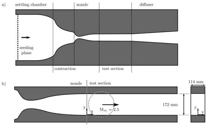
Experiments are performed in Supersonic Wind Tunnel No. 1 at Cambridge University Engineering Depart-ment. Figure 1a shows the infrastructure of the blow-down wind tunnel, which is driven by a high-pressure reservoir and exhausts to atmosphere. The stagnation conditions are measured in the settling chamber – for this study, the stagnation pressure is set at 308±1 kPa to avoid tunnel unstart and the operating stag-nation temperature is 285±5 K. The geometry consists of an 18:1 contraction with a round-to-rectangular transition, followed by a two-dimensional symmetric converging-diverging nozzle. The facility is capable of operating at Mach numbers between 0.7 and 3.5, depending on the installed nozzle configuration; for this study, the nominal freestream Mach number is fixed at M∞ = 2.5, which corresponds to a unit Reynolds
The rectangular working section of the tunnel has a width of 114 mm and a height of 172 mm. The coordinate system convention is shown in figure 1b. xrepresents the streamwise direction, as measured from the end of the nozzle; y indicates the floor-normal direction, with y = 0 mm set at the tunnel floor; z is the spanwise coordinate measured from the centre span, such that z =±57 mm correspond to the tunnel sidewalls.
The sidewalls of the working section take the form of removable doors, which are bolted onto the tunnel structure. The static pressure in the tunnel’s working section is below atmospheric pressure. Seal strips are used between the tunnel structure and sidewalls to prevent air from the surrounding environment being sucked into the tunnel due to the difference in pressures. This assists in maintaining good flow quality within the tunnel.
The inflow pressure uniformity is quantified by measuring the stagnation pressure distribution at the exit of the settling chamber, upstream of the nozzle. A Pitot rake is installed here, and the probes are connected to a differential pressure transducer NetScanner 9116. The measured pressure distribution is presented in figure 2. This shows a highly uniform flow over the tunnel cross-section, with a maximum variation in stagnation pressure across the entire inflow of 0.1%.
Within the working section, a z-type Schlieren system with a horizontal knife-edge enables visualisation of density gradients and allows flow features to be identified. Figure 3 shows that the flow in the tunnel is established; in addition, the boundary-layer on the tunnel floor, as well as weak Mach waves, are visible.
A final test of the working section flow in a routine wind-tunnel study would be to determine the thickness of the tunnel boundary-layers; this provides, for example, an estimate of the tunnel’s viscous aspect ratio. A measurement of the floor boundary-layer profile on the tunnel’s centreline is generally considered to be representative. To achieve this, the streamwise and floor-normal velocities,uandvrespectively, are measured using two-component LDV. The flow is seeded with paraffin using a vertical rake passing through the centre of the settling chamber (c.f. figure 1a). Previous measurements of particle lag through a normal shock have placed the seeding droplet diameter in the range 200–500 nm.5 Boundary-layer traverses are carried out with resolution ∆y ≈0.1 mm. The ellipsoidal probe volume spans 0.1 mm in the streamwise and vertical
nozzle test section 114 mm
y x M∞= 2.5 y z 172 mm settling chamber contraction nozzle test section diffuser a) b) seeding plane
Figure 1. Tunnel setup: a) Overall tunnel infrastructure. b) Detail of test section, showing dimensions and coordinate system. The dashed circle corresponds to a window in the tunnel wall providing optical access.
y / mm 0.9992 0.9998 0.9996 0.9994 p0/p0s −57 0 +57 z/ mm 0 216 162 108 54
Figure 2. Stagnation pressure measured by Pitot rake at exit of the settling chamber, upsteam of the nozzle. The Pitot probes are located in a square grid, at 20 mm intervals, betweenx=−50 and 50 mm and fromy= 8 to 208 mm.
Figure 3. Schlieren image for the empty tunnel with flow established.
0 25 20 15 10 5 y+ 100 101 102 103 104 u+ 0 5 10 15 0 100 200 300 400 500 600 a) b) measured data fitted profile log-law u+=y+
Musker Sun & Childs
u/ ms−1 y
/ mm
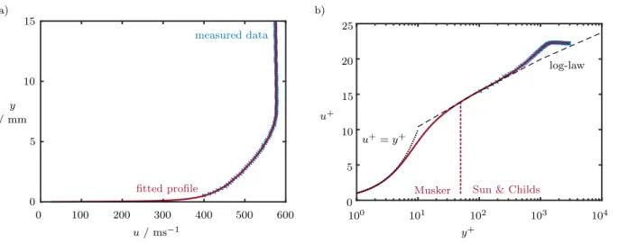
Figure 4. Boundary-layer LDV data and fitted profile in a) dimensional, and b) non-dimensional units. Mea-surements performed atx= 60 mm,z= 0 mm. In b), the data are presented in non-dimensional wall units,
u+= u uτ andy
+= yuτ
νw . The error bars are contained within the symbol size with ∆u= 5 ms
−1and ∆y= 0.1
mm
directions, and 2 mm in the spanwise direction.
The measured boundary-layer data is fitted to theoretical profiles (figure 4). A Sun & Childs (1973) fit,6 adapted to include a van Driest compressibility correction, is used for the outer layer; this combines a log-law of the wall region with a Coles wake function. The viscous sublayer is modelled using a Musker (1979) fit.7 These fitted profiles are then used to calculate characteristic boundary-layer integral parameters. This reduces errors caused by poor measurement resolution near the wall and therefore provides a more accurate estimate of integral boundary-layer parameters. The boundary-layer properties are determined in their incompressible forms, as these are less sensitive to variations in Mach number and require fewer assumptions to calculate from raw velocity data.
settling chamber contraction nozzle test section diffuser y x z
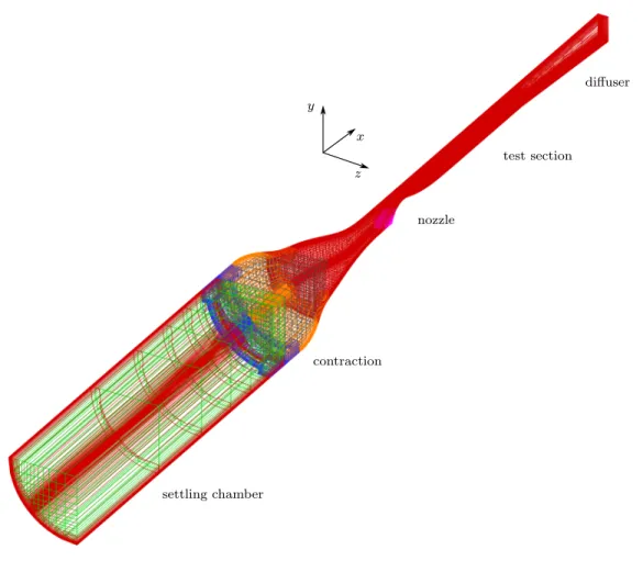
Figure 5. Representation of mesh used in computations to simulate physical tunnel.
has a shape factor of 1.34, indicating an equilibrium turbulent profile, and a thickness of 7.49 mm.
B. Computational method
Only one quarter of the tunnel is modelled since it is, in theory, top-bottom and left-right symmetric. The Chimera overset grid technique8 is used in order to create a smooth mesh in the round-to-square transition region and at the sharp corner upstream of the nozzle. The grid is created using the mesh generation software Pointwise.9 The final grid system contains 181.7M points across seven grids. To conduct a grid resolution study while maintaining the point distribution of the original grid, every other point is removed to create a medium grid (22.9M points), and every other point is removed from the medium grid to produce a coarse grid (2.9M points). A viscous wall spacing of 1.5×10⁻⁷m is used on the fine grid with a growth rate of 5%; this producesy+<1 at the first point from the wall for the coarse, medium, and fine grids. The coarse grid is shown in figure 5.
A nozzle boundary condition that fixes stagnation pressure and stagnation temperature at 308.0 kPa and 288.0 K respectively, as well as defining the flow angle to be perpendicular to the boundary, is used for the inflow. Meanwhile, an extrapolated boundary condition is used at the supersonic exit; this specifies the solution on the boundary plane to be equal to the solution one cell off the boundary’s surface. The walls are modelled with a no-slip condition and are isothermal at a room temperature of 291.15 K (18◦C). Care must be taken to avoid over defining the inflow boundary condition. Since neither stagnation pressure nor stagnation temperature profiles are uniform in a boundary-layer for fluids with non-unity P r,10 a no-slip wall cannot be used at the interface between the tunnel wall and the nozzle inflow boundary condition since this would impose a boundary-layer on the inflow plane. To overcome this, the walls that interface with the nozzle boundary condition are modelled as adiabatic slip-walls. An initial solution is generated using one-dimensional nozzle theory.
0 25 20 15 10 5 u+ 0 5 10 15 y+ 100 101 102 103 104 300 400 500 600 u/ ms−1 y / mm a) b) x= 60 mm fine medium coarse x= 70 mm x= 80 mm x= 90 mm y+ 100 101 102 103 104 300 400 500 600 u/ ms−1 y+ 100 101 102 103 104 300 400 500 600 u/ ms−1 y+ 100 101 102 103 104 300 400 500 600 u/ ms−1
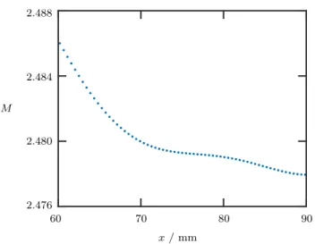
Figure 6. Calculated floor boundary-layer profiles for the coarse, medium and fine CFD solutions. These are calculated on the centre span atx= 60, 70, 80 and 90 mm, and are presented in both a) dimensional and b) wall units. 60 70 80 90 x/ mm M 2.476 2.488 2.484 2.480
x/ mm δ/ mm δi∗ / mm θi / mm Hi
60 7.72 0.91 0.70 1.304
70 7.76 0.91 0.70 1.302
80 7.86 0.93 0.71 1.301
90 8.00 0.94 0.72 1.301
Table 1. Incompressible boundary-layer parameters, computed by CFD along the tunnel centre span. These correspond to the profiles presented for the fine grid in figure 6.
The solver OVERFLOW 2.2l11is used to solve the RANS equations using the third-order accurate upwind finite difference HLLC scheme12 combined with the Koren limiter,13 and turbulence is modelled using the Spalart-Allmaras model.14, 15 The time integration uses an unfactored SSOR implicit solution algorithm.16 To accelerate convergence to a steady state, both grid sequencing and multi-grid are implemented. Grid sequencing involves computing an initial solution on a coarse grid, then successively finer grids. Meanwhile, multi-grid is a process in which, for every solution step, the solution vector is updated based on corrections calculated on a coarse grid; this has the effect of damping out high frequency errors in the fine grid solution. Figure 6 shows the centre span boundary-layers on the test section floor for the three grid levels. The three velocity profiles are coincident in both dimensional and wall coordinates, indicating that the centre span profiles have reached grid convergence. Boundary-layer parameters for the computed profiles are shown in table 1. The floor boundary-layer is approximately 8 mm thick and has a shape factor of 1.3, typical of an equilibrium turbulent profile. Figure 7 shows the tunnel centre span Mach number which varies from 2.486 to 2.478 in the test section; this corresponds to a variation of 0.3% and represents good flow uniformity.
III.
Flow characterisation tests for validation study
A key requirement of a validation study is to characterise the physical tunnel well enough for CFD to compute the true flow. Frameworks by which this might be consistently achieved4, 17–19place an emphasis on detailed measurements of the inflow conditions, the as-tested geometry and the tunnel boundary-layers. Whilst most scientific investigations need simply a verification that the flow quality is “good”, a validation study requires further tests to provide a quantitative characterisation of the flow.
A. Quantitative calibration data
As-installed Tunnel Geometry
The precise, as-installed, tunnel geometry is measured by securing a dial test indicator to a three component traverse, and scanning along the target surface. This is performed for both the tunnel floor and sidewall, so that the profile of these surfaces can be mapped to within 0.01 mm. An early measurement of the tunnel geometry is presented in figure 8a. The tunnel is designed with a linear divergence of the walls to provide boundary-layer relief; however, the measured geometry shows deviations of up to 0.3 mm (4% of a boundary-layer thickness) from this. Whilst these small variations do not impact the flow quality, the departures from the design geometry could affect the quantitative comparison of experimental data with computation. The observed “bumpiness” was attributed to warping of the wooden liner material, and grooves burned into the surface by the LDV laser; therefore the liners were replaced with aluminium equivalents.
Figure 8b shows the geometry with aluminium walls; the variations from the design geometry are now on the order of 0.05 mm, or 0.8% of a boundary-layer thickness. The tilt in the spanwise direction is 0.06±0.10◦; the surface can therefore be considered flat in this direction (within error due to the alignment accuracy of the measurement apparatus). Along with the CAD model, these measurements provide an accurate geometry for simulations, as well as the capability to perform a sensitivity analysis for deviations from the design configuration.
a) i. ii. b) i. ii. a) i. ii. b) i. −1.0 −0.5 0.0 +0.5 y /mm 0 50 100 150 200 250 x/ mm −1.0 −0.5 0.0 +0.5 y /mm 0 50 100 150 200 250 x/ mm −1.0 −0.5 0.0 +0.5 y /mm −57 0 z/ mm +57 +1.0 ii. −0.2 −0.1 0.0 +0.1 y /mm −57 0 z/ mm +57 +0.2
Figure 8. Measurement of tunnel floor geometry with a) wooden liners and b) aluminium liners. The mea-surements are performed i. in the streamwise direction at z= 0 mm, and ii) in the spanwise direction at
x= 0 mm. The error bars are contained within the symbol size with ∆y= 0.01 mm.
0 43 86 129 172 −100 −50 0 50 100 150 200 250 x/ mm y mm p/p0 0.054 0.070 0.066 0.062 0.058
Figure 9. Static pressure distribution measured using taps located in the tunnel sidewall. The red lines correspond to high-pressure areas; these take the form of oblique (solid) and vertical (dashed) regions.
0 5 10 15 a) x= 90 mm x= 80 mm x= 60 mm 300 600 u/ ms−1 450 300 600 u/ ms−1 450 300 600 u/ ms−1 450 300 600 u/ ms−1 450 y / mm b) 60 80 x/ mm 70 90 δi∗ / mm 0.8 1.0 1.2 c) 0 5 10 15 0 600 u/ ms−1 200 400 y/δ∗i x= 70 mm
Figure 10. a) Floor boundary-layer profiles measured using LDV. These are performed at different streamwise locations on the centre span. b) Variation in displacement thickness with streamwise direction. c) Collapse of profile shape whenyis non-dimensionalised by displacement thickness.
x/ mm δ/ mm δ∗ i / mm θi / mm Hi 60 7.49 0.97 0.73 1.341 70 7.59 1.03 0.74 1.351 80 7.70 1.05 0.76 1.356 90 7.71 1.05 0.78 1.354
Table 2. Incompressible boundary-layer parameters, measured along the tunnel centreline. These correspond to experimental profiles presented in figure 10a.
Sidewall Static Pressures
To quantify the strength of the weak waves identified in the schlieren image (figure 3), steady-state surface pressure measurements are performed using 0.3 mm diameter static pressure taps (error: ±1%).5 The taps are located across the tunnel sidewall, allowing the pressure distributions over the surface to be measured. Figure 9 shows that the wall static pressure varies by 4% throughout the working section. These deviations correspond to departures in free-stream Mach number of 0.02 from its mean value of 2.48. The oblique features in the plots correspond to weak waves generated from the tunnel floor and ceiling, whereas the vertical columns are due to spanwise-travelling waves produced by the sidewall.
Velocities in Working Section
In order to calibrate computational models, one set of boundary-layer profile data is not sufficient. The centre span floor boundary-layer is measured at several streamwise locations (figure 10a) to characterise its growth. The boundary-layer parameters corresponding to these profiles are tabulated in table 2. The profile shape is typical for a fully developed turbulent equilibrium boundary-layer, with an incompressible shape factor Hi ≈1.3. The growth of the boundary-layer with streamwise position is also evident. When normalised for boundary-layer thickness, as performed in figure 10c, there is a collapse of the profiles. The
constant profile shape in this region suggests that the waves identified in figure 9 are not strong enough to disturb the wall boundary-layers. In addition, measurements are performed on the boundary-layer away from the symmetry plane, and on the sidewalls (figure 11). The evaluated velocity distribution is used to characterise the flow field as completely as possible, enabling a more exhaustive calibration of computations.
B. Efforts to identify systematic errors
In the quantitative flow characterisation outlined above, random errors can be minimised by performing a greater number of relevant measurements. However, in order to use data for model calibration, it is essential to identify and account for any systematic errors; these bias the measured data and are generally not simple to detect or resolve. The identification of potential systematic errors is performed by implementing redundant tests, assessing the reliability of methods, and evaluating the repeatability of data.
Comparison Between Ldv and Pitot Tubes
The validity of LDV flow velocity data is tested through direct comparison with equivalent measurements using Pitot tubes. The Pitot probe experiments are conducted with no seeding rake (or seeding particles), and so this comparison also highlights any effect on the flow of the seeding apparatus.
The streamwise velocity, averaged over a circular region of diameter 0.3 mm, is also measured using Pitot tubes connected to a stepper-motor controlled traverse. To avoid position errors caused by constant probe bending under aerodynamic load, wall-normal positions are calibrated by the contact between the Pitot tube head and tunnel floor in the wind-on condition; this contact is detected electrically. It is possible to check that probe errors due to slow response time do not affect the data by comparing data from traverses performed in opposite directions (figure 12a) and at varying speeds (figure 12b). The former displays the effects of temporal lag, and allows the uncertainty in probe measurements to be estimated as ±3%. Meanwhile, Figure 12b shows that at speeds lower than 0.7 mm/s, theyposition is inaccurate due to the motor skipping steps, while it stalls at speeds faster than 1.5 mm/s. Thus, a suitable traverse speed of 1.2 mm/s is selected for this study.
An initial comparison of Pitot probe data with LDV, presented in figure 13a, shows reasonable agreement. However, there is a discrepancy in Mach number towards the outer edge of the flow. This comparison between methods is sufficient for scientific studies where, often, only the difference between measured profiles is of
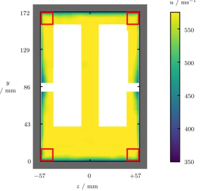
u/ ms−1 z/ mm 0 +57 −57 y / mm 0 43 86 129 172 550 500 350 450 400
Figure 11. Streamwise flow velocities measured across the tunnel cross-section atx= 120 mm. Corner regions, marked by red boxes, are excluded for calibration purposes.
b) a) 0.2 0.3 0.6 0.5 0.4 p02 /p0s 0 4 8 12 y/ mm 0.2 0.3 0.6 0.5 0.4 p02 /p0s 0 4 8 12 y/ mm upwards downwards 0.7 mm/s 1.0 mm/s 1.2 mm/s 1.5 mm/s
Figure 12. Pitot tube boundary-layer measurements carried out atx= 60 mm andz= 0 mm. These corre-spond to traverses performed a) both towards and away from the tunnel floor, and b) with varying traverse speed, conducted in the downwards direction.
y / mm 0 5 10 15 20 0 1 2 M 0.5 1.5 2.5 y / mm 0 5 10 15 20 0 4 12 t/ s 8 16 y / mm 0 5 10 15 20 0 1 2 M 0.5 1.5 2.5 a) b) c) LDV Pitot const. deflection from schlieren LDV Pitot (corrected)
Figure 13. a) Initial comparison of floor boundary-layer profiles measured at x= 120 mm and z= 0 mm between Pitot tube and LDV measurements. b) Probe position over course of traverse assuming constant deflection under aerodynamic load and measured from schlieren images. c) Comparison of the floor boundary-layer profile between Pitot tube and LDV measurements with corrected probe position.
350 400 450 600 u/ ms−1 y / mm 0 15 10 5 500 450 upwards downwards
Figure 14. Floor boundary-layer profiles measured using LDV at x= 120 mm and z= 0 mm, comparing velocity measurements between traverses performed in the upwards and downwards directions.
importance. However, errors of the magnitude seen here would hinder calibration of computational models. Rather than assuming constant probe deflection due to the wind-on condition, the position of the probe is more accurately determined using schlieren images of the tunnel. Figure 13b shows the assumed probe position and calibrated probe position over the course of a traverse; the deflection of the Pitot tube varies over the course of the run.
The boundary-layer profile with a recalibrated position is presented in figure 13c. This now demonstrates better agreement with the LDV profile, within intrinsic experimental error. Therefore the effect of seeding the flow is smaller than measurement resolution, and LDV data can now be used for model calibration with greater confidence. a) i. y / mm 0 5 10 15 20 37 42 47 52 57 z/ mm y / mm 0 5 10 15 20 37 42 47 52 57 z/ mm b) i. y / mm 0 5 10 15 20 37 42 47 52 57 z/ mm ii. u/ ms−1 350 550 500 450 400 ∆u/ ms−1 +20 −20 +10 0 −10 ∆u/u(%) +2.5 −2.5 −1.5 0 +1.5 ii. c) y / mm 0 5 10 15 M 0 2.5 z= 42 mm 0 2.5 z= 44 mm 0 2.5 z= 46 mm 0 2.5 z= 48 mm 0 2.5 z= 50 mm 0 2.5 z= 52 mm 0 2.5 z= 54 mm 0 2.5 z= 56 mm
Figure 15. Measurement of velocity distribution in corner region using a) i. vertical and ii. horizontal traverses. Red lines designate traverse locations. b) i. Difference between interpolated velocity distributions using both data sets, and ii. corresponding histogram of percentage velocity differences. c) Selected vertical boundary-layer profiles from a) i., showing comparison of velocities at intersection points with horizontal traverses.
Tests of Ldv Traverse
In order to identify systematic errors with the LDV-traverse measurement process, equivalent floor boundary-layer traverses were performed in both the upwards and downwards direction. A comparison between these measurements is presented in figure 14; the profiles collapse and calculated boundary-layer parameters show excellent agreement.
In addition, the flowfield across the tunnel span is typically measured by interpolating between several floor-normal traverses in they direction; an example of this is shown in figure 15a i. In order to ensure that these measurements are valid, traverses are also performed over the same region in the z direction (figure 4b ii). A visual representation of the interpolated flowfields appears to be identical in both cases. The difference between interpolated velocities (figure 15b) and the agreement of velocity at intersection points between the traverse sets (figure 15c) are evaluated. These both show a difference between interpolated velocity distributions of less than 10 ms−1(1.5% of freestream velocity).
These tests suggest that any systematic errors associated with the LDV-traverse system are no larger than the intrinsic experimental error associated with measurements.
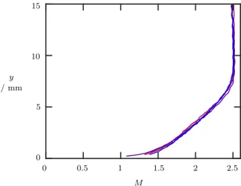
Tests of Repeatability
The wind tunnel is set up by installing liners within the tunnel structure. These liners are removed be-tween tunnel entries. Phenomenological investigations are able to gain useful information by comparing data obtained within the same tunnel entry; for validation studies, however, it is important to assess the repeata-bility between installations and quantify the resultant effect on flowfield variations. Figure 16 presents a floor boundary-layer traverse at the same location conducted during four separate tunnel installations several months apart. The excellent agreement between the profiles demonstrates good repeatability of the flowfield. More quantitative indications of the repeatability are the small variation in the freestream Mach number (2.48 to 2.51) and the narrow range of measured boundary-layer thicknesses (8.1 mm to 8.5 mm).
Tests of Symmetry
A common assumption of wind-tunnels with rectangular cross-sections is that, as per design, they are top-bottom and left-right symmetric. Whilst typical scientific studies are insensitive to subtle asymmetries in the flow, characterising these is an important feature of validation studies. The inability of LDV to measure the top half of the tunnel (due to seeding particle distribution and the tilt of laser optics) limits the ability to directly test top-bottom symmetry. As an alternative, the nozzle blocks and liners are swapped from the top to the bottom half of the tunnel, and vice versa; this permits identification of any top-bottom asymmetries downstream of the contraction.
To ensure that reversing the liners does not affect the flow itself, velocities at equivalent locations before and after the swap are compared. Due to the seeding particle distribution, this could only be performed for
0 0.5 1 2.5 M y / mm 0 15 10 5 1.5 2
Figure 16. Floor boundary-layer profiles measured using LDV at x= 120 mm and z= 0 mm, comparing velocity measurements between four different tunnel installations.
a) i. ii. b) i. ii. a) i. y / mm 86 96 −10 0 +10 z/ mm b) i. ii. u/ ms−1 550 590 580 570 560 ∆u/ ms−1 +20 −20 +10 0 −10 ∆u/u(%) +2.5 −2.5 −1.5 0 +1.5 ii. 76 y / mm 86 96 −10 0 +10 z/ mm 76 y / mm 86 96 −10 0 +10 z/ mm 76
Figure 17. Core flow in overlapping region atx= 120 mm a) i. before and ii. after nozzle blocks and liners have been top-bottom swapped. b) i. Difference between equivalent velocity measurements, and ii. histogram of percentage velocity differences.
a sub-region of the core flow. Figures 17a shows very similar (uniform) velocity distributions in this area before and after the swap. The difference between these distributions, given in figure 17b, shows that the velocities in equivalent locations in the core flow change by less than 0.7% on swapping the liners.
Figures 18a presents the floor boundary-layer before and after the swap is performed; these appear to be qualitatively very similar. The difference between the two profiles is plotted in figure 18b; this shows that equivalent velocities differ by at most 5 ms−1, or 0.8% of the freestream velocity.
In order to assess the left-right symmetry of the tunnel, all measurements are performed on both sides of the tunnel centreline. Figure 11, for example, presents the velocity field across the entire tunnel span. The difference between equivalent velocities in the left-right direction is shown in figure 19; departures from the case of left-right symmetry are no larger than 10 ms−1, or 1.6% of the freestream velocity.
Incidentally, these checks of left-right symmetry have been useful in identifying seal failures in the tunnel. The bolting mechanism of the tunnel doors is such that, in the case of a poorly sealed tunnel, air is not sucked into the working section symmetrically; seal failures can therefore be identified by checks of left-right symmetry. As an example, figure 20a presents an initial measurement of the floor boundary-layer across the span of the tunnel; it is clear that there is a very different flowfield between the left and right half of the tunnel. This is highlighted by large differences between individual boundary-layer traverses in equivalent locations (z=−52 mm and +52 mm), as shown in figure 20a ii. After replacing the wind tunnel seals, the flowfield appears to be left-right symmetric (figure 20b i) and equivalent boundary-layer traverses, shown in figure 20b ii, are approximately coincident. Thus this measurement can be used to identify leaks, which can often be difficult to identify but impact large areas of the flowfield. To avoid leaks reoccurring in the future, the seals are also inspected visually each time the tunnel doors are unbolted (at least every five wind tunnel runs).
Note that the equivalent velocities in both sets of symmetry test data are very similar but not identical. This is a feature of the “imperfect” physical tunnel; these differences can either be used to calibrate CFD or form an estimate of the error in these measurements.
−40 −20 0 20 z/ mm 40 ∆u/ ms−1 +20 −20 +10 0 −10 a) i. y / mm 0 5 10 15 u/ ms−1 350 550 500 450 400 ii. y / mm u/ ms−1 350 550 500 450 400 b) i. y / mm ∆u/u(%) +2.5 −2.5−1.5 0 +1.5 ii. −40 −20 0 20 z/ mm 40 −40 −20 0 20 z/ mm 40 0 5 10 15 0 5 10 15
Figure 18. Floor boundary-layer measured across tunnel span atx= 120 mm a) i. before and ii. after nozzle blocks and liners have been top-bottom swapped. b) i. Difference between velocity distributions, and ii. histogram of percentage velocity differences.
∆u/ ms−1 +20 −20 +10 0 −10 ∆u/u(%) +2.5 −2.5−1.5 0 +1.5 ii. 20 0 z/ mm 0 20 30 10 y / mm 40 57 i.
Figure 19. Difference between profiles in left- and right-hand halves of tunnel cross-section measurements at
C. Comparison between experiment and simulation
Comparison of Equivalent Quantities
An important aspect of calibrating a computational model is the comparison with experimental data. Dur-ing this process, it is important to treat measurements and computations in a similar fashion in order to accurately compare them. An example of this is the processing of sidewall static pressure measurements, shown in figures 21a and 21b. The computational solutions are first interpolated onto the experimental measurement locations in order to eliminate any perceived differences caused by the difference in spatial resolution.
The difference between the computational (figure 21b) and experimental (figure 21c) sidewall pressure distributions is plotted in figure 21d. The measured and computed static pressures agree to within about 3%. However, CFD generally under predicts the pressure, with the flow expanding to a lower pressure and a higher Mach number than the experiment. The top-left corner shows a higher pressure region that is just completing its expansion through the nozzle. The simulations appear to capture the weak waves generated by the tunnel floor and ceiling and show that these correspond to uncancelled waves from the nozzle. However, the computations do not seem to reproduce the waves produced by the tunnel sidewalls.
Computed boundary-layer profiles also need to be treated carefully when comparing with experimental velocities. LDV measurements are typically reported as point values, but they are measured as an average velocity of particles that pass through a finite probe volume created by intersecting laser beams. In order to assess how well the LDV measurements represent a point value of velocity, the CFD solution is interrogated in an analogous manner to the experimental measurement of the tunnel flow. An orthogonal mesh of dimensions 0.1×0.1×2.0 mm with a uniform spacing of 10−5 mm was created to represent the LDV volume; this is shown in figure 22. The “long” grid dimension of 2.0 mm is aligned with the span of the tunnel.
A boundary-layer profile was extracted from the computational simulation. The representative LDV volume was centred at a point on the extracted profile, and the volume CFD solution was interpolated onto the LDV volume grid; the velocity values in this region were then averaged. By averaging uniformly across the simulated LDV volume, a conservative estimate is obtained for the averaging effect in real LDV measurements where i) the probe volume is ellipsoidal, and ii) the data is biased towards particles passing through the centre of this region.
y / mm u/ ms−1 350 550 500 450 400 b) i. z/ mm z/ mm 0 5 10 15 0 5 10 15 u/ ms−1 350 550 500 450 400 a) i. y / mm −57 −40 −20 0 20 40 57 ii. 0 5 10 15 y / mm 400 u/ ms−1 600 500 ii. 0 5 10 15 y / mm 400 u/ ms−1 600 500 −57 −40 −20 0 20 40 57
Figure 20. Floor boundary-layer atx= 120 mm with the tunnel a) poorly sealed and b) correctly sealed. Figure shows i. velocity distribution across tunnel span and ii. individual boundary-layer profiles atz=−52 mm and
p/p0 0.053 0.065 0.062 0.059 0.056 x/ mm y / mm 86 161 111 136 −100 −50 0 50 100 150 200 250 p/p0 0.053 0.065 0.062 0.059 0.056 x/ mm y / mm 86 161 111 136 −100 −50 0 50 100 150 200 250 p/p0 0.053 0.065 0.062 0.059 0.056 x/ mm y / mm 86 161 111 136 −100 −50 0 50 100 150 200 250 ∆p/p0 −0.0070 +0.0070 +0.0035 0.0000 −0.0035 x/ mm y / mm 86 161 111 136 −100 −50 0 50 100 150 200 250 a) b) c) d)
Figure 21. Computed static pressure on the tunnel sidewall a) prior to and b) after interpolating onto experimental measurement grid. c) Experimentally measured sidewall static pressure (c.f. figure 9). d) The difference between the two static pressure distributions. The red lines correspond to high-pressure areas; these take the form of oblique (solid) and vertical (dashed) regions.
y x
z
0 5 10 y / mm 0 200 400 600 u/ ms−1 CFD profile volume-averaged CFD 0 5 error (%) error y−ywall (%) / mm 0.1 0.35 0.5 0.16 1.0 0.62 −57 z / mm 0 200 400 600 u/ ms−1 CFD profile volume-averaged CFD 0 5 error (%) error z−zwall (%) / mm 0.1 4.89 0.5 2.13 1.0 1.54 −52 −47 a) b) 4 3 2 1 4 3 2 1
Figure 23. Comparison of CFD streamwise velocities extracted from the solution and CFD values interpolated onto a representative LDV measurement volume, then averaged for a) the floor boundary-layer (x= 60 mm,
z= 0 mm) and b) the sidewall boundary-layer (x= 60 mm,y= 15 mm).
Figure 23a shows the results for a floor boundary-layer profile on the tunnel centreline, while figure 23b shows the equivalent results for the sidewall boundary-layer. The floor boundary-layer does not show any noticeable difference between the extracted and averaged profiles above about 0.1mm from the wall. This is however not true for the sidewall boundary-layer. Here, the velocity values normal to the wall are averaged over 2.0 mm rather than 0.1 mm; thus, the averaging region now forms a significant proportion of the boundary-layer thickness. This causes averaged velocities within 2 mm of the wall to show a discrepancy from the point values, and sidewall reflections prevent any measurements within 1 mm of the wall. More importantly, however, the simulations enable a confident estimate of the velocity error due to the finite probe volume – this error cannot be extracted from experimental data alone.
Calibration Process
In order to determine the run conditions for the three-dimensional grids, preliminary solutions were computed on a two-dimensional grid representing the centre span of the tunnel; these are much cheaper to compute. The first simulations were conducted with adiabatic walls and given inflow stagnation conditions of 308 kPa and 285 K. The boundary-layer profiles using Spalart-Allmaras,14, 15 Menter SST,20, 21and Wilcox k-ω22, 23 turbulence models were compared (figure 24a). While the difference between the turbulence models is minimal, the SA model matched the LDV measurements best.
Figure 24a also shows that the freestream velocity at x= 60 mm is not accurately reproduced by the CFD. This is solved by tuning the specified inflow stagnation temperature to 288 K in order to match the measured freestream velocity, as shown in figure 24b. Note that the new stagnation temperature falls within the reported uncertainty in the measured stagnation temperature (285±5 K). Next, the effect of wall temperature is investigated. When conducting measurements, the run time of the tunnel is short enough that the tunnel walls are assumed to be isothermal. A wall temperature of 291.15 K (18◦C) is chosen to represent the room temperature in which the test section resides. A comparison between boundary-layer profiles using adiabatic walls and isothermal walls at 291.15 K is shown in figure 24c. The effect of wall temperature on the velocity profile is negligible but, since isothermal walls form a more accurate representation of the actual wind tunnel, the three-dimensional simulations are also modelled by isothermal walls.
Comparison of boundary-layers
A comparison between computational and experimental floor boundary-layer profiles is presented in figure 25; the boundary-layer parameters obtained from these profiles are given in tables 1 and 2. There is good agreement in the freestream velocities between the simulations and the measurements, but the profiles differ in the lower regions of the boundary-layer. These discrepancies are greater than the associated uncertainties,
u+ y / mm 0 25 20 15 10 5 0 5 10 15 y+ 100 101 102 103 104 300 400 500 600 u/ ms−1 Spalart-Allmaras Menter SST experiment (LDV) y+ 100 101 102 103 104 300 400 500 600 u/ ms−1 y+ 100 101 102 103 104 300 400 500 600 u/ ms−1 a) b) c) T0= 288 K T0= 285 K isothermal (18◦C) adiabatic Wilcoxk−ω experiment (LDV) experiment (LDV)
Figure 24. Computed floor boundary-layer profiles on the tunnel centre span atx= 60 mm over the calibra-tion process, showing the effect of a) turbulence model, b) stagnacalibra-tion temperature, and c) wall temperature condition. 0 25 20 15 10 5 u+ 0 5 10 15 y+ 100 101 102 103 104 300 400 500 600 u/ ms−1 y / mm a) b) x= 60 mm computation experiment (LDV) x= 70 mm x= 80 mm x= 90 mm y+ 100 101 102 103 104 300 400 500 600 u/ ms−1 y+ 100 101 102 103 104 300 400 500 600 u/ ms−1 y+ 100 101 102 103 104 300 400 500 600 u/ ms−1
Figure 25. Comparison between computational and experimental floor boundary-layer profiles. CFD profiles are calculated using the fine mesh. The profiles are shown forx= 60, 70, 80 and 90 mm, and are presented in both a) dimensional and b) wall units.
settling chamber corner rake from seeder contraction b) c) d) x= 60mm a) y x z y z y / mm 0 15 −57 −40 −20 0 20 40 57 x/ mm data rate / kHz 0 20 10 e) y / mm 0 15 −57 −40 −20 0 20 40 57 x/ mm data rate / kHz 0 20 10
Figure 26. a) Seeding rates across the floor boundary-layer when using the existing seeding rake. b) Schematic cross-sectional view of corner seeding system, located in the tunnel’s settling chamber. Seeding particles are introduced to the flow from the corner rakes. c) Simulated streamlines traced upstream into the settling chamber. d) Isometric view of simulated corner flow streamlines illustrating the ‘seeding plane’ in the corner region of the working section. e) Seeding rates across the floor boundary-layer when using the corner seeding system.
and thus suggest a systematic problem with the simulations. The differences in boundary-layer profile therefore warrant further investigation.
Presentation of Data
In science discovery investigations, data is often presented in such a way as to highlight features of interest, perhaps at the expense of other aspects of the flow. Examples of this include the choice of colour map for a contour plot or the knife-edge orientation for schlieren techniques. The presentation of, and comparison between, data sets in a validation experiment needs to be more objective than this, however. The colour map for data presentation is chosen to be perceptually uniform with appropriate ranges to accurately represent the information. Schlieren visualisations for the flow with various knife-edge orientations, in combination with a shadowgraph, are conducted to obtain a complete picture of the flowfield.
D. Benefits of close experimental-computational collaboration
In many validation projects, computations aim to replicate previous experimental measurements. However, the wind tunnel and numerical tests for this study are performed and more, importantly, designed simulta-neously. Computations, before they are calibrated or even converged, can still provide useful information to experimentalists, despite perhaps not accurately capturing all aspects of the flow. The considerable benefits
of this close collaboration are highlighted in several aspects of the work, as outlined below.
Corner Seeding and Sidewall Boundary-Layers
The primary area of interest to this study is centred on the corners of the wind tunnel channel. Originally, these regions were not well seeded (figure 26a) – data rates in excess of 10 kHz are required to obtain validation quality LDV measurements. In order to probe this region, modifications to the seeding system were required to introduce seeding particles into the corner region. The corner seeding system, located upstream of the contraction in the settling chamber, is sketched in figure 26b. Computations of the tunnel were used to determine the optimum rake location. Streamlines were traced upstream from the corner region in the working section to the relevant plane in the settling chamber (figures 26c and 26d). Placing the rake at this location ensures that seeding particles introduced to the flow pass through the corner region in the working section. The seeding rates measured after the installation of the new rake (figure 26e) demonstrate that the modification was successful, and so validation-quality reference data can be collected in the corner regions. a) i. u/ ms −1 z/ mm 0 +57 −57 y / mm 0 43 86 129 172 550 500 350 450 400 ii. z/ mm 0 +57 −57 y / mm 0 43 86 129 172 20 -20 10 0 -10 v/ ms−1 b) i. u/ ms −1 z/ mm 0 +57 −57 y / mm 0 43 86 129 172 550 500 350 450 400 ii. z/ mm 0 +57 −57 y / mm 0 43 86 129 172 20 -20 10 0 -10 v/ ms−1
Figure 27. a) Experimental and b) computational measurements of the velocities across the tunnel cross-section. The i. streamwise and ii. vertical velocities are both presented, and show evidence of secondary flows within the sidewall boundary-layers.
In addition, these seeding rakes introduce seeding into a region that enables sidewall boundary-layer measurements to be performed. The sidewall boundary-layer data (figure 11) forms an important part of simulation calibration but also presents useful physical insight. The measurements in this region reveal the presence of vertical velocities within the sidewall boundary-layers (figure 27a). As explained in reference 24, these secondary flows are a previously unknown feature of rectangular supersonic wind tunnels, and they can have a significant effect on the flow development in the corner regions.
Whilst the experiments alone do identify the sidewall secondary flows, the data in this region is limited and has relatively large uncertainties, as shown in figure 23. Therefore, the fact that even preliminary simulations capture equivalent behaviour in the sidewall boundary-layers (figure 27b) confirms that these effects are indeed physical rather than being an artefact of the experimental method.
This is a salient example of the synergetic benefits of close collaboration between those performing computations and experiments. Computations benefit from sidewall calibration information and higher quality validation data in the corners. Meanwhile, the wind tunnel infrastructure improved as a result of informed guidance on the optimum seeding rake location, enabling experimental data to be collected in previously inaccessible regions.
Separation Upstream of Nozzle
A schlieren image of the flow was presented in figure 3. When the exposure time is reduced from 0.1 ms to 1.1µs, turbulent eddies become visible (figure 28a). Two streamwise flow features above and below the tunnel centre height can also be resolved, but it is not clear what these are or where they originate.
From simulations of the tunnel, these features can be associated with vortices present along the tunnel sidewalls (Figure 28b). These appear to originate from a region immediately upstream of the nozzle; here, the subsonic flow separates when it encounters a forward-facing step. Oil flow visualisation performed in this region to confirm the presence of such a separation is shown in figure 28c. The size and shape of the separation is in agreement with the computations.
In order to remove the vortices from the test section flow, the geometry upstream of the nozzle is redesigned by filleting the forward-facing step. Numerical and experimental tests are currently in progress to determine the effect of the geometry change on the separation and, in turn, vortices along the test section sidewalls.
Note that the merits of close experimental-computational collaboration are not limited to flow character-isation and model calibration. During validation, experimental data in the corner boundary-layers will enable improvement of numerical methods. Moreover, the computations provide information inaccessible from experiment alone – in particular, the ability to identify and track streamwise vortices in the corner boundary-layer will enhance physical insight of this flowfield.
b) c) a)
y x z
Figure 28. a) Schlieren image with short exposure time, with unidentified streamwise features highlighted. b) RANS simulation showing vortices along the tunnel sidewalls. These originate from a separation region (yellow) upstream of the nozzle. c) Oil flow visualisation in region upstream of the nozzle; separation region is highlighted in yellow.
IV.
Conclusions
Validation studies in high-speed aerodynamics are becoming increasingly relevant to investigations of com-plex flow problems. This paper presents the characterisation process for a joint experimental-computational investigation focused on the flow in the streamwise corner of a channel with freestream Mach number 2.5. The usual checks of good flow quality for a typical phenomenological study show that the inflow stagnation pressure is uniform to within 1%, that the flow is established and that the tunnel wall boundary-layers are about 7 mm thick. However, further quantitative calibration data is required to set up accurate simula-tions of the physical flow. This involves careful measurements of the as-installed tunnel geometry, sidewall static pressure distribution and flow velocities across the tunnel cross-section, whilst quantitatively testing assumptions about the experimental methods and setup.
This more detailed investigation confirmed that the measurement techniques are reliable (within stated experimental error), but has also revealed some interesting findings about the flow within the tunnel:
• the original wooden tunnel floor had inherent variations on the order of 4% of a boundary-layer thick-ness, and replacing these with alumninium reduced variations by a factor of five;
• weak Mach waves generated by the tunnel floor and sidewall can be identified – initial computations capture the former but not the latter;
• these weak waves cause Mach number variations of less than 0.9% and do not affect the profile shape of the floor boundary-layer;
• Pitot probe measurements are susceptible to variable deflection over the course of a run – when this is accounted for, the boundary-layer profile matches LDV data, showing that the seeding apparatus does not influence the flow;
• between tunnel installations many months apart, the freestream Mach number varies by 1.2% and the boundary-layer thickness varies by 5%;
• the velocities in the tunnel are top-bottom and left-right symmetric to within 2%, and any deviations from the left-right symmetry of the tunnel are good indicators of sealing problems – this is a particularly important test, as leakage can be difficult to identify.
There are also strong synergetic benefits due to the close collaboration between those conducting experiments and computations. This combined effort is a crucial aspect of the design, execution and analysis of a validation study, and also has served to:
• more accurately assess the error due to averaging LDV data over a finite probe volume for floor (1% error at 0.12 mm from wall) and sidewall (1% error at 1.54 mm from wall) boundary-layer measurements;
• install a corner seeding system into the setup, configured using the informed guidance of computations;
• obtain sidewall boundary-layer calibration data that enables identification of important secondary flows in these regions;
• identify a physical separation region upstream of the nozzle associated with streamwise vortices along the tunnel sidewall;
In conclusion, with validation studies becoming increasingly relevant and significant in tackling complex flow problems, it is essential to calibrate relevant computational models with accurate characterisation data. This takes the form of quantitative measures of the flow whilst taking care to identify and eliminate any systematic errors. The characterisation process and, in particular, close experimental-computational collaboration yields strong benefits in terms of better understanding the physical characteristics of the tunnel flow.
Acknowledgements
The authors would like to thank David Martin, Anthony Luckett and Ciaran Costello for operating the blowdown wind tunnel. The wind tunnel is part of the UK National Wind Tunnel Facility (NWTF) and their support is gratefully acknowledged. The research leading to these results has received funding from the Air Force Research Laboratory.
References
1J. Benek. Corner flows: motivation & objectives. Comments made at the10th Annual Shock Wave/Boundary Layer Interaction (SWBLI) Technical Interchange Meeting, 2017.
2N. Titchener and H. Babinsky. Shock wave/boundary-layer interaction control using a combination of vortex generators
and bleed. AIAA Journal, 51(5):1221–1233, 2013.
3H. Babinsky, J. Oorebeek, and T. Cottingham. Corner effects in reflecting oblique shock-wave/boundary-layer
interac-tions. In51st AIAA Aerospace Sciences Meeting, 2013-0859.
4D.P. Aeschliman and W.L. Oberkampf. Experimental methodology for computational fluid dynamics code validation. AIAA Journal, 36(5):733–741, 1998.
5S.P. Colliss, H. Babinsky, K. N¨ubler, and T. Lutz. Vortical structures on three-dimensional shock control bumps. AIAA Journal, pages 2338–2350, 2016.
6C.C. Sun and M.E. Childs. A modified wall wake velocity profile for turbulent compressible boundary layers.Journal of Aircraft, 10(6):381–383, 1973.
7A.J. Musker. Explicit expression for the smooth wall velocity distribution in a turbulent boundary layer.AIAA Journal,
17(6):655–657, 1979.
8J. Benek, J. Steger, and F.C. Dougherty. A flexible grid embedding technique with application to the Euler equations.
In6th Computational Fluid Dynamics Conference Danvers, 1983-1944.
9Pointwise Version 18.0R4. Pointwise Inc., Fort Worth, TX, 2017.
10E.R. Van Driest. Turbulent boundary layer in compressible fluids. Journal of the Aeronautical Sciences, 18(3):145–160,
1951.
11P.G. Buning, D.C. Jespersen, T.H. Pulliam, W.M. Chan, J.P. Slotnick, S.E. Krist, and K.J. Renze. Overflow user’s
manual. NASA Langley Research Center, Hampton, VA, 2002.
12E.F. Toro, M. Spruce, and W. Speares. Restoration of the contact surface in the HLL-Riemann solver. Shock Waves,
4(1):25–34, 1994.
13B. Koren. Upwind schemes, multigrid and defect correction for the steady Navier-Stokes equations. In11th International Conference on Numerical Methods in Fluid Dynamics, pages 344–348. Springer, 1989.
14P. Spalart and S. Allmaras. A one-equation turbulence model for aerodynamic flows. In30th Aerospace Sciences Meeting and Exhibit, 1992-0439.
15S.R. Allmaras and F.T. Johnson. Modifications and clarifications for the implementation of the Spalart-Allmaras
turbu-lence model. InSeventh International Conference on Computational Fluid Dynamics, ICCFD7-1902, 2012.
16R. Tramel and R. Nichols. A highly efficient numerical method for overset-mesh moving-body problems. In13th Com-putational Fluid Dynamics Conference, 1997-2040.
17W.L. Oberkampf and C.J. Roy. Verification and validation in scientific computing. Cambridge University Press, 2010. 18P.J. Roache. Fundamentals of verification and validation. Hermosa Publishers, 2009.
19C.J. Roy and W.L. Oberkampf. A comprehensive framework for verification, validation, and uncertainty quantification
in scientific computing.Computer methods in applied mechanics and engineering, 200(25-28):2131–2144, 2011.
20F. Menter and C. Rumsey. Assessment of two-equation turbulence models for transonic flows. InFluid Dynamics Conference, page 2343, 1994.
21F.R. Menter, M. Kuntz, and R. Langtry. Ten years of industrial experience with the SST turbulence model.Turbulence, Heat and Mass Transfer, 4(1):625–632, 2003.
22D.C. Wilcox. Reassessment of the scale-determining equation for advanced turbulence models. AIAA Journal,
26(11):1299–1310, 1988.
23D.C. Wilcox. Turbulence Modeling for CFD. DCW Industries, Inc., 3rd edition, 2006.
24K. Sabnis, D. Galbraith, H. Babinsky, and J. Benek. The influence of nozzle geometry on corner flows in supersonic wind