This PDF is a selection from an out-of-print volume from the National Bureau
of Economic Research
Volume Title: Essays on Interest Rates, Vol. 2
Volume Author/Editor: Jack M. Guttentag, ed.
Volume Publisher: NBER
Volume ISBN: 0-87014-224-0
Volume URL: http://www.nber.org/books/gutt71-2
Publication Date: 1971
Chapter Title: The Geographic Structure of Residential Mortgage Yields
Chapter Author: E. Bruce Fredrikson
Chapter URL: http://www.nber.org/chapters/c4001
Chapter pages in book: (p. 187 - 280)
4
The
Geographic Structure of
Residential Mortgage
Yields
E. Bruce Fredrikson
INTRODUCflON: SCOPE AND
FOCUS
This paper reports some results of an exploratory study of the influence
of property location on yields of conventional, residential mortgage
loans. It provides new benchmark data on comparative average
mort-gage yields and contract terms for regions, states, and metropolitan
areas in 1963; loan originations by five types of lenders for three
cate-gories of loan purpose are included in the sample data provided by
the Federal Home Loan Bank Board.
Some of the questions dealt with here are: Is property location a
mortgage yield determinant? What is the absolute level of differentials
between average mortgage interest rates in various regions of the
United States? How do these interregional differentials compare in
magnitude to those that may arise within various geographical regions—
for example, between two eastern metropolitan areas? Since aggregate
data include three categories of loan purpose, we may ask whether loan
purpose affects the size of differentials. Because of the diverse
insti-tutional structure and lending patterns of the several types of financial
intermediary, it
is of interest to inquire whether the regional pattern
of mortgage yields is generally similar for each of the five lender groups.
Finally, we study the effect of variations in contract terms on
corn-NOTE: I am deeply indebted to Jack Guttentag for his continued guidance
during this project.
188
Essays on Interest Rates
parative mortgage yield differentials. With the data at hand we are
able to measure yield differentials in the raw data and, in addition, to
take account of differences in key contract terms, obtaining thereby a
second estimate of the yield differential between two areas. Inspection
of the two sets of differentials provides a basis for determining whether
comparisons of simple average yields in different sections of the country
are valid, or whether, in contrast, geographic differences in contract
terms that affect yield are so large that they require a
statistical
correction. Because unadjusted national figures
are compiled and
distributed monthly by the Federal Home Loan Bank Board, and
presumably influence policy decisions at various levels of government,
interest in this question transcends the academic.
The Data
The data underlying the statistical results are unique in both
geo-graphic scope and detail; thus, a brief description is appropriate at this
point. Since December 1962, the Federal I-Tome Loan Bank Board
(FHLBB) has been compiling records of individual,
conventional
mortgage commitments on one-family, nonfarm homes on a sample
basis from lenders located throughout the United States. Roughly 14,000
mortgage transactions are reported monthly by a sample of lenders that
numbered approximately 3,000 during 1963. The magnetic tape record
for each loan includes the date, the amount of the loan, the value
or purchase price of the property, the maturity, the contract interest
rate, fees and charges, the type of lender, the loan purpose, and coded
location of both property and lender by Standard Metropolitan
Statis-tical Area (SMSA) or non-SMSA, state, Home Loan Bank District
(11 during the period of this study), census division (9), and region
(4). Effective interest rates were computed for this study on the
assumption that the unamortized principal is prepaid after one half of
the original maturity has expired.1 The weight used in all calculations
is the number of loans in the area under study rather than the dollar
amount of the loan.
The loans included in the present study represent commitments made
by selected lenders during the eight-month period of May—December
'For a discussion of alternative methods of computing effective rate, see Jack
M. Guttentag and Morris Beck, Mortgage Interest Rates Since 1951, New York,
NBER, 1970, Chapter 5.
1963,
inclusive, a period of relative yield stability in the mortgage
market. Nearly 110,000 loans are included in this sample. Of these,
46 per cent were made on properties located in 18 large SMSAs.2
Much of the analysis in this paper, including all of the regression runs,
is based on the data for these 18 SMSAs.
Mortgages examined during this study are distinguished according
to the loan purpose or the type of property being mortgaged. The "new
construction" category represents permanent building loans for
indi-viduals and homebuilders who do not utilize interim financing. The
"newly built" category refers to loans for the purchase of a newly
constructed (never occupied) home from a builder. The "previously
occupied" category includes loans for the purchase of existing houses.
The composition of the sample, by both loan purpose and lender
type, is presented below (all figures are a percentage of the total):
Previously
Newly
New
Occupied
Built
Construction Total
Life insurance companies
1.2
1.9
1.34.4
Mortgage companies
1.31.7
0.8
3.8
Savings and loan associations 40.5
14.2
14.3
69.0
Mutual savings banks
6.1
2.3
1.19.5
Commercial banks
9.6
1.7
2.1
13.4
Total
58.7
21.819.6
100.0
Et is obvious that loans by savings and loan associations, representing
more than two-thirds of the sample, dominate the data. Among types
of loan purpose, the total sample includes comparable weighting for
the newly built and new construction categories, while nearly 60 per
cent of the loans recorded represent mortgages issued for the purchase
of previously occupied homes. Because of the unequal weights accorded
the different categories of loan purpose and lender type, mean
statis-tics are presented, where available, for each group separately. In many
cases, mean data for each of the 15 combinations of lender type and
loan purpose are also presented.
When national or regional data are the subject of the analysis, the
number of observations in each cell generally ranges from a hundred
to several thousand. However, when the geographic area of interest
is the state or standard metropolitan area, the number of observations
2The
Home Loan Bank Board issues a monthly time series of average interest
190
Essays on Interest Rates
recorded for a given property and lender type may be small or even
zero. In particular, the regional concentration of mortgage companies
and mutual savings banks gives rise to many blank cells. Additionally,
even where all lender types are represented, the statistical significance
of some results may be limited by possible deficiencies in the original
sample and by nonuniform response rates by institutions included in
the survey group. Generally, the savings and loan associations, which
are directly regulated by the Federal Home Loan Bank Board, and the
mutual savings banks have had the highest response rate.
The loans analyzed in this paper are loans to original borrowers
involving the creation of a new mortgage instrument. No information
regarding the ultimate disposition of the loans is available. It may be
assumed, however, that virtually
all mortgage company loans were
originated for sale to ultimate lenders, principally life insurance
com-panies and mutual savings banks. Some commercial bank loans also
represent temporary commitments.
All of the loans in the FHLBB's sample were scheduled to be fully
amortized over the mortgage term, which was limited to maturities of
between five and forty years, inclusive. The five-year minimum term
was imposed principally to exclude construction loans by builders who
had not arranged for permanent owner financing.3
Method of Analysis
Two methods of analysis are used in this paper to measure yield
differentials. First, average yields in different areas are simply
com-pared. Because the records are coded by both region and metropolitan
area, it is possible to determine the approximate magnitude of both
inter- and intraregional yield differentials by examining mean rates
for various geographic subsets of the total sample. Further refinement
is made possible by classifying loans by either loan purpose or lender
type, or both. This procedure does not, however, fully utilize the
available data. Information on yield determinants such as the
loan-value ratio cannot be employed effectively by comparing averages.
Before
any calculations were made for this study, all observations were
sub-jected to a screening program, designed to eliminate apparently erroneous records
on the tapes, which limited the acceptable terms as follows: loan-value ratio, less
than 1.00 and greater than .06;
principalamount, $1,000 to $99,999; purchase
price, less than $100,000; contract interest rate, 3.00 to 9.99 per cent; fees and
charges, less than 6.0 per cent.
The second statistical method is multiple regression analysis, with
either effective interest rate or contract rate as the dependent variable.
From the entire sample, a subset representing 50,000 loans on
proper-ties in 18 principal SMSAs was drawn. In regressions covering all
50,000 loans, both lender type and loan purpose were held constant
with dummy variables in order to remove their specific effects. Then
17 dummy variables representing the SMSAs were introduced. The
resulting b-coefficients for the individual SMSAs provide an indication
of the differentials in mortgage interest rates between the metropolitan
areas included in the regression on loans standardized for loan purpose
and lender type. Three risk variables—purchase price, loan-value ratio,
and maturity—were then introduced in the regression and their impact
on yield differentials between metropolitan areas was assessed.
Sepa-rate regressions were run for each of the different lender type and loan
purpose groups.
The area differentials calculated from the regressions, while allowing
for the influence of some important yield determinants that are
corre-lated with area, may be influenced by others for which no allowance
could be made. These include the socioeconomic characteristics of the
neighborhood or broader area, which may be deteriorating or
develop-ing, integrated or segregated, residential or semicommercial. Transaction
characteristics that may be correlated with both yield and area include
the borrower's present and expected income and wealth, his age and
family size, and (on previously occupied homes) the age of the
property. Despite these shortcomings, the data presented in this paper
remain the most comprehensive available, or likely to be available,
for examining yield differentials on residential mortgages.
PROPERTY LOCATION AS A YIELD DETERMINANT
The multiple regression procedure permits a statistical determination
of the importance of property location as a mortgage yield
deter-minant. After the lender type and loan purpose had been introduced
into the regression, explained variance, as represented by the coefficient
of multiple determination (R2), was .3303. With the subsequent
intro-duction of the 17 property location dummy variables, R2 rose to .5124,
indicating that over 18 per cent of variance was explained by the
metro-politan area variables after both lender and property type were taken
192
Essays on Interest Rates
to property location in fact derived from differences in contract terms,
additional regressions in which the three risk variables were introduced
after the loan purpose and lender type variables and before the SMSA
variables were run. In this regression the introduction of property
location increased explained variation of effective yields by 21 per
cent, again indicating clearly the significance of the SMSA variables.
When the same regression format was employed on individual lender
type and loan purpose groups, similar results were obtained. After
lender type and contract terms were held constant, the increase in R2
on the loan purpose runs ranged from 17 per cent on newly built homes
to 26 per cent on loans for new construction.
Regressions covering the lender type series showed wide differences
in the significance of property location as a determinant of effective
interest rate. Contributions to explained variance, after holding
con-tract terms and loan purpose constant, ranged from 14 per cent for
life insurance company loans to 41 per cent for the mutual savings
bank sample. The complete tabulation (in per cent) of the contribution
of property location after the inclusion of lender type and loan purpose,
both before and after the inclusion of the three risk variables, appears
in the table below.
Increase in R2 Resulting From Introduction
of Property Location Variables
Into Effective Interest Rate Regressions
Before Risk
After Risk
Variables
Variables
All loans
18 21New construction
26
26
Newly built
18 17Previously occupied
20
24
Life insurance companies
1514
Mortgage companies
32
23
Savings and loans
3137
Mutual savings banks
46
41
Commercial banks
26
23
A tabulation of R2 and the standard error after each step for both
contract rate and effective rate regressions appear in Appendix Tables
4-AS and 4-A6. The location coefficients appear in Tables 4-A12 and
STRUCTURE OF INTERREGIONAL DIFFERENTIALS
Prior Research
Several previous researchers, using much less comprehensive data,
examined the broad structure of the national mortgage market and
drew tentative conclusions regarding the general nature of regional
differentials.
J. E. Morton's analysis of loans outstanding in 1947 provides the
following conclusions of interest, which are generally confirmed by
the present study: (1) Interest rates on nonfarm mortgage loans are
highest in the West and lowest in the North, with rates on Southern
properties falling in between. (2) Differences between rates charged
by various lender types are apparently greatest in the West and
South, as compared with the North. (3) Rates on loans by life
insur-ance companies showed less regional variation than those on
commer-cial bank loans.,4
Morton's data differ from those included in the present study in two
important respects.
First, Morton's data reflect loans outstanding,
rather than the commitment data underlying this, study. Loans
out-standing reflect net acquisitions over a period of years so that regional
yield differentials are influenced by dissimilarities in the time pattern
of acquisitions by different institutions in different areas.5 (The next
two studies referred to below also employ data on outstanding loans.)
Second, Morton's data only cover broad regions, while the data below
cover states and metropolitan areas as well.
Grebler, Blank, and Winnick considered the regional structure of
residential mortgage rates in historical perspective. Their conclusion
that interregional rate differentials have diminished since the late
nine-teenth century is based upon Table 4-1 (updated here with data from
the 1960 Census of Residential Housing) •6 In
1890 the interest rate on
urban mortgages was nearly 4 or 5 percentage points higher in some
sections of the country than in other sections because of the localization
1. E. Morton, Urban Mortgage Lending: Comparative Markets and
Experi-ence, Princeton, Princeton University Press for NBER, 1956, pp. 82—83.
For a discussion of the timing aspects of mortgage yield series, see
Gutten-tag and Beck, op. cit.
Leo Grebler, David M. Blank, and Louis Winnick, Capital Formation in
Residential Real Estate: Trends and Prospects, Princeton, Princeton University
Press for NBER, 1956, Chapter 15.
TABLE 4-1. Average Interest Rate on Residential Mortgages Outstanding by Region, for Selected Years, 1890—1960
(per cent)
First Mortgages All Mortgages in Various Cities, . on 1934 First Mortgages Conventional All Mortgages Owner Occupied on Mortgages on on One-Unit Houses Owner Owner Occupied One-Unit Homeowner Homeowner Mortgaged Region 1890 1920 Occupied Rented Houses Houses One-Family Houses, 1940 Mortgaged Properties, 1960 Properties, 1960 Northeast : 5.1 5.0 New England55
5.8 5.93 5.88 5.38 Middle Atlantic 5.5 5.7 5.65 5.72 5.47 North Central 5.6 5.1East North Central
6.8
6.1
6.18
6.15
5.45
West North Central
7.8 6.5 6.09 6.08 5.48 South 6.0 6.1 South Atlantic 6.3 6.3 6.25 6.32 5.63
East South Central
7.0 6.4 6.59 6.39 5.64 West 6.0 5.0
West South Central
9.0 7.9 6.99 7.07 5.97 Mountain 9.3 7.5 7.02 7.06 5.79 Pacific 8.6 6.8 6.34 6.42 5.73 SOURCE: 1890—1940 — Grebler,
Blank, and Winnick, Capita! Formation in Residential Real Estate, Princeton University Press for
NBER, 1956, Table 65, page 230; 1960 —
1960
Census of Housing; Vol. V, Residential Finance, Part 1, Homeowner Properties,
of mortgage markets.7 Since 1940, yields on Western mortgages have
continued to exceed• those on Eastern properties, but the differential
has been a percentage point or less.
The Wickens study8 was based upon detailed data accumulated by
the Financial Survey of Urban Housing, conducted by the Commerce
Department in 1934. It reported both contract and effective interest
rates in 52 cities, thus allowing the measurement of selected
intra-regional as well as interintra-regional differentials. The survey data were
drawn principally from owner reports, which rely on the borrower's
recollection of distant events. Because of the statistical limitations of
Wickens' data on rates in specific metropolitan areas, they are not
pre-sented here. However, the 1934 data for regions in Table 4-1 are
computed from Wickens' statistics on interest rates in 52 cities.
More recently, A. H. Schaaf attempted to explain regional differences
in mortgage yields by employing the monthly mean rates on mortgage
loans in 18 metropolitan areas reported by the Federal Home Loan
Bank Board since 1963. Schaaf's qualified conclusion is that a large
part of total regional variation, as indicated in the series, is accounted
for by "the distance of the borrower from the northeastern capital
markets, the risk of mortgage default, and the relative intensity of local
demands for local savings."9 The results of the present study suggest
that Schaaf's model greatly oversimplifies the complex, fragmented
nature of local mortgage markets.
Differentials Between Four Major Regions in 1963
Loans sampled in 1963 support the historical finding that yields on
conventional mortgage loans are typically lower in the East and
Mid-west than in the South and West. The following are mean effective
interest rates on all loans sampled, classified by four regions, which
together embrace the 50 states and the District of Columbia (standard
deviation in parentheses) :10
See
D. N. Frederiksen, "Mortgage Banking in America," Journal of
Po-litical Economy, March 1894, p. 209.
RDavid L. Wickens,
Residential Real
E.ciate:Its Economic Position as Shown by Values, Rents, Family Inconies, Financing, and Construction,
To-gether with Estimates for All Real Es/ale, New
York, NBER, 1941.
°A. H. Schaaf, "Regional Differences in Mortgage Financing Costs,"
Journal
of Finance, March1966, p. 93.
196
Essays on Interest Razes
Mean Effective Interest Rate
East
5.71 (.32)
Midwest
5.94 (.39)
South
6.10 (.46)
West
6.40 (.48)
An analysis of the variance test provided an F-ratio far in excess of
that required to reject, at the one per cent level, the null hypothesis
that the means are not significantly different. (These data reflect loans
on all property types by all lender groups. Analysis of a number of
sub-sets of the total sample will be provided later.)
During the period under study, a differential of approximately 70
basis points was evident between average mortgage interest rates in
the Northeast and West, the lowest and highest yield regions,
respec-tively. This compares with a yield differential of between 3 and 4
per-centage points in 1890 and approximately 60 basis points in 1940
(Table 4-1).
While it
isclear that interregional yield
differentials diminished
greatly during the half century ending in 1940, the small increase
be-tween 1940 and 1963 is not necessarily meaningful. The two sets of
data are not at all comparable. The 1940 statistics refer to contract
interest rates on outstanding loans on all owner-occupied housing,
in-cluding FHA-insured loans, as reported by the 1940 Census of Housing.
Our data, in contrast, represent average effective rates on new
com-mitments and cover only conventional mortgages.
Regional Differentials by States and Metropolitan Areas
Regional yield differentials are very sensitive to the mix of areas within
regions. This is illustrated i.n the tabulation below, which shows the
effective yield difference between the East and West regions, and
be-tween two states and two metropolitan areas in these regions
delib-erately selected so as to provide large differentials.
Difference in Effective Yield Between
Basis Points
West and East
69
California and Massachusetts
98
San Diego and Boston
126
By a different selection of states and metropolitan areas we can obtain
state and metropolitan area differentials considerably smaller than the
197
regional average, as the reader can see by consulting Appendix Tables
4-A2 and 4-Ti. This reflects the wide variation in yields within regions,
a topic discussed further below.
Distinction Between Contract and Effective Rate Differentials
It is important to distinguish differentials based on effective rate from
differentials based on contract rate. The 1963 regional differences on
the two bases are shown below (basis points):
Contract
Effective
Difference Between East and
Rate
Rate
Midwest
1523
South
29
39
West
52
69
In each case the effective rate differential exceeds that of the contract
rate. The East-West spread falls by 17 basis points to 52 basis points.
The divergence is explained by the fact that the average level of
bor-rower fees and charges is lowest in the East and progressively higher
in the Midwest, South, and West. Fees average .26 per cent of loan
amount in the East and 1.12 per cent of the loan amount in the
Western states.
Similar comparisons can be made for yield differentials between
se-lected metropolitan areas in different regions. These differentials are
measured as the difference between the b-coefficients of the dummy
var-iables representing the 18 metropolitan areas included in the multiple
regression, as explained previously. The cities were paired by ranking
them from 1 to 18 on the basis of their coefficients in the all-loan
regres-sions with risk variables held constant. Then the lowest yield city was
paired with the 10th, the second with the 11th, and so on. Since in one
pair the two cities were in the same region (New York and Boston)
only eight pairs are shown in Table 4-2.
It is again clear from Table 4-2 that effective yield differentials
ex-ceed those in contract rate, whether or not risk variables are taken into
account. Of the 122 figures in this table, only 29 are negative, and 22
of these represent comparisons between two sets of the paired cities,
Dallas-Chicago and Los Angeles-Miami. In these comparisons the
con-tract yield differentials exceed those in effective yield for all categories
of loan purpose, with one exception: the Los Angeles-Miami differential
for new construction loans widens by 15 basis points when effective rate
•
TABLE 4-2. Interregional Yield Differential Measured by Effective Interest Rate Minus Yield Differential Measured by
Contract Rate (per cent)
Co Loan Purpose Type of Lender Savings All New Newly Previously Life Mortgage and Commercial Loans Construction Built Occupied Insurance Companies Loan Banks
Before Risk Variables Memphis less Baltimore
.107 (.024) .115 .113 (.025) NA .10! .228
Houston less Philadelphia
.071 .005 .097 .093 (.004) .038 .088 .193
Seattle less Detroit
.124 .219 .033 .106 .010 (.045) .180 .054
Atlanta less Minneapolis
.139 .130 .119 .174 .061 .083 .138 .394
Dallas less Chicago
(.112) (.184) (.086) (.094) .013 NA (.119) (.136)
Denver less Cleveland
.112 .128 .095 .108 .091 .034 .121 .049
San Francisco less New Orleans
.179 .262 .113 .168 .005 .042 .214 .078
Los Angeles less Miami
(.099) .141 (.231) (.110) .024 (.143) (.093) NA
After Risk Variablesa Memphis less Baltimore
.140 (.002) .129 .170 (.021) NA .146 .200
Houston less Philadelphia
.076 .005 .108 .097 .001 .049 .092 .181
Seattle less Detroit
.113 .203 .032 .094 .009 (.042) .154 .055
Atlanta less Minneapolis
.123 .114 .114 .155 .058 • .103 .119 :368
Dallas less Chicago
(.127) (.191) (.087) (.117) .011 NA (.137) (.161)
Denver less Cleveland
.108 .121 .098 .103 .108 .145 .117 .049
San Francisco less New Orleans
.197 .272 .119 .202 (.005) .043 .244 .105
Los Angeles less Miami
(.075) .155 (.221) (.083) (.030) (.143) (.062) NA
NOTE: Figures in parentheses are negatives. Data are fractions of one percentage point; for differential in
right two places. NA =
not
applicable.
aRisk variables: loan-value ratio, purchase price, maturity.
is
measured, reflecting the high level of fees and charges on home
con-struction loans in Los Angeles. For loans by life insurance companies,
the Miami rate exceeds the Los Angeles rate, but the contract rate
differential is greater than the effective rate differential; thus, the
dif-ference is positive whether or not risk variables are included.
Interregional Differentials by Purpose of Loan
Interregional yield differentials are not uniform for the three types of
loan purpose, as shown below (basis points):
Difference Between
New
Newly
Previously
East and
Construction
Built
Occupied
Midwest
17 1625
South
38
32
44
West
76
47
70
Yield differentials are smallest in the newly built category of loan
pur-pose. This reflects the fact that effective yields are generally lower for
newly built homes because of the lower property risk. In general,
geo-graphical differentials tend to be smaller for subcategories of loans which
carry less risk.1'
In the regressions run separately for each category of loan purpose,
the newly built class also appears the most homogeneous with respect
to area. This is true whether or not risk variables are taken into account.
In five of the eight pairings here, the newly built differential is lowest
of the three types of loan purpose. Moreover, for certain sets of paired
cities, the loan purpose affects the magnitude of the regression
differ-ential sharply. In several cases the yield differdiffer-ential on new construction
loans exceeds that on loans for newly built homes by approximately
one-half of a percentage point. The following differentials (shown in basis
points) hold risk variables and lender type constant.
"
Yieldlevels are summarized below:
New Newly Previously
Construction Built Occupied
East 5.78 5.68 5.71
Midwest 5.95 5.84 5.96
South 6.16 6.00 6.15
200
Essays on Interest Rates
Effective Yield Differential
New
Newly
Previously
Construction
Built
Occupied
Memphis less Baltimore
1536
46
Houston less Philadelphia
2146
48
Seattle less Detroit
58
14
36
Atlanta less Minneapolis
27
27
41
Dallas less Chicago
329
44
Denver less Cleveland
34
24
29
San Francisco less New Orleans
46
14
37
Los Angeles less Miami
67
14
45
interregional Differentials by Lender Type
Since the lending activities of four of the five lender groups are
over-shadowed in the statistical data by the savings and loan association loans,
which comprise nearly 70 per cent of the observations, it is instructive
to examine separately the results for each group. This allows us to
determine whether the type of lender that a prospective borrower
con-tacts is likely to affect the premium over the East Coast rate that he
pays.12 Effective yield differentials by region for the lender groups follow
(basis points; figures in parentheses are negatives):
12Effective
interest rates for the five lender groups are:
Life Mortgage Savings Mutual Commercial
Insurance Company
and Loan
Savings BanksEast 5.51 5.78 5.84 5.59 5.67
Midwest 5.50 5.55 6.04 5.66 5.73
South 5.54 5.71 6.20 NA 5.93
West 5.62 5.76 6.49 5.87 6.01
NA not applicable.
As noted above, in these tabulations loans are classified by location of property.
Mean rates in each region were also computed on loans by lenders located
within the same region as the property. Because direct interregional lending
ac-tivities are unusual, the number of observations in the two data sets, and the
mean interest rates, were nearly identical. The principal exception was the life
insurance category, in which the mean rate on Western properties is raised by
30 to 40 basis points, depending on loan purpose, when loans in the West by
Eastern lenders are excluded. A complete tabulation of both effective and contract
rates by regions, for all property and lender types and all combined categories,
appears in Appendix Tables 4-Al and 4-A8.
Difference
Between
Life
Mortgage
Savings
Mutual Commercial
East and
Insurance Company and Loan
Savings
Banks
Midwest
(1)
(23)
20
76
South
3(7)
36
NA
26
West
11(2)
65
28
34
NA = not applicable.
It is clear that much of the variation in mortgage interest rates is
in-deed attributable to the savings and loan group, for which the East-West
differential is 65 basis points. For the remaining lenders, the spread
ranges from 11 basis points in the life insurance category to 34 basis
points in the commercial bank group. When measured between average
contract rates on commercial bank loans, the East-West differential is
only 29 basis points, and on bank loans for newly built homes, only 22
basis points. On mortgage company loans, the yield is higher in the East
than in any other region. Yield differentials between metropolitan areas
in different regions are also significantly different for different lender
types. This is true in the raw data as well as in the regression results.
Lender group yield differentials between cities based upon the effective
rate regression that held loan purpose, maturity, purchase price and
loan-value ratio constant are as follows (basis points; figures in
paren-theses are negatives):
Life Savings
All Insurance Mortgage and Commercial
Loans Companies Companies Loans Banks
Memphis less Baltimore
40
18NA
44
42
Houston less Philadelphia
41 15 1345
69
Seattle less Detroit
37
15 244
37
Atlanta less Minneapolis
31 11 1236
70
Dallas less Chicago
32
3NA
3168
Denver less Cleveland
29
14
25
27
27
San Francisco less
New Orleans
35
11 644
32
Los Angeles less Miami
42
(03)
147
NA
NA =
not•applicable.
Differentials based on pairings of all cities with Boston, presented in
Appendix Table 4-A14, further illustrate the lender group differences.
For example, when loan purpose and the three risk variables are held
constant, the savings and loan yield coefficient for Los Angeles exceeds
202
Essays on interest Rates
differential is only 39 basis points, and the commercial bank, 82.
At-lanta's coefficient in the commercial bank regression suggests a rate one
percentage point above that in Boston; in the savings and loan
regres-sion it is 76 basis points, and only 35 basis points in the life insurance
regression. Contract rate differentials appear in Appendix Table 4-Al 7.
Because of the weight of savings and loans in the total sample, the
coefficients in the savings association regression parallel most closely
those in the a]! loan regression. The savings and loan coefficients are
generally larger than those in the all loan regression, indicating that
the net effect of the activities of the other lender groups is to reduce
the differential in mean mortgage yields between Boston and other
metropolitan areas. The city coefficients in the commercial bank
re-gression are the most variable relative to the total sample. Some of the
coefficients in the commercial bank regressions are substantially larger
than those in the total sample and some are considerably smaller.
All city coefficients in the life company regression are exceeded by
those in the all loan regression. If we exclude Boston and Baltimore,
the lowest rate cities, all remaining city coefficients fall within a range
of less than one-quarter of a percentage point.
The most interesting result of the mortgage company regressions is
the apparent reversal of the typical
regional pattern of mortgage
yields. New York has the highest coefficient, 51 basis points higher
than Chicago and 31 higher than San Francisco. Apparently this
re-flects a difference in the intermediary role assumed by Eastern mortgage
companies, as opposed to. those in other areas. Mortgage companies
in the South and West originate loans for Eastern life insurance
com-panies and mutual savings banks. Thus, terms on mortgage company
loans in the South and West reflect lending limitations on these
insti-tutions, as well as their generally conservative investment preferences.
In the East, mortgage companies are more likely to serve local savings
and loan associations, which prefer higher risk loans at higher yields.
In short, mortgage companies earn a yield that is generally higher than
that of their clients, but their clients in the East are relatively
high-yield lenders while their clients in other areas tend to be relatively
low-yield lenders. The high effective low-yield on mortgage company loans in the
East is primarily traceable to the fees that borrowers pay for the
mortgage company's services in placing the loan. For all loans these
average .66 per cent of the loan amount on mortgage company loans
in the East; on new construction loans, the mean fee is 1.7 per cent
of the loan amount. The comparable figures for savings and loan
Impact of Risk Variables on interregional Differentials
An important question is whether regional yield differentials are
sig-nificantly influenced by differences in mortgage risk characteristics.
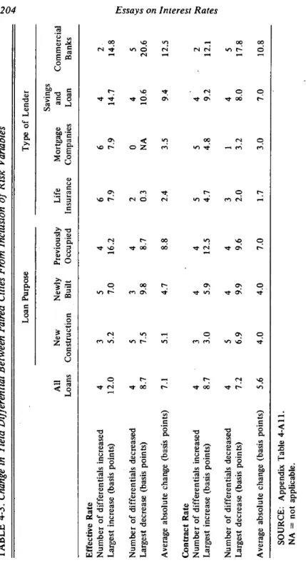
Table 4-3 indicates that both increases and decreases in yield
differ-entials between paired cities can be expected to arise with the
intrO-duction of risk variables, but that for all loans combined the changes
will ordinarily be small. The differential widened in four cases and
narrowed in four cases in the effective rate comparisons, with changes
ranging up to 12 basis points but averaging only 7 basis points. Among
categories of loan purpose, the largest increase, 16 basis points, arose
in the previously occupied group.
The influence of risk
variables on yield
differentials
isclearly
dependent upon the lender category.
Differentials between interest
rates in paired cities generally increased slightly, when differences in
contract terms were taken into account, for loans by life insurance
companies and mortgage companies. For loans by savings and loan
associations, the changes were greater, averaging over 9 basis points,
representing four increases and four declines. On commercial bank
loans five of the differentials decreased and only two increased. Changes.
averaged 12.5 basis points, with three decreases ranging to over 20
basis points.
For all lender groups and categories of loan purpose the changes
that result when risk variables are considered are slightly lower in the
contract rate data than in the effective rate data.
Yield differentials between paired cities as measured from regression
coefficients were also compared with the raw data, in which neither
loan purpose nor lender type is held constant. The yield differential
was larger in the unadjusted data for six of the eight sets of paired
cities; the average of the eight differences was nearly 10 basis points,
and the largest was 16 basis points.
INTRAREGIONAL MORTGAGE YIELD DIFFERENTIALS
Chart 4-1 presents frequency distributions of average effective interest.
rates in 100 SMSAs, divided into four regions. Data appear in Table
4-4. These distributions show that yield differentials of 50 basis points
or more between cities in the same region are not uncommon.
TABLE 4-3. Change in Yield Differential Between Paired Cities From Inclusion of Risk Variables
: AU Loans Loa n Purpose Type of Lender New Construction Newly Built Previously Occupied Life Insurance Mortgage Companies Savings and Loan Commercial BanksEffective Rate Number of differentials increased Largest increase (basis points)
4 12.0 3 5.2 5 7.0 4 16.2 6 7.9 6 7.9 4 14.7 2 14.8
Number of differentials decreased Largest decrease (basis points)
4 8.7 5 7.5 3 9.8 4 8.7 2 0.3 0 NA 4 10.6 5 20.6
Average absolute change (basis points)
7.1 5.1 4.7 8.8 2.4 3.5 9.4 12.5
Contract Rate Number of differentials increased Largest increase (basis points)
4 3 8.7 3.0 . 4 4
59
12.5 5 4.7 5 4.8 4 9.2 2 12.1Number of differentials decreased Largest decrease (basis points)
4 7.2 5 6.9 4 9.9 4 9.6 3 2.0 1 3.2 4 8.0 5 17.8
Average absolute change (basis points)
5.6 4.0 4.0 7.0 1.7 3.0 7.0 10.8
SOURCE: Appendix Table 4-All. NA =
not
CHART 4—i. Distribution of Effective Interest Rate for All Loans by
Geographic Area, 100 Metropolitan Areas
Obser-B Mean I -... .1
1N27
-2 — :::::::::: 0— — — —
{ .1 1 Mean i i i i i — 8 6 -Midwest4
-1—
a 1407 -2 — ::::::::::::::l:.:::.:.:::::::::. ::::::;::: — 0 , , Mean Mean -0• M. —r:.:1
N;
:
+a-86-
4-
2-0_.
5.3 I I I I 5.5 West N 21 = 6.2780 a-= .2794 5.7 5.9 6.1 6.3 6.5 6.7 6.9 Interest rate206
Essays on Interest Rates
TABLE 4-4.
Distribution
of Mean Effective.Inrerest Rates on All Loans in
100 Metropolitan Areas, by Geographic Areas, May—December 1963
(number of observations)
Rate Class East Midwest South West All Areas
5.30—5.39 1 — — — 1 5.40—5.49 3 — — — 3 5.50—5.59 5 — — — 5 5.60—5.69 + 5 — — — 6 5.70—5.79 7 6 1 — 13 5.80—5.89 4 6 3 1 14 5.90—5.99 1 - + 6 3 2 ÷ 12 6.00—6.09 1 8 4 — 13 6.10—6.19 — 5 6 6 17 6.20—6.29 — — 2 ÷ 6 8 6.30—6.39 — — — — — — 6.40—6.49 — 2 2 4 6.50—6.59 — — — 1 1 6.60—6.69 — — — 1 1 6.70—6.79 — — — 1 1 6.80—6.89 — — — 1 1 Mean rate 5.678 5.955 6.076 6.278 5.974 Standard deviation .236 .141 .196 .279 .300 Number of observations 27 31 21 21 100
NOTE: +indicatesmedian class.
West, a substantial degree of overJapping exists in the yield patterns
of the several regions. Rates of 5.8 to 6.1 per cent exist in cities
in all four regions. Finally, the regional differentials between the lowest
rate metropolitan area in the East and the highest in the West reach
one and one-half percentage points.
We further disaggregate data for 42 SMSAs grouped into five
re-Average rates and other terms for these areas are presented in
two sets of Appendix tables, the "VT" series and the "S" series, which
provide different levels of aggregation. The "T" series provides mean
data for all loans combined, for all five lender groups, and for the three
'3The New England states were broken out of the Eastern grouping to create
categories of loan purpose. The "S" series further disaggregates the
data, so that terms on loans in each loan purpose group by members
of each lender group can be compared. Both series provide mean
values of the seven available contract terms for any cell in which at
least six observations were recorded. Cells in which 6—lO observations
were available are starred.'4
These tabulations demonstrate that a map of mortgage yields
pre-sents a checkered, rather than an orderly, regional pattern even within
a given category of lender type and loan purpose. This point is
illus-trated below by selected comparisons from Appendix Table 4-Si of
some intraregional and interregional yield differentials covering loans
on newly built homes by savings and loan associations.
Geographical Yield Differentials
ml
raregional
Basis Points
Interregional
Basis Points
Boston-Hartford
43
Boston-New York
42
Providence-New Haven 38
Chicago-New York
4
Detroit-Indianapolis
22
Chicago-New Orleans
15Cincinnati-Cleveland
12Kansas City-Atlanta
27
Houston-Ft. Worth
21St. Louis-Seattle
21
Louisville—Atlanta
30
Cleveland-Houston
30
Seattle-Portland
17Boston-San Francisco
76
Denver-San Diego
31Atlanta-Los Angeles
5Intraregional yield differentials also can be measured by the
re-gressions covering 18 major metropolitan areas. Effective yield
differ-entials (in basis points) between four pairs of cities, one pair in each
of the major regions, are shown below for both all loans and loans
on newly built homes by savings and loan associations:
The
terms presented are mean effective interest rate
Tables 4-TI,
4-Si), mean contract rate (4.T2, 4-S2), average fees and charges (4-T3, 4-S3),
average loan-value ratio (4-T4, 4-S4), mean purchase price (4-T5, 4-S5), mean
loan amount (4-T6, 4-S6), and average maturity (4-T7, 4-S7). Ordering of
cities within each region in the T and S series is based upon mean effective
interest rate secured by savings and loan associations for mortgages on previously
208
Essays on interest Rates
Savings and Loan
All Loans,
on Newly Built
Differential
Homes, Differential
Based on
Based on,
Regressions
Regressions
Average
With Risk
Average
With Risk
Region
Cities
Rate
Variables
Rate
Variables
East
New York
less
Philadelphia
1232
17
29
Midwest
Cleveland
less
Detroit
4
11 324
South
Dallas
less
New Orleans
27
2123
22
West
Los Angeles
less
Seattle
27
24
1328
It is clear that the risk variables included in the regression do not
explain these intraregional differentials. In both sets of pairings the
yield differentials are larger after inclusion of risk variables for three
of the four sets of paired cities. Differences in mortgage yield
deter-minants not included in our data, including factors, bearing on local
market structure, may be responsible for this.
FACTORS UNDERLYING YIELD DIFFERENTIALS
The existence and approximate magnitude of mortgage yield
differen-tials both between and within regions have been established; we now
consider possible factors underlying these differences.
The mortgage market is essentially a local market, matching local
savings with local housing demands. Assuming no capital flows between
markets, uniform mortgage yields would arise only if demand and
supply curves for mortgage capital intersected at the identical interest
rate in all areas. This would require essentially uniform local demand
and supply curves throughout the United States, which implies, among
other things, uniform rates of population and economic growth; such
conditions are not met in the American economy.
Guttentag has reduced the situation to its essentials: "The most
important determinant of the demand for mortgage funds is growth
in the number of households, while the supply of funds is largely
deter-mined by the size of the sitting population. For this reason, the demand
in areas experiencing a large net immigration of population will be
greater, relative to supply, and interest rates will be higher than in
'old' areas where population is growing slowly or not at all. This is
the principal cause of regional yield differentials."5
The major question is why the market does not entirely eliminate
the differentials through intermarket flow.
High Cost of In formation
Information on average loan characteristics for various areas is not
difficult to obtain. Average terms on new commitments in major cities
are published monthly by both House and Home and the Federal Home
Loan Bank Board. Additionally, mortgage investors are a gregarious
group, frequently meeting with colleagues in the city, county, state,
region, and nation. Consequently, most competent mortgage lenders
have a fairly accurate picture of interest rate patterns in the areas in
which they operate. For life insurance companies and some large
savings banks, this area encompasses most of the United States.
Information on specific loans, however, is costly to obtain. Although
some economists may be surprised by the fact, most national lenders
in the mortgage market insist upon personally visiting every residential
property upon which they make conventional loans. They are reluctant
to surrender authority for firm commitments to agents.1° To many
lenders a personal assessment of the borrower's willingness to fulfill
his obligation is the most important factor in a mortgage commitment.
The cost of personal interviews increases with both distance and the
number of areas selected for foreign investment. Thus, information
regarding the quality of a loan in a distant area is likely to cost more
than comparable information on local conditions.
Jack
M. Guttentag, "The Federal National Mortgage Association," in Federal
Credit Agencies, Englewood Cliffs, 1963, p. 135.
An investor who has corresponded for some years with a mortgage banker
may purchase the loan without inspecting the property, but he will visit it within
six months, with an option to return the loan to the originator.
210
Essays on Interest Rqtes
Legal Constraints
Legal factors that affect lenders' ability and willingness to make
out-of-state conventional mortgage loans may be classified into two
cate-gories—those that serve as a barrier to capital flowing from the state,
and those that inhibit or influence the flow of foreign mortgage funds
into the state.
The first category of statutes governs out-of-state lending by domestic
institutions. In general, these statutes allow life insurance companies
nationwide lending powers, but restrict
lending by other
types of financial institutions. Savings and loan associations have
gen-erally been limited to an area bounded by a
50
or 100 mile radius
from the home office.
The 19 states that have chartered mutual savings banks fall into
three groups. Connecticut, Massachusetts, and New Jersey allow
out-of-state lending within only a limited radius. Currently, the range in
New Jersey is 50 miles from the state border and, in Connecticut and
Massachusetts, 50 miles from the home office.17 Five states limit
out-of-state lending by mutual savings banks to a group of states, usually
contiguous
states. The remaining states permit virtually
unlimited
out-of-state lending powers, although maximum contract terms may
be specified. Although the principal savings bank state, New York,
presently falls within this category, in 1963 lending activities were
restricted to New York and adjoining states.
The second category of statutes, which may influence the transfer
of funds to a foreign state, is more complex. A lender must consider
the doing business statutes, registration and qualification requirements,
and franchise and income taxes. Some states make it relatively easy for
a foreign corporation to engage in mortgage lending, others require
some comparatively simple and inexpensive procedures, some require
onerous and/or expensive procedures, and a number of states prohibit
entirely loans by certain types of foreign lenders. For example,
Ala-bama, Arizona, Colorado, and New Hampshire do not permit
out-of-state savings and loan associations to make mortgage loans.18
The permissible area for both Connecticut and New Jersey savings banks
has been broadened since 1963.
See
Malcolm C. Sherman, Mortgage and Real Estate Investment Guide,
which is published annually by Helen B. Sherman, Boston, Massachusetts. Much
of the material in this section is drawn from the 1967 edition of the Guide.
Sherman includes (on pp. 407—408 of the 1967 edition) a summary of the ease
Legal limits on loan characteristics may affect foreign lending in a
state. Both maximum allowable interest charges and penalties for
usurious rates differ widely among states. In early 1967, maximum
interest rates ranged from 6 per cent (10 states) to 21 per cent (1
state).1° Some states impose civil penalties only, but these range from
loss of excess interest, to loss of all interest, to loss of principal and
inter-est. The effect of fees and charges on the determination of usury varies in
similar fashion. Finally, in some states interest on interest is prohibited,
which causes complications for the lender in the assessment of penalties
for delinquent payments. Statutory limits on loan size, loan-value ratio,
and maturity also vary from state to state.
The foreign lender must be familiar with the detail of the real
property laws, because of the importance of assuring adequate security.
"The rights of husband and wife, courtesy, dower and homestead are
pertinent in making mortgage loans in the various states, especially
where one of the parties does not execute the mortgage and the other
claims sole ownership of the security."20
Of major importance are the remedies available to the mortgagee
in the event of default and/or foreclosure. For example, in Louisiana,
if a monthly payment is not paid within 31 days of the due date, the
property may be immediately foreclosed and sold; there is no equity
of redemption. In other states,
it may be several years before the
of making out-of-state mortgages by foreign corporations. He rates each state,
on an A (easiest) to E (prohibited) scale, on the basis of the aggregate effect
of state statutes, in his opinion, on mortgage loan activities of seven types of
lending institutions. See also John J.
Redfield, "Out-of-State Mortgage
Invest-ments by Savings Banks," Commercial and Financial
Chronicle, January 5, 1956.
The complete distribution follows: 6 per cent—lO states; 7 per cent—6 states;
8 per cent—12 states and D.C.; 9 per cent—I state; 10 per cent—li states; 12
per cent—6 states; 21 per cent—i state; no limit—Maine, New Hampshire,
Massachusetts.
(Source: memorandum from
the legal department, NationalAssociation of Mutual Savings Banks, March 29, 1967.) Since credit was
rela-tively easy during the period under study, usury statutes were of limited
signifi-cance. Tn 1967, however, foreign residential mortgage capital virtually ceased
flowing into a number of Southern states with 6 per cent ceilings. North Carolina,
under pressure from mortgage bankers and home builders, raised the rate limit
to 7 per cent in June of 1967.
During the extremely tight credit conditions that obtained during 1967, usury
statutes probably contributed to interstate capital flows. New York savings banks,
faced with a 6 per cent limit on conventionals when FHA-insured loans were
selling at 6 per cent plus five, to eight' points, took advantage of legislation
allow-ing nationwide conventional lendallow-ing' and poured mortgage money into states
allowing higher yields. The situation was comparable in Pennsylvania.
212
Essays on Interest Rates
redemption period has expired and a clear title can be passed to a
subsequent purchaser. Discussions with a large number of mortgage
bankers indicate that the diversity of foreclosure and equity of
redemp-tion statutes is the single most important barrier, if one is to be singled
out, to a larger interstate flow of mortgage capital, and certainly to
the development of a secondary mortgage market.
Varying Costs of Acquisition and Servicing
Facilities for the acquisition and servicing of residential mortgages are
not uniformly available. A sparsely settled area may simply not justify
the cost of establishing a mortgage company or branch office of a bank
or life company. The consequence is pockets of capital scarcity that
can be found in rural areas and small cities throughout the United
States. They are often characterized by a local financial monopoly,
perhaps a single savings and loan association, or a commercial bank
and savings and loan with close ties. This lack of technical facilities for
capital transfers is the principal source of intraregional differentials.
Facilities do exist for interregional fund transfers to capital-deficit
areas, but in mortgage lending they often involve higher processing
costs than local lending. This is largely a result of duplication of
facili-ties and services when a mortgage banker is retained; the amount
depends upon the degree to which the lender is
willing to delegate
lending authority. Auditing procedures for assuring the financial
sound-ness of the servicing agent also increase the total cost of foreign lending.
SUMMARY AND CONCLUSIONS
This paper has considered the influence of property location on effective
yields of
conventional, residential mortgage yields during
1 963.Property location is shown to be a statistically significant yield
deter-minant. This is true of loans by five types of lender and for three
categories of loan purpose. Property location
isleast significant for
loans on newly built homes, which represent a more homogenous class
than the new construction and previously occupied categories.
Interregional mortgage yield differentials are largest in magnitude
when measured between average interest rates prevailing in the East
and West. The differential of approximately 70 basis points in effective
which existed
in
1940. On the most standardized property type, newly
built homes, the differential between Eastern and Western average rates
is slightly less than one-half of one percentage point.
A large part of the East-West differential
in mortgage yields
isattributable to differences in mean rates on loans by savings and loan
associations. For this lender group, effective interest rate in the West
averages 65 basis points higher than in the East. In contrast, the average
differential for three other lender groups—life insurance companies,
mutual savings banks, and commercial banks—is only one-quarter
of a percentage point.
This would appear to enlarge, rather than diminish, the economic
significance of the interregional differential because savings and loan
associations represent the principal source of conventional residential
mortgage financing. For many borrowers they may be the only practical
source. The most important consideration to most borrowers seeking
home financing is the down payment required, and savings associations
typically are authorized to allow a higher loan-value ratio than
com-peting lenders. There is some evidence that borrowers who require
a loan in excess of 75 per cent of property value pay a market premium
for the privilege, particularly in areas where capital demand exceeds
supply. Whether lender risk exposure rises correspondingly is
question-able.
The continued existence of interregional yield differentials appears
to represent a manifestation of allocational inefficiency within an
im-portant segment of the
financial markets.21
Whether
it
isserious
enough to warrant official concern is a matter of personal
determina-tion. There are indications, however, that some mortgage interest rate
variation could be reduced if existing obstacles in the path of interstate
mortgage capital transfers were removed. Specifically, state laws should
be redrawn to increase the mobility of mortgage capital. A uniform
real property code would reduce the reluctance of lenders to engage
in widespread out-of-state mortgage lending activities. A corresponding
requirement is that geographical lending authority of the various
finan-cial institutions be broadened to permit nationwide mortgage lending.
21Without knowledge of transaction costs, of which information costs relatingto
the lender's risk are often the most important, we cannot make
acon-clusive determination of allocative inefficiency. George J. Stigler's remarks in "Imperfections in the Capital Market," Journal of Political Economy, June 1967, pp. 287—292, are most relevant here. But the local-monopoly-structure of a good
deal
of the
residential mortgage market does suggest the opportunity for214
Essays on Interest Rates
Intraregional yield differentials of substantial magnitude were also
established. These arise not only across state lines but also between
neighboring cities within individual states. Additionally, within
indi-vidual metropolitan areas, significant differences in rates charged by
different 'types of lenders are evident. In conclusion, it would seem
that structural changes are required in a relatively large number of
local residential mortgage markets.
APPENDIX TABLE 4-Al. States Included in Regions
REGION ONE -East REGIONTHREE (cont'd)
Connecticut Georgia
Maine Kentucky
Massachusetts Louisiana
New Hampshire ' Maryland
New Jersey Mississippi
New York North Carolina
Pennsylvania Oklahoma
Rhode Island South Carolina
Vermont Tennessee
Texas
REGION TWO — Midwest Virginia
Illinois Washington D. C.
Indiana West Virginia
Iowa Kansas
Michigan REGION FOUR —West
Minnesota Alaska
Missouri Arizona
Nebraska California
North Dakota Colorado
Ohio Hawaii
South Dakota Idaho
Wisconsin Montana
Nevada
REGION ThREE —South New Mexico
Alabama ' Oregon
Arkansas Washington
Delaware Wyoming
APPENDIX TABLE 4-A2. Mean Effective Interest Rate for Type (standard deviations in parentheses)
States, Grouped by Region, Loan Purpose, and Lender
All Loan Purpose Type of Lender New Newly Previously Life Mortgage Savings Mutual Commercial Loans Construction Built Occupied Insurance Companies and Loan Savings Banks Northeast Connecticut 5.67 5.69 5.67 5.67 5.52 — 5.84 5.62 5.62 (.25) (.24) (.25) (.25) (.10) (.27) (.22) Maine 5.86 (.29) 5.84 (.23) — 5.87 (.30) — — 5.89 (.20) 5.84 (.24) Massachusetts 5.43 (.27) 5.46 (.27) 5.37 (.27) 5.44 (.27) 5.22 (.08) — 5.58 (.28) 5.40 (.25) New Hampshire 5.89 (.22) 5.86 (.29) 5.89 (.19) 5.89 (.20) -_ — 5.93 (.19) 5.89 (.22) 5.84 Rhode Island 5.63 (.27) 5.65 (.27) 5.62 (.25) 5.63 (.27) — — 5.76 (.32) 5.52 (.14) Vermont 5.86 (.25) — 5.89 (.24) — — 5.88 (.22), —
Middle Atlantic Delaware 5.52 (.35) 5.53 (.40) 5.50 (.30) 5.54 (.36) 5.32 (.15) — 6.22 (.22) 5.38 (.24) 5.64 Maryland 5.70 (.33) 6.00 (.28) 5.61 (.28) 5.66 (.33) 5.44 (.15) 5.54 (.16) 5.83 (.31) 5.39 (.16) 5.68 (.32) New Jersey 5.73 5.76 5.68 5.75 5.52 5.72 5.80 5.74 5.63 • (.29) (.29) (.28) (.29) (.08) (.33) (.27) (.31) New York 5.79 (.28) 5.86 (.28) 5.82 (.27) 5.76 (.27) 5.55 (.11) 5.98 (.24) 5.90 (.24) 5.75 (.25) 5.69 (.28) (continued)
APPENDIX TABLE 4-A2 (continued)
All Loan Purpose Type of Lender New Newly Previously Life Mortgage Savings Mutual Commercial Loans Construction Built Occupied Insurance Companies and Loan Savings Banks Pennsylvania 5.73 5.86 5.58 5.76 5.44 5.54 5.89 5.40 5.76 (.35) (.33) (.32) (.35) (.22) (.29) (.32) (.18) (.32)Great Lakes Illinois 5.91 (.42) 5.95 (.45) 5.81 (.39) 5.92 (.41) 5.49 (.24) 5.42 (.17) 6.01 (.38) 5.57 (.35) Indiana 6.01 (.34) 6.02 (.36) 5.90 (.31) 6.03 (.33) 5.48 (.22) 5.58 (.14) 6.11 (.27) — 5.79 (.35) Michigan 5.85 (.34) 5.79 (.33) 5.75 (.29) 5.90 (.36) 5.50 (.16) 5.79 (.29) 5.86 (.29) — 5.94 (.46) Ohio 5.96 (.40) 6.03 (.39) 5.82 (.35) 5.98 (.41) 5.52 (.18) 5.51 (.15) 6.12 (.35) — 5.67 (.32) Wisconsin 5.85 (.32) 5.81 (.34) 5.88 (.29) 5.86 (.31) 5.38 (.17) 5.45 (.21) 5.93 (.28) 6.04 (.14) 5.70 (.32)
Upper South Kentucky 6.00 (.26) 6.02 (.25) 5.93 (.25) 6.04 (.25) 5.62 (.15) — 6.04 (.23) — 5.83 (.31) Tennessee 6.03 (.31) 5.94 (.34) 6.02 (.31) 6.08 (.29) 5.50 (.22) 5.71 (.19) 6.13 (.24) — 6.05 (.30) Virginia 5.90 (.30) 6.00 (.28) 5.84 (.31) 5.88 (.29) 5.53 (.22) 5.50 (.11) 5.98 (.26) 5.25 (.00) 5.83 (.28) West Virginia 6.05 (.23) 6.02 (.24) 5.99 (.21) 6.10 (.23) 5.72 (.18) — 6.11 (.18) — 5.93 (.28)
I
(continued)APPENDIX TABLE 4-A2 (continued)
All Loan Purpose Type of Lender New Newly Previously Life Mortgage Savings Mutual Commercial Loans Construction Built Occupied Insurance Companies and Loan Savings BanksLower South Alabama 6.35 (.58) 6.42 (.59) 6.19 (.48) 6.55 (.67) 5.43 (.21) 5.72 (.16) 6.59 (.35) — 7.22 (.79)
Arkansas Florida Georgia Louisiana
6.60 (.51) 6.17 (.33) 6.29 (.47) 6.22 (.60) 6.70 (.56) 6.20 (.35) 6.29 (.45) 6.22 (.62) 6.38 (.46) 6.14 (.29) 6.15 (.40) 5.94 (.43) 6.75 (.46) 6.17 (.34) 6.44 (.50) 6.31 (.62) 5.64 (.16) 5.74 (.31) 5.55 (.29) 5.42 (.25) — 5.95 (.23) 5.67 (.11) 5.56 (.19) 6.69 (.41) 6.21 (.31) 6.37 (.40) 6.34 (.56) — — — — — 6.39 (.48) 6.47 (.68) 5.92 (.57) Mississippi 6.41 (.62) 6.21 (.60) 6.23 (.59) 6.68 (.56) 5.45 (.31) — 6.58 (.49) — — North Carolina 6.05 (.22) 6.03 (.24) 6.04 (.25) 6.08 (.17) 5.47 (.26) — 6.09 (.15) 5.73 (.23) South Carolina 6.20 (.41) 6.21 (.37) 6.02 (.31)-6.28 (.46) — — 6.21 (.40) — — Plains Iowa 6.05 (.34) 5.98 (.37) 6.11 (.43) 6.06 (.29) 5.55 (.13) 5.69 (.29) 6.15 (.28) — 5.87 (.30) Kansas 6.09 (.35) 6.05 (.35) 5.99 (.34) 6.14 (.34) 5.53 (.21) 5.65 (.17) 6.13 (.31) — 5.96 (.50) (continued)
APPENDIX TABLE 4-A2 (continued)
All Loan Purpose Type of Lender New Newly Previously Life Mortgage Savings Mutual Commercial Loans Construction Built Occupied Insurance Companies and Loan Savings Banks Minnesota 5.83 (.33) 5.90 (.33) 5.70 (.28) 5.83 (.33) 5.49 (.16) 5.58 (.24) 5.95 (.25) 5.56 (.13) 5.68 (.39) Missouri 6.12 (.49) 6.24 (.53) 5.93 (.37) 6.18 (.50) 5.44 (.17) 5.77 (.21) 6.20 (.41) — 6.08 (.63) Nebraska 6.00 (.33) 5.93 (.23) 5.92 (.36) 6.07 (.37) 5.58 (.15) — 6.04 (.29) — 6.08 (.57) North Dakota 6.19 (.31) 6.41 (.34) 6.04 (.14) 6.15 (.29) — — 6.20 (.30) — 6.24 (.41) South Dakota 6.12 (.30) 6.06 (.34) 6.05 (.26) 6.18 (.28) — 5.71 (.17) 6.16 (.24) — —South West Arizona 6.31 (.45) 6.29 (.64) 6.24 (.34) 6.35 (.44) 5.48 (.24) — 6.43 (.34) — — New Mexico 6.12 (.42) 5.94 (.32) 6.10 (.32) 6.39 (.64) 5.48 (.24) — 6.25 (.32) — — Oklahoma Texas 6.07 (.51) 6.29 (.56) 6.08 (.51) 6.19 (.48) 5.87 (.39) 6.17 (.43) 6.28 (.54) 6.45 (.67) 5.45 (.23) 5.54 (.22) — 5.77 (.21) 6.21 (.43) 6.35 (.52) — 5.82 (.63) 6.42 (.78)
Rocky Mountains Colorado 6.25 (.52) 6.33 (.55) 6.13 (.43) 6.29 (.54) 5.60 (.15) 5.76 (.18) 6.41 (.47) — 5.91 (.45) 00 (continued)
APPENDIX TABLE 4-A2 (concluded)
All Loan Purpose Ty pe of Lender New Newly Previously Life Mortgage Savings Mutual Commercial Loans Construction Built Occupied Insurance Companies and Loan Savings Banks Idaho 6.08 (.23) 6.09 (.13) — — 6.05 (.16) — — — . — Montana 6.11 (.49) 6.20 (.43) 5.84 (.21) 6.21 (.64) 6.05 (.13) — 6.20 (.53) — 5.67 (.12) Utah Wyoming 6.23 (.39) 6.42 6.35 (.29) — 6.19 (.37) — 6.20 (.43) 6.49 5.76 (.36) — — — 6.35 (.26) 6.13 — — 6.14 (.53) 6.78 • (.61) • (.58) (.33) (.53)Far West California 6.41 (.49) 6.70 (.58) 6.16 (.43) 6.41 (.45) 5.58 (.25) 5.70 (.34) 6.51 (.42) — 5.99 (.34) Nevada 6.20 (.39) — 6.07 (.03) -. — — — — 6.14 (.23) Oregon 6.19 (.47) 6.23 (.49) 5.97 (.30) 6.23 (.49) 5.65 (.23) 5.60 (.12) 6.30 (.44) — 5.92 (.30) Washington • 6.20 (.44) 6.30 (.37) 5.96 (.34) 6.22 (.50) 5.70 (.33) 5.89 (.33) 6.37 (.39) 5.87 (.22) 6.10 (.50)
NOTE: Cells with less than 15 observations are excluded. This nine-region breakdown is that recommended by the Conference on
APPENDIX TABLE 4-A3. Average Terms on Conventional Residential Mortgage Loan by Loan Purpose and Type of Lender for 18 Principal Metropolitan Areas Combined, May-December, 1963 (standard deviations in parentheses)
Contract Effective Loan Loan/Value Purchase Interest Fees and Interest Maturity Amount Ratio Price Rate Charges Rate (years) (dollars) (per cent) (dollars) (per cent) (per cent) (per cent) All observations 22.57( 4.96)
16,508 (7,815.6) 72.19