TWO ESSAYS IN ASSET PRICING
BY
JANGWOOK LEE
DISSERTATION
Submitted in partial fulfillment of the requirements for the degree of Doctor of Philosophy in Finance
in the Graduate College of the
University of Illinois at Urbana-Champaign, 2017
Urbana, Illinois Doctoral Committee:
Professor Timothy C. Johnson, Chair, Director of Research Professor Heitor Almeida
Associate Professor Alexei Tchistyi Assistant Professor Dana Kiku
Abstract
The first essay, Knowledge Capital and Innovation Efficiency Effects on Stock Returns, pro-vides a novel framework for understanding innovation in the asset pricing literature. Prior research shows that stock returns are increasing in firms’ innovative efficiency. In a dynamic model of investment in physical and knowledge capital, this effect can arise rationally as innovative efficiency amplifies risks associated with investment and investors require com-pensation for these risks. I identify operating leverage and expansion option channels as the main drivers of the risk premium. Simulations of panels of firms with heterogeneous technology can reproduce the economic magnitude of the empirical return effect. The model further implies that the effect should be stronger for firms with high operating leverage and low book-to-market ratios. These predictions are supported by the data.
The second essay,Operating Leverage, R&D Intensity, and Stock Returns, studies interac-tion effects of operating leverage and R&D intensity on stock returns. A producinterac-tion-based asset pricing model with knowledge capital has an implication that R&D intensive firms earn higher expected stock returns among high fixed costs firms. An investment strategy that bought R&D intensive firms and sold R&D weak firms earn 0.67% to 1.26% per month in high fixed cost portfolios, while the strategy is not profitable in low fixed costs portfolios. In regression analysis, one standard deviation increase in R&D expenditures is associated with 1.85% to 2.12% increase in yearly stock returns for above median fixed costs firms. By the recursive nature of knowledge capital accumulation, the value of knowledge capital itself is sensitive to the economic situation. R&D intensive firms’ values aggravate faster with fixed costs in bad times and investors require compensation for the risk. In short, the value of knowledge capital itself is risky, R&D intensive firms are more exposed to the risky nature of knowledge capital, and fixed costs amplify the risk.
Table of Contents
Chapter 1 Knowledge Capital and Innovation Efficiency Effects on Stock Returns . 1
1.1 Introduction . . . 1
1.2 Analysis of knowledge capital . . . 6
1.3 Model . . . 8
1.4 Model solution . . . 13
1.5 Simulation and results . . . 15
1.6 Isolating mechanism . . . 19
1.7 Testable Implications . . . 23
1.8 Conclusion . . . 25
1.9 Figures and Tables . . . 27
Chapter 2 Operating Leverage, R&D Intensity, and Stock Returns . . . 45
2.1 Introduction . . . 45
2.2 Model . . . 48
2.3 Empirical results . . . 53
2.4 Conclusion . . . 59
2.5 Figures and tables . . . 61
References . . . 70
Appendix A . . . 75
A.1 Numerical methods for chapter 1 . . . 75
Appendix B . . . 76
Chapter 1
Knowledge Capital and Innovation Efficiency Effects on
Stock Returns
1.1
Introduction
In recent years, neo-classical investment-based models have been successful in explaining the relation between firm characteristics and expected stock returns through the firms optimal choice of the physical capital investment. Even though the physical capital is one of the most important components of firm operation, the standard investment-based models lack many other meaningful aspects of firms decision process.1 Research and Development (R&D) is one of the essential activity for firms to increase their productivity by improving product quality, reducing production costs, or expanding the market (Hall, Mairesse, and Mohen, 2009). And it involves optimal choices on how much firms should allocate their resources. R&D is of great significance in business both at the national level and at the firm level. USA spends 432 billion dollars on R&D in 2014, which is 2.74% of the GDP2 and firms that perform R&D spend 3.5% of their sales on R&D on average. Especially, computer and electronic products industry or pharmaceuticals and medicines industry spend up to 10.2% - 13.4% of sales in 2014.3
This paper investigates R&D expenditures, physical capital investment and the expected stock returns under the neo-classical framework. I propose a new framework to consider the R&D decisions and knowledge capital and deliver the recently reported empirical regularity about R&D and stock returns. By the sensitivity analysis of the model, I isolate the mech-anisms that incur the effect. I also draw the implications for stock returns from the model and present evidence in the data.
1There had been models employing other components of production. I will discuss later. 2http://www.oecd.org/sti/inno/researchanddevelopmentstatisticsrds.htm
R&D has been a subject of an empirical asset pricing literature since Chan, Lakonishok, and Sougiannis (2001) find that firms with high R&D expenditures earn higher stock returns. Li (2011) reports that the positive relationship between R&D and stock returns are stronger for firms with financial constraints. Gu (2015) shows that market competition has the interaction effect with R&D. Many studies focus on the relationship between quantities of R&D and stock returns. Instead, this paper pays attention to the quality of R&D; that is, how well firms operate R&D with the same dollar amount spent.
Hirshleifer, Hsu, and Li (2013) show that innovative efficiency, measured by patent cita-tions over R&D expenditures or by the number of patents over the cumulative sum of R&D, predicts higher stock returns. Table 1 shows primary results of the Hirshleifer, Hsu, and Li (2013). It reports the Fama-Macbeth (1973) return regression on innovative efficiency. As innovative efficiency (IE) rises by one standard deviation, stock returns increase by 0.08% to 0.11% per month after controlling for other firm characteristics.4 They document that mispricing plays a role in the positive relationship between innovation efficiency and stock returns. Investors do not fully understand the complex technologies of the firm. As a result, Innovation efficient firms draw limited attention, and the stock price is undervalued.
This paper constructs the model that can explain innovative efficiency effects on stock re-turns in the neoclassical framework. It needs not imply investor’s limited attention. Agents’ rational decisions on R&D and investments can drive such effect.
I extend an investment-based model by incorporating both endogenous physical capital and knowledge capital.5 In most investment-based models, capital (physical, labor, knowl-edge etc.) evolves and depreciate linearly. It increases exactly as much as invested and depreciates proportionally. However, in this paper, knowledge capital has an alternative law of accumulation from the standard accumulation. I find the micro-foundation for knowledge capital accumulation function from applied microeconomics and management field. A large
4Hirshleifer, Hsu, and Li (2013) also perform portfolio analysis. The 66% high IE minus 33% low IE
portfolio yields about 35-46 basis points of Carhart-4 factor alpha per month.
5There have been extensions of investment-based models by employing an additional component of the
firm operation. Belo, Lin, Bazdresch (2014) consider labor and physical capital in the production function to account for the relation between hiring rate and stock returns. Lin (2012) adopts physical capital and intangible capital to explain the positive relation between stock returns and R&D expenditures. The model in this paper is different from the previous models in that it considers the quality of R&D and knowledge capital do not accumulate in the standard linear form.
body of research on R&D points out that the standard physical capital accumulation formula is not suitable for the knowledge capital build-up. It is because a standard accumulation of knowledge capital implies the negative relation between past R&D and current R&D, which is not consistent with the data. They suggest an alternative form that gets around the problem.6 Following those critiques and suggestions, I adopt the knowledge capital law of motion as follows.
zt+1 = eνt+1ztζz(1 +ht)ζh (1.1)
The next period knowledge capital zt+1 is determined by the current knowledge capital
zt and R&D expenditures ht ≥ 0, where νt+1 is an i.i.d. random shock on individual firm technology and ζz denotes depreciation rate of knowledge capital. The key parameter in
this equation is innovation efficiency ζh. It is the knowledge capital elasticity of R&D
expenditures. High ζh firms can achieve more in knowledge capital in the next period with
the same R&D spending than low ζh firms. This formulation can embody variations across
firms in the quality of R&D in addition to the quantity of R&D.
The existing knowledge and current efforts on increasing knowledge are complementary in generating additional knowledge. The knowledge capital that has been already acquired helps in producing new knowledge capital. This feature differentiates the knowledge capital from the standard setup of physical capital accumulation.
The first contribution of this paper is to explore what difference the equation (2.1) makes on firms’ policy decision and risk exposure. To understand the impact of the knowledge capital accumulation, I construct two simplified firms that only differ in the capital accu-mulation. One follows the standard linear capital accumulation and the other follows the knowledge capital accumulation form in equation (2.1). By comparing them, I find the opti-mal R&D expenditures increases more sharply with aggregate productivity than the physical capital investment. It is because R&D has an additional marginal benefit of enhancing the future operating environment. R&D expenditures become pro-cyclical, which is a stylized fact in the data. This characteristic makes knowledge intensive firms more sensitive to the
economic states.
Incorporating the feature of the knowledge capital, the model can quantitatively deliver the innovation efficiency effects under the realistic model setup. Firms choose both physical capital and knowledge capital simultaneously and the model includes many aspects of oper-ating environment such as quasi-fixed costs, time-varying risk premium7, which are standard in investment-based asset pricing literature. The model shows that the risk loading β rises with innovation efficiency.
The paper runs simulations to investigate if the model can reproduce the economic mag-nitude of empirical analysis. I run Fama-Macbeth regressions of stock returns on innovation efficiency with the simulated data. The result shows economically strong enough relation-ship between them after controlling for firm characteristics such as size, book-to-market ratio, and profitability. It is also consistent with the existing empirical regularities, such as book-to-market effects, and size effects.
To isolate the mechanism behind the result, I simulate the model with alternative param-eters. The main implication is that innovation efficiency intensifies the existing risk sources associated with the investment. The iterature has explored the risk sources of physical cap-ital investment. Carlson, Fisher, and Giammarino (2004) suggest operating leverage (OL) effects as one of the risk determinants. Operating leverage effect is that fixed(or quasi-fixed) costs make a firm value more sensitive to the economic states since the firm still have to pay the costs even in bad times. Knowledge capital provides investment opportunities and makes the firm more prosperous in good times, but in bad times, it does not provide as many opportunities as in good times. Thus, innovation efficient firms become more vulnerable to the fixed costs.
Hackbarth and Johnson (2015) document an expansion option effect. Investment oppor-tunities are like having real call options, firms expands (or exercise the options) when the prospect of the marginal increase in firm value is maximized over the adjustment cost. It means that firms are more likely to make an investment when firms can generate more cash
7Pricing kernel is given exogenously in this paper. The aggregate productivity fully determines the
dynamics of the pricing kernel. Agents do not care long-run consumption growth or stochastic volatility. I do not attempt to match aggregate moments or explain the predictability of market returns in this paper.
flow with a dollar spent on the capital. Those firms should exchange riskless cash to risk asset, and their firm values become more sensitive to the economic states. Innovation ef-ficient firms have more invest opportunities from knowledge capital, and it intensifies the expansion option effect.
I examine empirical evidence by testing the model predictions. The model suggests that innovation efficiency amplifies the operating leverage effect and expansion option effects. If the effect only comes from the investors’ limited attention, one should not be able to find any variation in the IE effect depending on operating leverage or the book-to-market ratio. When portfolios are formed by double sorting on OL and IE, the IE effects are stronger in high OL firms. Likewise, double sorts on book-to-market ratio and IE shows strong IE effect in low book-to-market firms. These results corroborate the channels that the model suggests.
My paper is based on the prior investment-based asset pricing model. Cochrane (1991) uses investment returns to understand stock returns. Zhang (2005) introduces the impacts of inflexibility on stock returns. Gomes and Schumid (2010) show how simultaneous decisions on leverage and investment can affect the systematic risk of the firm. Belo, Lin, and Baz-dresch (2014) investigate the impact of labor market frictions on stock returns. Hackbarth and Johnson (2015) analyze the positive relationship between profitability and systematic risk by the expansion and contraction option effects of investment.
Research on R&D is also closely related to my work as well. Griliches (1979), Hall, Mairess, and Mohnen (2009) survey huge literature on R&D and knowledge capital in economics. Hall, Griliches, and Hausman (1986), Klette (1996) attempt to measure the effects of R&D with different specifications from the cobb-douglas production function.
The outline is as follows. Section 2 analyze the effect of the alternative capital accumu-lation function. Section 3 discusses the full model that includes realistic aspects of firm operation. Section 4 calibrates and analyzes the solution of the model. Section 5 simulates the model and tests the simulated data in the same way as empirical papers would do. Sec-tion 6 investigates the economic intuiSec-tion of the model soluSec-tion and simulaSec-tion. SecSec-tion 7 analyzes the testable implications from the model with data. The final section concludes.
1.2
Analysis of knowledge capital
This section investigates the impact of the distinctive knowledge capital accumulation on firms’ policy and risk. I construct two versions of simple models that only differ in capital accumulation function. The first model accumulates capital linearly while the second model accumulates the capital as in equation (1). They represent the physical capital firms and knowledge capital firms, respectively. The model setup for both firms is as simple as possible to contrast the effect of the accumulation function clearly. By comparing two firms, I can show the difference in policy decisions between the impact of the knowledge capital accumu-lation and the standard physical capital accumuaccumu-lation. The purpose of this analysis is simply to contrast two firms. The models lack many aspects of the realistic operating environment such as capital adjustment cost, the time-varying price of risk, external financing costs, etc. Thus, the results are qualitative.
Table 2.1 panel (A) summarizes the model setup. Aggregate productivity follows mean reverting AR (1) process. The stochastic discount factor is the simplified version of full model SDF. The SDF has the constant Sharp ratio which does not embed the time-varying risk premium. The only difference between two firms is capital accumulation function and the profit scaling constant parameterκ in the knowledge capital firm. To enable comparing two different kinds of firms, I simulate both firms and set κ to match the long-run mean market value of two firms. Thus, they have the same market value at the steady state, and this makes the policies comparable in that the difference is not originated from the firm value.
The aggregate economy calibration is set as similar as possible to the full model, which mainly follows the calibration in Li, Lividan, and Zhang (2009). Table 2.1 panel (B) shows the calibration of the simple models. As the full model solution, the problems are solved by value iteration. The aggregate productivity Xt are discretized by Rouwenhourst (1995)
1.2.1
Policy comparison
The differential accumulation of physical capital and knowledge capital results in the dif-ference in policy decisions. Those policies have implications for firms risk dynamics. This section investigates the policy difference between physical capital firms and knowledge cap-ital firms and shows how knowledge capcap-ital firms can be more sensitive to the economics situation.
The figure 1.1 shows the investment and R&D policies of the two firms. Panel (A) and (B) represents the investment policy of physical capital firm and R&D expenditures policy of knowledge capital firm, respectively. In a good state of an economy, both firms increase their spending on the resources. It is notable that knowledge capital firm increases its expenditures much faster than the physical capital firm. Especially, when firms are in a small area, the increasing rate difference is huge. Knowledge capital firm raises R&D expenditures explosively when the economic situation reaches a certain level.
One can see the difference more clearly in panel (C) and (D). They are two-dimensional figures that plot the spending on capital when the firms are small (both k and z are 0.38) and large (both k and z are 8.30), respectively. Knowledge-capital firm increase R&D ex-penditures faster than investment of physical capital firm in panel (C). In the form of knowl-edge accumulation in equation (1), there is an extra marginal benefit of R&D expenditures in addition to the immediate increase in operating profit. It enhances the future operat-ing environment. The knowledge capital that has been already acquired helps to generate new knowledge capital. Thus, R&D expenditure rises sharply with aggregate productivity. Knowledge capital has a feature that could be more sensitive to the economic state.
Panel (D) shows not much difference in R&D expenditures and investment of large firms. R&D expenditures and investment are similar in panel (D). It is because the marginal benefit of existing knowledge capital decreases in size. As in equation (1), the next period knowl-edge capital is increasing and concave in the existing knowlknowl-edge capital. Although existing knowledge capital helps in generating new knowledge, the marginal impact of knowledge capital diminishes.
expenditures increase sharply as economic situation gets better. It is a stylized fact in the literature that R&D expenditures are pro-cyclical. Figure 2.1 plots the weighted average of R%D expenditures growth rate in Compustat universe and real GDP growth rate. The figure updates the survey in Barlevy (2007). The figure shows that the R&D growth rate is positively covarying with the real GDP growth. R&D growth rate tends to drop in NBER recession years. The correlation coefficient between R&D growth rate and the real GDP growth rate is 0.38 while the correlation between weighted average of Compustat capital expenditures growth rate and the real GDP growth rate is 0.3.
1.2.2
Expected excess returns
In this section, I show how expected excess returns vary depending on innovation efficiency. Figure 1.3 panel (A) plots the expected excess returns of firms that differ in innovation efficiency ζh. It shows that expected excess returns rise with the innovation efficiency. As
innovation efficiency increases, the increments in marginal benefit of R&D depending on economic states also rises. Thus, they spend more on R&D expenditures. Figure 1.3 panel (B) depicts that R&D-to-knowledge capital ratio increases with innovation efficiency ζh.
Innovation efficient firms make riskier choices on R&D than inefficient firms. Consequently, the values of those firms become more sensitive to the economic states.
The model in this section is too simplified to explain innovation efficiency effect enough. However, this model can illustrate how innovation efficiency that is embedded in knowledge capital accumulation can affect the firms’ risk and expected excess returns. The effect in this section is one source of the innovation efficiency effect, which amplifies the mechanisms that are suggested in the later section.
1.3
Model
1.3.1
Model
log mt+1 = logη+γt(xt−xt+1)
γt=γ0+γ1(xt−x¯)
0< η <1 is time discount parameter. Parameterγ0 >0, and γ1 <0 are constants which characterize the maximum sharp ratio. It increases with γ0. If γ1 = 0, the economy has the constant sharp ratio. With γ1 < 0, the maximum sharp ratio varies over time counter-cyclically. xt is aggregate productivity process in the economy. the pricing kernel solely
depend on xt, which is exogenously given. It follows AR(1) process.
xt+1 = ¯x+ρx (xt−x¯t) +σxxt+1 ¯
xis long run mean of aggregate productivity. ρx is persistence of the aggregate
productiv-ity. σx is volatility of the aggregate productivity. xt+1 is the aggregate productivity shock, which follows standard normal distribution.
Operating profit πi,t is
πi,t = extzi,tαzk αk
i,t −f ki,t
ki,t is physical capital and zi,t is knowledge capital. f is proportional costs to the physical
capital(quasi-fixed costs), 0 < αk < 1, and 0 < αz < 1 are output elasticity of physical
capital and knowledge capital, respectively. They govern how much output can be produced with the given amount of physical capital and knowledge capital. Physical capitalki,t follows
ki,t+1 =ii,t+ (1−δ)ki,t (1.2)
δ is depreciation rate for physical capital. ii,t is investment on physical capital. Firms
cannot divest their physical capital in this model. Investment, ii,t, should be greater than
zero, ii,t >0. There exists a physical capital adjustment cost, ci,t. It is as follows
ci,t = a 2 ii,t ki,t 2 ki,t
The adjustment cost is convex on investment and decreasing in physical capital. a is constant. This is standard set-up for the adjustment cost in the literature.
This paper differs from existing investment-based models in that knowledge capital, zi,t
is chosen endogenously. The knowledge capital determines the profitability of the firm. Firms should spend their resources on R&D to manage their profitability for every period. Recently, Kung and Schmid (2015) suggests the model that endogenizes R&D and innovation to explain aggregate returns. They adopt innovation sector that only innovates while final good sector buys the technologies from the innovation good sector. Their set up is for explaining aggregate level innovation and market returns. This paper, on the other hand, intends to describe a firm-level decision regarding innovation. I focus on how firms allocate resources on R&D, how much they get out of it, and its implication on the cross-sections of expected returns. The law of motion of knowledge capital is defined by
zi,t+1 = eνi,t+1zi,tζz(1 +hi,t)ζh (1.3)
νi,t+1 ∼ N(0, σν)
νi,t+1 is an i.i.d. random shock on the outcome of R&D. hi,t > 0 denotes R&D
expen-ditures. Divestment on knowledge capital is not allowed in this model. 8 ζz is future
knowledge capital elasticity of current knowledge capital. ζz can capture industry
compet-itiveness or depreciation rate of knowledge capital. ζh is the knowledge capital elasticity of
R&D expenditures, which is innovation efficiency in this model. This knowledge capital ac-cumulation distinguishes the model from other multi-factor models with another component of production. The distinctive features of knowledge are detailed in the discussion section.
When firms cannot finance investment and R&D with internal capital, external financing costs are incurred. An equity issuance cost, λ(ei,t) is
λ(ei,t) = (λ0 +λ1|ei,t|)I{ei,t<0}
λ0 is fixed issuance cost,and λ1 is variable issuance cost. I{ei,t<0} is an indicator function 8In practice, disinvestment in knowledge capital is not impossible in some sense, for example, sales of
that gives value one whenei,t <0, and gives zero otherwise.
Equity issuance,ei,t is
ei,t =πi,t−ii,t−hi,t−ci,t
Distribution to shareholders,di,t is
di,t =ei,t−λ(ei,t)
For each period, a manger maximizes firm valuev(ki,t, zi,t, xt) by choosing investment (ii,t)
and R&D (hi,t).
v(ki,t, zi,t, xt) = max
{ii,t,hi,t}
{di,t+E[mt+1v(ki,t+1, zi,t+1, xt+1)]} (1.4)
1.3.2
Discussion
This section discusses the setup of the model further in detail. This model assumes the pro-duction to be the Cobb-Douglas function. The motivation is endogenizing the profitability which is the residual value in the output functions of neo-classical models. Having Cobb-Douglas production function with knowledge capital is a natural extension of the neo-classical models.
Extending neo-classical models is not the only reason the model is set up the way it is. I find the empirical evidence about the relationship between knowledge capital and physical capital. The model implies that knowledge and physical capital are somewhat complementary. The more knowledge capital the firm has, the more investment opportunities available for firms. It naturally comes from the assumption of Cobb-Douglass function. Figure 1.5 shows that physical capital investment is high for innovation efficient firms. However, one of conventional thought is that IE efficient firms invest less in physical capital and, instead, spend much more on developing knowledge capital because their business is more focused on knowledge. One might think that knowledge capital and physical capital are kinds of substitutable. Many start-up firms in silicon valley might play a role to generate such stereotypes.
If knowledge and physical capital are complementary, the coefficients of IE should be positive. Table 2.2 presents regressions of investment on IE. One standard deviation increase in log(1+IE) is associated with about 0.15 % increase in log(1+Capx/at) with t-statistics 3.72 to 3.97. This implies that innovative efficient firms do invest more than inefficient firms, which is consistent with the model predictions.
Equation (1.3) is the crucial assumption that differentiates the model from other investment-based models. The knowledge capital accumulation is inspired by Hall and Hayashi (1989) and Klette (1996). Klette (1996) points out that it might not be realistic to apply the con-ventional capital accumulation (equation (1.2)) to the knowledge capital. With the standard specification, existing capital do not play a role in generating additional capital. However, the empirical analysis points out that existing knowledge gives the firm more incentives to spend on R&D (Hall, Griliches, and Hausman, 1986). On the other hand, multiplicative form as in equation (1.3) is different from the linear accumulation.
I assume 0< ζz <1 and 0< ζh <1. Under these assumptions, the knowledge capital has
the following characteristics.
zz0 >0, zh0 >0, zzz0 <0, zhh0 <0, zhz0 >0
z0 is the next period knowledge capital and subscripts are partial derivatives. Current knowledge makes easier for firms to advance their knowledge capital (zz0 >0). R&D expen-ditures increase future knowledge capital (zh0 > 0). Current knowledge capital and R&D expenditure is concave on future knowledge capital (zzz0 <0, zhh0 <0). Not like physical cap-ital accumulation, knowledge capcap-ital accumulation shows that the former successful R&D gives firms more incentives to invest on R&D (zhz0 >0). These characteristics are consistent with the literature in management and applied microeconomics. Recently, macroeconomics and finance areas adopt these features of knowledge and share the similar spirit. Comin and Gertler (2006) and Croce et al. (2016) shows R&D behavior that differs in output elasticity of R&D at macro-level and at firm-level.
1.4
Model solution
1.4.1
Calibration
Output elasticity of physical capital, αk and the elasticity of knowledge capital, αz are 0.6
and 0.3 respectively. αk is similar to Li, Lividan, and Zhang (2009). Output elasticity
of “knowledge capital” (αz) is set to make output elasticity of “R&D” be 0.045 for the
innovative inefficient firm and be 0.15 for the efficient firm. Prior research has tried to measure output elasticity of R&D at firm level or industry level. The calibration in this paper utilizes the previous empirical analysis. The elasticities vary mostly from 0.02 to 0.2 (Hall, 2009). Output elasticity of “R&D” is just output elasticity of knowledge capital times knowledge capital elasticity of R&D (αz ×ζh). In the baseline calibration, αz is set to 0.3.
Thus, I setζh0.15 for innovation inefficient firms so that output elasticity of “R&D” becomes
0.045, and set ζh 0.45 for innovation efficient firms so that output elasticity of “R&D” is
0.15.
The long run mean of aggregate productivity x is set to -3.2 to have the book-to-market ratio from simulated data to match the ratio from the data. Many of parameters follow calibration in Li, Lividan, Zhang (2009), the persistence of aggregate productivity ρx is
0.983. The standard deviation of aggregate productivity σx is 0.0023. Quasi-fixed cost, f is
0.01. Constant price of risk parameter γ0 is 50 and Time-varying price of risk parameter γ1 is -1000. This stochastic discount factor yields countercyclical time-varying risk premium. The physical capital depreciation rate δ is 0.01. Physical capital adjustment cost, a is 15. Time discount parameter η is 0.994. Fixed component of external financing cost, λ0 is 0.08. Proportional financing cost, λ1 is 0.025. Unfortunately, to my knowledge, no prior research estimates the parameters for knowledge capital. I set future knowledge capital elasticity of existing knowledge capital, ζz is 0.993. It is because knowledge capital depreciates slower
than physical capital does. I set standard deviation of knowledge capital accumulationσν is
0.01, which is larger than the volatility of aggregate productivity. It is reasonable to assume that building knowledge capital entails more uncertainty than the uncertainty of the entire economic productivity.
1.4.2
Value and policy functions
Figure 1.4 depicts the value function v(k, z, x), defined in equation (1.4). The shape of value is consistent with the existing literature and adds the another dimension, knowledge capital. Firm value increases with physical capital, knowledge capital, and aggregate pro-ductivity. The value functions are monotonically increasing and concave in both k and z. Many investment-based models show that firm values are increasing and concave in k. The firm value in is also increasing and concave in knowledge capital, z. Knowledge capital exhibits decreasing return to scale as well as physical capital does. Marginal contribution of knowledge capital to the firm value decreases as a firm accumulates knowledge capital; meanwhile, it gets easier for firms to innovate as in equation (1.3).
Firm values for good time (dash-dot line) in figure 1.4 are the values when the aggregate productivity is above the one unconditional standard deviation away from the mean. Firm values in bad time (dotted line) have the aggregate productivity the one unconditional standard deviation below from the average. When all other things are equal, innovation efficient firms have higher values than the inefficient firms.
Figure 1.5 shows investment and R&D policies as a function of physical capital. In all panels, both investment and R&D increases in good times and decreases in bad times. For IE firms (panel (B) and (D)), the impact of the economic situation is significant. Innovation efficient firms spend on R&D much larger in a good state while they cut down drastically on R&D in a bad time. IE firms have more investment opportunities and more substantial marginal benefit R&D in economic boom, but knowledge capital does not provide investment opportunities enough in bad times. In panel (C), economic states do not have effects very much on R&D policies for innovation inefficient firms. They barely spend on R&D regardless of the aggregate productivity. It is because innovation inefficient firms are better to spend on physical capital or dividends if internal capital is available. It is similar to the fact that many firms do not spend on R&D at all.
1.4.3
Beta
βi,t =
−Cov[ri,t+1, mt+1]
V ar[mt+1]
Following Li, Lividan, Zhang (2009), I can computeβ by backing it out from the following one factor beta-pricing equation.
E[ri,t] =rft +βi,tλmt
wherertf ≡1/E[mt] is the risk free rate, and λmt ≡V ar[mt+1]/E[mt] is the price of risk.
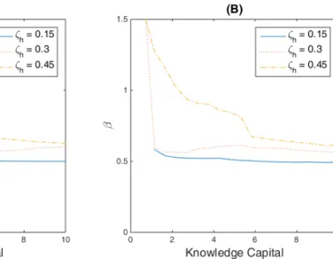
Figure 1.6 panel A shows β as a function of physical capital capital. I set the aggregate productivity at mean level and knowledge capital at the midpoint of the range. I depicted
βs when R&D efficiency,ζh are 0.15, 0.3, and 0.45. Solid line is the case ofζh = 0.15. dotted
line is theβ whenζh = 0.3. Dash-dot line is the case ofζh = 0.45. When all other things are
equal, β increases with innovation efficiency. This figure suggests that innovation efficient firms load more on risk, and consequently, they have higher stock returns
Figure 1.6 panel B shows β as a function of knowledge capital in case of ζh = 0.15, 0.3,
and 0.45. As in the panel (A), aggregate productivity is set to mean value and the physical capital is at the midpoint of the grid range. β increases with ζh in this direction as well.
The shape of β is a bit humped in the figure 1.6. In some state, the risk gets higher for large firms than the small firms. It might be related to the external financing costs. It is not reported in the paper but if firms do not incur external financing costs, humps in the beta figures disappear. Financing costs hinder firms’ investment and these bindings make the firms’ risk non-monotonic.
1.5
Simulation and results
I simulated 1000 panels for the benchmark model. Each panel has 5000 firms and 720 months. First 240 months are dropped to mitigate the effect of the initial conditions. I run well-known empirical analysis (Fama-Macbeth regressions) for each panel and calculate cross-panel averages of empirical results.
1.5.1
Unconditional moments
I report the unconditional moments of the model simulation in the Table 2.4. The overall fit seems acceptable. Moments that are related to the overall economy and risk premium, the annual average risk-free rate, and the volatility of annual risk-free rate are close to the data.
For the firm level moments, the annual investment-to-book-asset ratio is close to the data for both innovation efficient and inefficient firms. The efficient firm has higher annual R&D to book asset ratio than data, while innovation inefficient firm does not. However, when scaling down with the market value of asset, then the ratios for both firms are a little lower than the data. The book-to-market ratios higher than the average of data for inefficient firms and lower than the average for IE firms. Simulated data does not represent the entire firms. Instead, I compare the two groups (innovation efficient firms and inefficient firms). The moments need not have to be the same as the quantities or the entire market. The moments from the data lies in between the moments of two groups, and this supports that each group represents innovation efficiency well.
The average return on equity for both groups is higher than the data. It is because ROE from the model in the table 2.4 is actually defined as a profitability, (ki,t+1−ki,t+di,t)/ki,t. It
can be slightly different from the accounting measure, ROE. There might be many another type of costs for the net income in the accounting ROE so that it might lower the value. Another potential issue is that innovation inefficient firm has higher ROE than ROE of innovation efficient firm. It is because of decreasing-return-to-scale of physical capital. As R&D efficiency increases, more investment opportunities are open to the firm. The efficient firm grows faster and has more physical capital. The profitability measure is scaled by physical capital. Thus, it lowers the unconditional profitability of the IE firm. Size effect dominates the increase in knowledge capital effect.
The volatility of the investment and R&D to the market value ratio for both firms are lower than the data. It is because the simulated data does not represent entire economy. The simulated investment-book asset volatility is within-firm volatility. If there are many kinds of firms in the economy, then the unconditional moment will rise.
1.5.2
Innovation efficiency and expected stock returns
This section demonstrates with the model simulation that the IE effect rises rationally. I examine whether simulated data from the calibrated model can deliver the IE effect.
Table 2.5 presents the results of Fama-Macbeth regression (1973) with the simulated data from the baseline model. In column (1), the innovation efficiency effect is positive but not statistically significant. The investment-based model has a feature generating strong size effect because of the operating leverage and decreasing returns to scale. If it is not controlled, size effect dominates the innovation efficiency effect. The efficient firm tends to be bigger firm since they have more investment and R&D opportunities. When size is controlled in column (2)-(4), the efficiency effect becomes positive and significant. IE firms earn 2.31% per month more than inefficient firms when size is controlled. When both book-to-market ratio and size are controlled, the IE firms earn 1.65% per month.
In column (4), I verify that IE effect is not an artifact of failure to control for various firm characteristics. IE effect is still positive and significant after controlling for R&D ex-penditures, book-to-market ratio, profitability, investment, and size, which are well known as predictors of stock returns. The innovation efficient firm still earn 1.32% more than the inefficient firm per month. The effect of control variables is consistent with the literature. The magnitude of the book-to-market effect reduces when profitability and investment are controlled. It is consistent with the recent findings in Fama and French (2014) that the book-to-market effect is mitigated when investment and profitability factors are considered. The positive and significant coefficient of R&D expenditures are in line with the empirical findings that Chan, Lakonishok, Sougiannis (2001) document. Size and value effects are still high in the regression.
Investment-based model with exogenous profitability (e.g.,. Li, Lividan, Zhang (2009)) can produce the negative relationship between investment and stock returns. High prof-itability firms invest more, but high profprof-itability means low risk in their model. Thus, investment and expected returns have negatively related. However, since the profitability is somewhat endogenously chosen in this paper, the relationship between investment and profitability is not that simple. High investment does not necessarily mean low profitability
and high profitability does not necessarily mean the low returns in this model. It could higher the expected returns. This is probably the reason for the low the significance level of the investment coefficient in table 2.5 column (4).
The effect of profitability on stock returns is one thing to note in this model. It is well documented that high profitability firms earn higher stock returns. (Robert Novy-Marx, 2013). However, existing investment based models often fail to incorporate this empirical regularity. For example, when the profitability is exogenous as in Zhang (2005), profitability and the risk premium has negatively related. It is because profitable firms are less sensitive to the fixed costs. In other words, profitable firms would be more robust to the economic shocks compared to the less-profitable firms when they have the same fixed costs. However, in this model with endogenous knowledge capital, the negative relationship between profitability and stock returns are weakened away. IE firms tend to have high profitability, but it does not mean the firms is less risky in this setup. IE firms become more sensitive to the fixed costs, and they might have more growth options. I investigate the mechanisms about why they are not less risky in detail in the next chapter. In sum, the model with endogenous knowledge capital can produce innovation efficiency effects and offer richer interpretations in firm’s characteristics and stock returns while maintaining other empirical regularities in asset pricing literature.
1.5.3
Robustness
In the previous section, two kinds (innovation efficient and inefficient firms) of the firms are simulated and analyzed. This section investigates if the model still holds other cross-sectional patterns of returns within the same group. To verify the validity of the model, I check whether homogeneous simulated firms (on innovation efficiency) are still consistent with the present empirical regularities.
Table 2.6 panel (A) reports the Fama-Macbeth regression results of the inefficient firms. Panel (B) presents the regression coefficients for the IE firms. Overall the results seem to be similar with the previous literature. In both panels, the more firms spend on R&D, the higher stock returns they earn, which is consistent with Chan, Lakonishock, and Sougianni
(2001). High book-to-market firms earn 1.3% to 1.5% per month within the inefficient firms while the value effect among the efficient firms is not as strong as in the inefficient firms. Size effects are significant in both panels. Profitability is negatively correlated with stock returns for the inefficient firms. It is consistent with the invest based asset pricing models with exogenous profitability. Controlling for the innovation efficiency constant generates similar results to the model with exogenous profitability. Introducing endogenous knowledge capital can mitigate this relationship.
1.6
Isolating mechanism
The literature has shown some rational explanations about the IE effect. For example, Hirshleifer, Hsu, and Li (2013) denote that firms are innovative efficient because they have purchased innovative efficient and, at the same time, risky technology. Thus, they have higher expected returns. Another argument is that innovative activity itself is associated with the economic uncertainty. Berk, Green, and Naik (2004) points out that even though R&D technology itself can be diversified out, the continuing or abandoning R&D decision could be related to the economic situation.
However, interpretations above focus only on the technology itself, they do not consider the innovation efficiency together with physical capital. What I try to concentrate on is that knowledge capital and physical capital are interdependent, since firm manager make choices for both simultaneously. Innovation efficiency intensifies the risks that are already nested in investment. This section investigates how innovation efficiency increases the risk of the firm through the interaction between knowledge capital and physical capital.
1.6.1
Intensifying risks associated with investment
Operating leverage is one of the well-known source of the risk premium on investment. Inno-vation efficiency intensifies the risk premium mechanisms of operating leverage. It is because the operating profit for IE firms could be more sensitive to economic shocks. Relative
oper-ating profit to its fixed cost9 decrease faster with negative shocks for IE firms while the ratio rises faster in good times. Knowledge capital provides abundant investment opportunities in good times but it cannot in bad times. so firms with high fixed cost are more sensitive to the economic situation. It is different from the existing investment-based models, which the firm profitability is exogenous. In those models, high profitability firms have robust operating-profit-to-fixed-cost ratios, since the individual firm productivity is orthogonal to the economic situation. High profitability just higher the relative operating-profit-to-fixed-cost ratio.
However, when knowledge capital is endogenized and the firm should choose the how much profitable they will be, then they choose the more profitable state (high in knowledge capital) when the economic outlook is prosperous, but they reduce putting in R&D expenditures in an economic downturn. As a result, the ratio of operating profit to fixed cost becomes more volatile, and risk premium gets higher for IE firms. It is consistent with the empirical evidence that R&D expenditures are procyclical.10
An expansion option effect is another source of risk on investment. Hackbarth and Johnson (2015) presents how this mechanism affects equity risk dynamics. While firms are investing, stockholders expose themselves to more risk instead of holding riskless cash. The risk is associated with the quantity of investment. The value of stock becomes more sensitive to the productivity shocks as firms are investing more since they have to spend more riskless cash to acquire the risky asset. Hackbarth and Johnson call this expansion option effect. HJ model has exogenous productivity and firms chooses the timing of the expansion, and investment. On the other hand, the model in this paper does not determine the timing of the expansion. Instead, firms choose profitability level and investment. IE firms get more knowledge capital with less R&D expenditure and have more investment opportunities, and they are willing to take the opportunities to maximize the firm values. In the sense that IE firms spend more on riskless cash for expansion, it could be interpreted as they are exposed to the expansion option effect.
9It is the proportional cost in this model, but the economic intuition is the same.
10There might be a concern that price of R&D is fluctuating, so it might distort the real R&D activities.
Inflexibility is another well-explored source of risk associated with an investment. Zhang (2005) suggests the asymmetric adjustment cost of investment yields the value premium since firms with more assets in place, which are more costly to liquidate, deteriorate faster in bad times. In this model, it seems that the innovation efficiency does not intensify the inflexibility effect. It is because a manager can transfer the sources from one to the other when the inflexibility of physical capital increases. In other words, the existence of the different type of asset could mitigate the inflexibility effect in the model. For example, when firms have a huge amount of the asset-in-place that is not reversible, it increases risk when profitability is exogenous. However, since profitability is the function of resources, the marginal benefit of increasing profitability rises with the amount of asset in places. They put more resources on knowledge capital. It keeps firms from losing their values by the inflexibility of asset-in-place.
It does not mean the inflexibility does not play a role in the risk premium. Knowledge capital itself is more difficult to disinvest by its nature, and together with physical capital, operating profit cannot be freely adjusted depending on the economic situation. This ir-reversibility on total assets(knowledge capital and physical capital) still can affect the risk premium. The model in this paper points to shortcomings on incorporating this aspect of risk.
Simulation results from alternative parametrization support the arguments above. Table 2.7 shows Fama-Macbeth regression coefficients from the simulated returns with alternative parameters. Column (1) is the baseline result. Column (2) is the case when there is no proportional cost, f = 0. Since there are no fixed costs in this calibration, there is no operating leverage effect. IE firms earn 0.23% per month more than the inefficient firms in this case. Innovation efficiency effect is still statistically significant, but the magnitude of the effect is reduced more than 1%, compared to the benchmark case. This result indicates that innovation efficiency plays a role in stock returns through the operating leverage channel.
Column (3) represent low output elasticity of physical capital (αk= 0.55), and Column (4)
presents the case with high elasticity of physical capital (αk = 0.65). The output elasticity
of physical capital is related to the investment opportunities. How much profit percentage increases when a firm invests extra one unit. Considering increasing property of production
function, firms with high elasticity would invest more than firms with the low elasticity when other things are equal. Of course, theαkdoes not only captures the expansion options, since
the parameter affects the output from the existing physical capital as well, however, in some sense, but it can also be interpreted as firms have more expansion options whenαk is high.
They expose themselves more to the productivity shocks by acquiring the risky asset in return for giving up holding riskless cash. Thus, if innovation efficiency intensifies the expansion option effect, then the effect should increase with the elasticity. Simulated data shows the innovation efficiency effect increases with highαk and decreases with low αk . In column (3)
IE firms earn 0.25% more per month, which is smaller than the baseline case. In column (4) (αk = 0.65), innovation efficient firms earn 1.93% more per month, which is larger than the
baseline case.
Column (5) and (6) are about the price of risk parameters. Column (5) is when the price of risk is constant, and Column (6) is when the price of risk is lower than the baseline case. Constant price of risk does not make much difference in innovation efficiency effect. With the low price of risk, innovation efficiency effect is mitigated. Column (7) has no capital adjustment cost. It affects the inflexibility of the capital. In standard investment based model. Low capital adjustment cost lowers the systematic risk. However, inflexibility channel is reduced in this model. It does not make any big difference from the baseline case. In sum, innovation efficiency increases the risks associated with the investment. Since innovation efficient firms hold more investment opportunities, and consequently, firms are more exposed to the risk associated with the investment. Operating leverage effect and expansion option effect are intensified.
1.6.2
Time-varying risk loadings
One might raise a concern if innovation efficiency effect can be explained by the CAPM, then why existing empirical risk measures can’t capture the effects. For example, Fama-French factors should be able to explain the risk loadings regarding R&D. Hirshleifer, Hsu, and Li (2013) and Cohen, Diether, and Malloy (2013) find their results are robust to the Fama-French factors. It is not inconsistent with the model. The model implies the risk
loading varies over time. Aggregate productivity xt and a random R&D outcome variable
νt moving around over time. These variables allow the risk loadings not stable over time
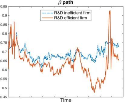
since risk loadings depend on those state variables. Existing empirical measures are limited to capture the time-series variant component of the risk loadings. Figure 1.7 presents the example of the beta path from the benchmark simulation for an innovation efficient firm and an innovation inefficient firm. Both firms have volatile risk loadings. Those volatile features of the real beta might generate the failure of empirical risk measures.
1.7
Testable Implications
In this section, I explore the empirical evidence that could support the theoretical work documented in the previous sections. The model suggests some testable implications. This section analyzes whether data corroborates the proposed mechanisms of the innovation ef-ficiency effect, operating leverage channel and output elasticity of physical capital channel (αk).
Data consists of the intersection of COMPUSTAT, CRSP, and NBER patent data. In-vestment analysis is based on yearly frequency data, and portfolio analysis uses monthly frequency data. Missing values on accounting data are converted to zero.
1.7.1
Operating leverage
In the previous section, simulation results imply that innovation efficiency intensifies the risk associated with operating leverage. Table 2.7 shows that innovation efficiency effect on stock returns is larger for high operating leverage firms. This section tests whether it is consistent with data. If the mechanism is valid, one should be able to find stronger innovation efficiency effect in high operating leverage firms.
The measure for analysis follows Gu, Hackbarth, and Johnson (2015). I run five-year rolling window regressions of operating costs on lagged operating costs, the current sale and lagged sale with quarterly data. By this rolling window regression, I can estimate how operating costs are associated with the current sale. The annual firm-level operating
leverage is the predicted operating costs when current sale is zero,11 scaled by current sale. As a predictor, I use annual mean values of lagged operating costs and lagged sale. Operating cost is the sum of costs of good sold and selling, general, and administrative expenses.12
Table 2.8 presents the results of 3-by-3 double sort portfolio analysis. Firms are sorted independently by operating leverage measure and innovation efficiency. The intersection of the two sorts forms the portfolio returns. Consistent with the model prediction, alpha and returns spread between high IE firms and low IE firms are large in high operating leverage portfolios. The spreads are from 0.44 to 0.85% per month when innovation efficiency is measured by citation scaled by R&D. The spread is the largest and significant in Fama-French 5 factor model. Within the same operating leverage portfolio, operating leverage does not vary much depending on innovation efficiency. When patent/R&D capital is used for innovation efficiency, the alpha or return spreads are large in high operating leverage portfolios as well.
1.7.2
Output elasticity of physical capital
Table 2.6 shows that innovation efficiency effect on stock returns is larger for high physical capital share to the profit (αk). If the mechanism is valid, then the innovation efficiency effect
should be larger in high capital share to profit firms. One problem is that it is unobservable variable. It might be associated with expansions option in a sense that firm can earn more profit with a dollar spent on physical capital. However, it is not solely about expansion option.
Even though an empirical measure equivalent to physical capital share in the model is not available, the model presents the consequences of high physical capital share. Figure 1.8 shows how firm values varies depending onαk. The slope of the line from the origin represents
the book-to-market ratio. Asαk increases, the book- to-market ratio decreases. It is natural
that firms making more sales with less capital should be valued more. Thus, they have the low book-to-market ratio. I assume that the book to market ratio capturesαk to some degree
11The predicted operating costs when the current sale is zero captures the intuition of “fixed costs”. 12The portfolio analysis with an alternative measure, operating cost scaled by sale, gives the similar results
and sort firms with the book-to-market ratio. Of course, it would be the perfect measure for capital share to sales, since the book-to-market ratio could capture many other things. However, it could be one of the necessary conditions for the validity of the mechanism that innovation efficiency effect is stronger in low book-to-market firms.
Table 1.10 presents the results of double sort portfolio analysis by the book-to-market ratio and innovation efficiency. Alpha and return spread between high IE firms and low IE firms are from 0.26 to 0.39 for low book-to-market firms while they are negligible for the high book to market firms. Average book to market ratios does not vary much in IE as long as firms fall in the same group of the book-to-market ratio. This means that book-to-market ratio does not play a role much for innovation efficiency effects. These results suggest that innovation efficiency effects are more associated with the low book-to-market firms and this might be related to the mechanisms of high capital share to profit implied in the model.
1.8
Conclusion
Following the framework of the investment-based model, I study the mechanism that gen-erates the innovation efficiency effect on stock returns; IE firms earn high subsequent stock returns. I analyze how innovation efficiency interacts with well-explored risk sources regard-ing investment. IE firms get riskier when they suffer high fixed costs. When they have more investment opportunities, IE firms take more risky projects. I found some empirical evidence that is consistent with the proposed mechanisms. The data shows that IE firms tend to invest more, which is implied by the model as well. Double sort portfolio analysis presents that innovation efficiency effect is stronger in high operating leverage firms and low book-to-market ratio firms.
This paper could be a good start of understanding how to value intangible knowledge capital, and how the knowledge capital intensive firms’ cost of equity should be measured. This paper stands in line with recent findings of the relationship between the operating environment and firm’s risk; features that increase firm value are not always decreasing equity risk loadings.
across firms exists in the economy. It just assumes that two different efficiencies of the firms exist and I analyze how the efficiency works for stock returns. Future work will need to incorporate how the efficiency heterogeneity are generated in the economy and how they evolve over time. Future work will need to address these points. With the augmented model, my model could be one of the useful tools to understand innovation activities under the neoclassical framework on the asset pricing side.
Besides, not only for asset pricing implication, my model might shed light on understand-ing the simultaneous dynamics of corporate investment policies and R&D policies. Model predictions of interactions between physical and knowledge capital can provide some testable implications. These predictions would stimulate future empirical research.
1.9
Figures and Tables
Figure 1.1: Investment and R&D policy
This figure represents the optimal policies of the physical capital-only firms and knowledge capital-only firms. k is physical capital, z is knowledge capital and x is aggregate productiv-ity. I/K is investment over physical capital and R/Z is R&D expenditures over knowledge capital. Panel (A) shows the optimal investment for the physical capital firms. Panel (B) depicts the R&D expenditures of the knowledge capital firms. Panel (C) compares the in-vestment and R&D expenditures when both firms are small (k and z are both 0.38) and panel (D) shows the comparison when they are large firms (k and z are 8.30).
Figure 1.2: R&D growth rate over the business cycle
This figure shows the COMPUSTAT weighted average R&D expenditures growth rate and real GDP growth rate. The sample for the R&D consists of all domestic observations in COMPUSTAT each year that reported positive R&D in both that year and the previous year. The weights are the lagged R&D expenditures and the sample is winsorized at 1% and 99% level. The grey area is recession.
Figure 1.3: Expected excess returns
Panel (A) shows the expected excess returns for the knowledge capital firms. After solving problems, conditional expectation can be implemented via matrix multiplication. Expected return is defined as Et[rt+1] ≡ Et[vt+1]/(vt − div.). ‘div’ is dividend. Expected excess
return is the expected returns minus risk free rate, rf ≡ 1/Et[mt+1]. Panel (B) plots the R&D expenditures-to-knowledge capital ratio as functions of knowledge capital z. I fix the aggregate productivity to long run mean. The arrows indicate the direction of the increase in innovation efficiencyζh. Firms withζh = 0.23 are plotted as crosses. Firms withζh = 0.25
Figure 1.4: Firm values.
This figure depicts the value function(v(k,z,x)). Panel (A) and (C) shows how firm value increases as physical and knowledge capital increases for innovation inefficient firm(ζh =
0.15), respectively. Panel (B) and (D) shows how firm value increases as physical and knowledge capital increases for innovation efficient firm(ζh = 0.45), respectively.
Figure 1.5: Optimal Policy functions.
This figure plots the optimal investment and R&D policies. IK is investment over physical capital and RK is R&D expenditure scaled by physical capital. Panel (A) and (C) are policy functions of innovation inefficient firms(ζh = 0.15). Panel (B) and (D)are policy functions
Figure 1.6: Innovation efficiency and Beta.
This figure shows the beta in equation (16). Panel (A) shows how beta as a function of physical capital changes when knowledge capital is fixed at the midpoint of its range. Panel (B) shows beta as a function of knowledge capital.
Figure 1.7: An example beta path
This figure shows the beta in equation (16). Panel (A) shows how beta as a function of physical capital changes when knowledge capital is fixed at the midpoint of its range. Panel (B) shows beta as a function of knowledge capital.
Figure 1.8: The book-to-market ratio and output elasticity of physical capital
Panel (A) plots values of the innovation inefficient firm. Panel (B) plots values of the innovation efficient firm depending on αk. The slope from the origin represents the inverse
Table 1.1: Fama-Macbeth (1973) regression of stock returns on innovative efficiency (in percent) from Hirshleifer, Hsu, and Li (2013).
This table presents the result of Fama-Macbeth(1973) regressions from Hirshleifer, Hsu, and Li (2013). IE stands for innovation efficiency. RDC is the 5-year cumulative R&D expenditures with a depreciation rate of 20%. RD is R&D expenditures. BTM is book to market ratio. CapEX is capital expenditures. ME is market equity. The sample period is from 1976 -2006. The sample consists of the intersection of CRSP, Compustat, IBES, and NBER patent database. Finance, insurance,and real estate sectors are dropped in the sample. IE = citations/RD IE = patents/RDC ln(1+IE) 0.11 0.07 0.08 0.04 (5.13) (2.92) (4.44) (1.81) ln(1+RD/ME) 0.13 0.13 (3.22) (3.28) ln(Size) -0.30 -0.30 -0.30 -0.30 (-3.13) (-3.14) (-3.06) (-3.13) ln(BTM) 0.39 0.37 0.39 0.37 (6.73) (6.34) (6.76) (6.32) ln(1+CapEx/ME) -0.11 -0.12 -0.11 -0.12 (-3.09) (-3.25) (-3.09) (-3.25) ROA 0.15 0.15 0.15 0.16 (2.93) (3.16) (2.96) (3.20)
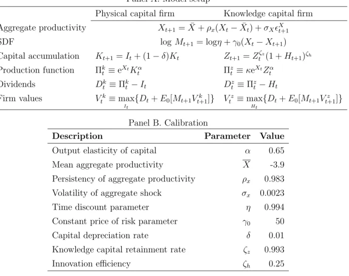
Table 1.2: Simple models and calibration
This table presents the model setup of physical capital firms and knowledge capital firms. Panel A. Model setup
Physical capital firm Knowledge capital firm Aggregate productivity Xt+1 = ¯X+ρx(Xt−X¯t) +σXXt+1 SDF log Mt+1 = logη+γ0(Xt−Xt+1) Capital accumulation Kt+1 =It+ (1−δ)Kt Zt+1 =Ztζz(1 +Ht+1)ζh Production function Πk t ≡eXtKtα Πzt ≡κeXtZtα Dividends Dkt ≡Πkt −It Dzt ≡Πzt −Ht
Firm values Vtk ≡max
It
{Dt+E0[Mt+1Vtk+1]} Vtz ≡max
Ht
{Dt+E0[Mt+1Vtz+1]} Panel B. Calibration
Description Parameter Value
Output elasticity of capital α 0.65
Mean aggregate productivity X -3.9
Persistency of aggregate productivity ρx 0.983
Volatility of aggregate shock σx 0.0023
Time discount parameter η 0.994
Constant price of risk parameter γ0 50
Capital depreciation rate δ 0.01
Knowledge capital retainment rate ζz 0.993
Table 1.3: Innovation efficiency and investment.
This table presents the panel regression coefficients(in percent) and their t-statistics of phys-ical capital investment on innovation efficiency. Sample period is from 1977 to 2006, and consists of COMPUSTAT, CRSP, and NBER patent data. IE stands for innovation efficiency, measured by patents number granted divided by R&D capital and by number of citations scaled by past cumulative R&D expenditures. CAPX is capital expenditures. AT is total asset. Size is market equity on December in year t-1. ROA is income before extraordinary items plus interest and related expense divided by lagged total asset, (ibt+xintt)/att−1. AG is asset growth rate, (att−att−1)/att. NS is net stock issues, log(shoutt/shoutt−1). AD is advertising expense. shout is split adjusted share outstanding. expense(compustat item xad). Fama-French 48 industry code is used for controlling for industry fixed effect. All variables are winsorized at the 1% and 99% level and normalized to mean 0 and standard deviation 1. log(1+CAPX/AT) patents/RDC citation/RD log(1+IE) 0.1490 0.1511 0.1572 0.1580 (3.91) (3.97) (3.72) (3.72) log(BE/ME) -0.4927 -0.5048 -0.4684 -0.4889 (-10.23) (-10.43) (-9.40) (-9.85) Size 0.6433 0.6004 0.6847 0.6158 (11.55) (10.53) (12.05) (10.59) log(1+RD/ME) 0.1349 0.1803 0.1159 0.1917 (4.18) (5.25) (3.52) (5.48) ROA 0.0876 0.1547 (2.13) (3.27) AG 0.1222 0.2611 (2.98) (4.92) NS -0.1026 -0.1594 (-2.74) (-3.41) log(1+AD/ME) -0.1519 -0.1888 (-3.32) (-4.15)
year FE Yes Yes Yes Yes
Table 1.4: Calibration.
This table summarizes the calibration for the benchmark model. innovation efficiency in parenthesis is for the innovation efficient firm.
Description Parameter Value
Physical capital share αk 0.6
Knowledge capital share αz 0.3
Mean aggregate productivity x -3.2
Persistency of aggregate productivity ρx 0.983
Volatility of aggregate shock σx 0.0023
Volatility of R&D σν 0.01
Time discount parameter η 0.994
Proportional cost f 0.01
Constant price of risk parameter γ0 50
Time-varying price of risk parameter γ1 -1000
Capital depreciation rate δ 0.01
Capital adjustment cost a 15
Fixed equity issuance cost λ0 0.08
Proportional equity issuance cost λ1 0.025 Knowledge capital retainment rate ζz 0.993
Table 1.5: Unconditional moments of the simulated panel.
Risk free rate and standard deviation of risk free rate are from Campbell, Lo, and Mackinlay, 1997. The average investment to book asset is from Abel and Eberly (2001). Volatility of Investment to book asset is from Hennessy, and Whited, 2005. The average book to market ratio is from Pontiff, and Schall 1998. The rest are from Chan, Lakonishock, and Sougianni, 2001. innovation inefficient firms has the ζh = 0.15 and innovation efficient firms
has ζh = 0.45. Return on equity in simulated data is calculated as (ki,t+1−ki,t+di,t)/ki,t.
Data Inef. firms Ef. firms The annual average risk free rate 0.018 0.019 0.019 The volatility of annual risk free rate 0.030 0.023 0.023 The average annual investment to book assets ratio 0.150 0.119 0.125 The volatility of annual investment to book assets ratio 0.077 0.006 0.025 The average annual R&D to book assets ratio 0.076 0.039 0.115 The average annual R&D to market value ratio 0.058 0.046 0.041 The average book to market ratio 0.668 1.118 0.439 The average return on equity(profitability) 0.088 0.184 0.137
Table 1.6: Fama-Macbeth regression results from the simulated data
This table presents Fama-Macbeth(1973) regression results with the simulated data. The dependent variable is excess return. 1000 panels are simulated. Each panel has 5000 firms and 720 months. First 240 months are dropped. For each panel Fama-Macbeth regression is implemented. The coefficients and t-statistics are cross panel averages. EFF is a dummy variable that gives one when ζh = 0.45 and gives zero otherwise. RK is R&D expenditures
scaled by physical capital. BEME is book to market ratio. Profitability is defined as(ki,t+1−
ki,t + di,t)/ki,t. IK is investment to book value ratio. Size is log of market value. All
independent variables except dummy variables are normalized and winsorized at 1% and 99% level. (1) (2) (3) (4) EFF 0.0008 0.0231 0.0165 0.0132 (1.20) (9.13) (7.71) (5.43) RK 0.0164 (2.38) BEME 0.0134 0.0091 0.0034 (12.73) (5.81) (3.10) Prof. 0.0020 (-0.33) IK -0.0006 (0.38) Size -0.0194 -0.0124 -0.0114 (-12.39) (-9.72) (-7.76) Const. 0.0132 -0.0021 0.0039 0.0101 (4.24) (-0.77) (1.35) (2.12)
Table 1.7: Monthly Fama-Macbeth regression: homogenous panel.
This table presents Fama-Macbeth(1973) regression results with the simulated data. Panel A is simulated with innovation inefficient firms (ζh =0.15)and Panel B is simulated with the
innovation efficient firms (ζh =0.45) The dependent variable is excess return. 1000 panels are
simulated. Each panel has 5000 firms and 720 months. First 240 months are dropped. For each panel Fama-Macbeth regression is implemented. All independent variables are defined as in table 4. Panel A: ζh =0.15 (1) (2) (3) (4) (5) (6) RK 0.0032 0.0023 0.0025 0.0029 0.0006 0.0007 (12.36) (11.09) (11.32) (12.69) (2.86) (2.29) BEME 0.0138 0.0158 (6.90) (4.60) Prof. -0.0009 (-7.96) IK -0.0007 (-2.37) Size -0.0066 -0.0051 (-11.03) (-10.36) cons. 0.0186 0.0192 0.0187 0.0191 0.0187 0.0195 (5.27) (5.42) (5.26) (5.27) (5.02) (5.25) Panel B: ζh =0.45 (1) (2) (3) (4) (5) (6) RK 0.0012 0.0014 0.0023 0.0006 0.0006 0.0004 (6.72) (7.53) (2.73) (2.51) (7.54) (7.09) BEME 0.0003 0.0019 (0.10) (1.70) Profit. 0.0004 (0.44) IK -0.0007 (0.07) Size -0.0016 -0.0035 (-1.50) (-2.40) cons. 0.0085 0.0080 0.0084 0.0079 0.0075 0.0102 (2.54) (2.31) (2.52) (2.15) (2.07) (2.53)
Table 1.8: FM regression results from the alternative parametrization.
This table presents the Fama-Macbeth (1973) regression results with alternative parame-trezation. 1000 panels are simulated. Each panel has 2500 innovation efficient firms and 2500 innovation inefficient firms are simulated for 720 months and firs 240 months are dropped. Independent variables are defined the same as in the table 3. Column (1) is benchmark calibration. I set alternative parameters such as zero proportional cost f = 0 in column (2), low capital share αk = 0.55 in column (3). high capital share αk = 0.65 column (4),
constant sharp ratio γ1 = 0 in column (5), low sharp ratio γ0 = 30 in column(6), and low capital adjustment cost a= 0 in column (7).
BM f = 0 αk = 0.55 αk = 0.65 γ1 = 0 γ0 = 30 a = 0 EFF 0.0132 0.0023 0.0025 0.0193 0.0157 0.0054 0.0150 (5.43) (2.74) (3.44) (7.25) (5.54) (8.77) (4.44) RK 0.0164 0.0003 0.0083 0.0029 0.0031 -0.0004 0.0067 (2.38) (1.17) (1.48) (1.34) (2.24) (-2.84) (3.47) BEME 0.0034 0.0020 0.0474 0.0011 0.0014 0.0018 0.0021 (3.10) (4.45) (4.73) (2.52) (2.34) (5.27) (4.23) Prof. 0.0020 0.0001 0.0040 0.0001 0.0008 0.0004 -0.0002 -(0.33) (-0.35) (2.15) (-1.19) (0.10) (1.89) (-0.40) IK -0.0006 0.0014 -0.0025 -0.0002 -0.0012 -0.0002 -0.0064 (0.38) (1.90) (-0.24) (0.41) (-0.20) (-0.64) (-0.95) Size -0.0114 -0.0031 -0.0087 -0.0148 -0.0146 -0.0063 -0.0119 (-7.76) (-3.53) (-7.79) (-8.11) (-6.63) (-12.01) (-6.55) Const. 0.0101 0.0092 0.0141 0.0029 0.0066 0.0086 0.0062 (2.12) (1.71) (3.34) (0.97) (1.12) (3.99) (1.40)