BNSP: an R Package for Fitting Bayesian Semiparametric
Regression Models and Variable Selection
Georgios Papageorgiou
Department of Economics, Mathematics and Statistics
Birkbeck, University of London, UK
[email protected]
Abstract
The R package BNSP provides a unified framework for semiparametric location-scale regression and stochastic search variable selection. The statistical methodology that the package is built upon utilizes basis function expansions to represent semiparametric covariate effects in the mean and variance functions, and spike-slab priors to perform selection and regularization of the estimated effects. In addition to the main function that performs posterior sampling, the package includes functions for assessing convergence of the sampler, summarizing model fits, visualizing covariate effects and obtaining predictions for new responses or their means given feature/covariate vectors.
Keywords: additive models; basis functions; heteroscedastic models; variable selection
1
Introduction
There are many approaches to non- and semi-parametric modeling. From a Bayesian perspective, M¨uller & Mitra (2013) provide a review that covers methods for density estimation, modeling of random effects distributions in mixed effects models, clustering and modeling of unknown functions in regression models. Our interest is on Bayesian methods for modeling unknown functions in regression models. In particular, we are interested in modeling both the mean and variance functions non-parametrically, as general functions of the covariates. There are multiple reasons why allowing the variance function to be a general function of the covariates may be important (Chan et al., 2006). Firstly, it can result in more realistic prediction intervals than those obtained by assuming constant error variance, or as M¨uller & Mitra (2013) put it, it can result in more honest representation of uncertainties. Secondly, it allows the practitioner to examine and understand which covariates drive the variance. Thirdly, it results in more efficient estimation of the mean function, and lastly, it produces more accurate standard errors of unknown parameters.
In the R (R Core Team, 2016) packageBNSP (Papageorgiou, 2018) we implemented Bayesian regres-sion models with Gaussian errors and with mean and log-variance functions that can be modeled as general functions of the covariates. Covariate effects may enter the mean and log-variance functions parametri-cally or non-parametriparametri-cally, with the nonparametric effects represented as linear combinations of basis functions. The strategy that we follow in representing unknown functions is to utilize a large number of basis functions. This allows for flexible estimation and for capturing true effects that are locally adaptive. Potential problems associated with large numbers of basis functions, such as over-fitting, are avoided in our
implementation, and efficient estimation is achieved, by utilizing spike-slab priors for variable selection. A review of variable selection methods is provided by O’Hara & Sillanp¨a¨a (2009).
The methods described here belong to the general class of models known as generalized additive models for location, scale and shape (GAMLSS) (Rigby & Stasinopoulos, 2005; Stasinopoulos & Rigby, 2007) or the Bayesian analogue termed as BAMLSS (Umlauf et al., 2018) and implemented in package bamlss (Umlauf et al., 2017). However, due to the nature of the spike-and-slab priors that we have implemented, in addition to flexible modeling of the mean and variance functions, the methods described here can also be utilized for selecting promising subsets of predictor variables in multiple regression models. The implemented methods fall in the general class of methods known as stochastic search variable selection (SSVS). SSVS has received considerable attention in the Bayesian literature and its applications range from investigating factors that affect individual’s happiness (George & McCulloch, 1993), to constructing financial indexes (George & McCulloch, 1997) and to gene mapping (O’Hara & Sillanp¨a¨a, 2009). These methods associate each regression coefficient, either a main effect or the coefficient of a basis function, with a latent binary variable that indicates whether the corresponding covariate is needed in the model or not. Hence, the joint posterior distribution of the vector of these binary variables can identify the models with the higher posterior probability.
R packages that are related to BNSP include spikeSlabGAM (Scheipl, 2016) that also utilizes SSVS methods (Scheipl, 2011). A major difference between the two packages, however, is that whereas spikeSlabGAM utilizes spike-and-slab priors for function selection, BNSP utilizes spike-and-slab priors for variable selection. In addition, Bayesian GAMLSS models, also refer to as distributional regression models, can also be fit with R package brms using normal priors (B¨urkner, 2018). Further, the R pack-age gamboostLSS (Hofner et al., 2018) includes frequentist GAMLSS implementation based on boosting that can handle high-dimensional data (Mayr et al., 2012). Lastly, the R package mgcv (Wood, 2018) can also fit generalized additive models with Gaussian errors and integrated smoothness estimation, with implementations that can handle large datasets.
InBNSP we have implemented functions for fitting such semi-parametric models, summarizing model fits, visualizing covariate effects and predicting new responses or their means. The main functions are
mvrm, mvrm2mcmc, print.mvrm, summary.mvrm, plot.mvrm andpredict.mvrm. A quick description of these functions follows. The first one, mvrm, returns samples from the posterior distributions of the model parameters, and it is based on an efficient Markov chain Monte Carlo (MCMC) algorithm in which we integrate out the coefficients in the mean function, generate the variable selection indicators in blocks (Chan et al., 2006) and choose the MCMC tuning parameters adaptively (Roberts & Rosenthal, 2009). In order to minimize random-access memory utilization, posterior samples are not kept in memory, but instead written in files in a directory supplied by the user. The second function, mvrm2mcmc, reads-in the samples from the posterior of the model parameters and it creates an object of class"mcmc". This enables users to easily utilize functions from package coda (Plummer et al., 2006), including functions plot and summary
for assessing convergence and for summarizing posterior distributions. Further, functions print.mvrmand
summary.mvrm provide summaries of model fits, including models and priors specified, marginal posterior probabilities of term inclusion in the mean and variance models and models with the highest posterior probabilities. Function plot.mvrm creates plots of parametric and nonparametric terms that appear in the mean and variance models. The function can create two-dimensional plots by calling functions from package ggplot2 (Wickham, 2009). It can also create static or interactive three-dimensional plots by calling functions from packages plot3D (Soetaert, 2016) and threejs (Lewis, 2016). Lastly, function
predict.mvrmprovides predictions either for new responses or their means given feature/covariate vectors. We next provide a detailed model description followed by illustrations on the usage of the package and the options it provides. Technical details on the implementation of the MCMC algorithm are provided in the Appendix. The paper concludes with a brief summary.
2
Mean-variance nonparametric regression models
Let y = (y1, . . . , yn)> denote the vector of responses and let X = [x1, . . . ,xn]> and Z = [z1, . . . ,zn]>
denote design matrices. The models that we consider express the vector of responses utilizing
Y =β01n+Xβ1 +,
where 1n is the usual n-dimensional vector of ones, β0 is an intercept term, β1 is a vector of regression
coefficients and = (1, . . . , n)> is an n-dimensional vector of independent random errors. Each i, i =
1, . . . , n,is assumed to have a normal distribution, i ∼N(0, σi2), with variances that are modeled in terms
of covariates. Let σ2 = (σ2
1, . . . , σn2)
>. We model the vector of variances utilizing log(σ2) =α01n+Zα1,
where α0 is an intercept term and α1 is a vector of regression coefficients. Equivalently, the model for the
variances can be expressed as
σ2i =σ2exp(z>i α1), i= 1, . . . , n, (1)
where σ2 = exp(α 0).
Let D(α) denote an n-dimensional, diagonal matrix with elements exp(z>i α1/2), i = 1, . . . , n. Then,
the model that we consider may be expressed more economically as
Y =X∗β+,
∼N(0, σ2D2(α)), (2)
where β = (β0,β>1)> and X
∗
= [1n,X].
In the next subsections we describe how, within model (2), both parametric and nonparametric effects of explanatory variables on the mean and variance functions can be captured utilizing regression splines and variable selection methods. We begin by considering the special case where there is a single covariate entering the mean model and a single covariate entering the variance model.
2.1
Locally adaptive models with a single covariate
Suppose that the observed dataset consists of triplets (yi, ui, wi), i= 1, . . . , n,where explanatory variables
u and w enter flexibly the mean and variance models, respectively. To model the nonparametric effects of u and w we consider the following formulations of the mean and variance models
µi =β0+fµ(ui) =β0+ q1 X j=1 βjφ1j(ui) = β0+x>i β1, (3) log(σi2) = α0+fσ(wi) =α0+ q2 X j=1 αjφ2j(wi) =α0+z>i α1. (4) In the preceding xi = (φ11(ui), . . . , φ1q1(ui)) > and z i = (φ21(wi), . . . , φ2q2(wi))
> are vectors of basis func-tions and β1 = (β1, . . . , βq1)
> and α
1 = (α1, . . . , αq2)
> are the corresponding coefficients.
In package BNSP we implemented two sets of basis functions. Firstly, radial basis functions
B1 =
φ1(u) = u, φ2(u) =||u−ξ1||2log ||u−ξ1||2
, . . . , φq(u) =||u−ξq−1||2log ||u−ξq−1||2
where ||u||denotes the Euclidean norm of uand ξ1, . . . , ξq−1 are the knots that within package BNSPare
chosen as the quantiles of the observed values of explanatory variableu, withξ1 = min(ui),ξq−1 = max(ui)
and the remaining knots chosen as equally spaced quantiles between ξ1 and ξq−1.
Secondly, we implemented thin plate splines
B2 ={φ1(u) =u, φ2(u) = (u−ξ1)+, . . . , φq(u) = (u−ξq)+},
where (a)+ = max(a,0) and the knots ξ1, . . . , ξq−1 are determined as above.
In addition,BNSPsupports the smooth constructors from packagemgcve.g. the low-rank thin plate splines, cubic regression splines, P-splines, their cyclic versions and others. Examples on how these smooth terms are used within BNSP are provided later in this paper.
Locally adaptive models for the mean and variance functions are obtained utilizing the methodology developed by Chan et al. (2006). Considering the mean function, local adaptivity is achieved by utilizing a large number of basis functions q1. Over-fitting, and problems associated with it, is avoided by allowing
positive prior probability that the regression coefficients are exactly zero. The latter is achieved by defining binary variables γj, j = 1, . . . , q1, that take valueγj = 1 ifβj 6= 0 andγj = 0 if βj = 0. Hence, vector γ =
(γ1, . . . , γq1)
> determines which terms enter the mean model. The vector of indicators δ = (δ
1, . . . , δq2)
> for the variance function is defined analogously.
Given vectorsγ and δ, the heteroscedastic, semiparametric model (2) can be written as
Y =X∗γβγ+,
∼N(0, σ2D2(αδ)),
where βγ consisting of all non-zero elements of β1 and X∗γ consists of the corresponding columns of X∗. Subvector αδ is defined analogously.
We note that, as was suggested by Chan et al. (2006), we work with mean corrected columns in the design matrices X and Z, both in this paper and in the BNSP implementation. We remove the mean from all columns in the design matrices except those that correspond to categorical variables.
2.2
Prior specification for models with a single covariate
Let ˜X =D(α)−1X∗
. The prior for βγ is specified as (Zellner, 1986)
βγ|cβ, σ2,γ,α,δ ∼N(0, cβσ2( ˜X
>
γX˜γ)−1).
Further, the prior forαδ is specified as
αδ|cα,δ ∼N(0, cαI).
Independent priors are specified for the indicators variables γj as P(γj = 1|πµ) = πµ, j = 1, . . . , q1,
from which the joint prior is obtained as
P(γ|πµ) =πµN(γ)(1−πµ)q1−N(γ),
where N(γ) = Pq1 j=1γj.
Similarly, for the indicatorsδj we specify independent priorsP(δj = 1|πσ) =πσ, j = 1, . . . , q2. It follows
that the joint prior is
where N(δ) = Pq2 j=1δj.
We specify inverse Gamma priors forcβ and cα and Beta priors forπµ and πσ
cβ ∼IG(aβ, bβ), cα∼IG(aα, bα),
πµ∼Beta(cµ, dµ), πσ ∼Beta(cσ, dσ). (6)
Lastly, for σ2 we consider inverse Gamma and half-normal priors
σ2 ∼IG(aσ, bσ) andσ∼N(σ; 0, φ2σ)I[σ >0]. (7)
2.3
Extension to bivariate covariates
It is straightforward to extend the methodology described earlier to allow fitting of flexible mean and variance surfaces. In fact, the only modification required is in the basis functions and knots. For fitting surfaces, in package BNSP we implemented radial basis functions
B3 = n φ1(u) = u1, φ2(u) = u2, φ3(u) = ||u−ξ1|| 2log ||u−ξ 1|| 2 , . . . , φq(u) =||u−ξq−2|| 2log ||u−ξ q−2|| 2o .
We note that the prior specification presented earlier for fitting flexible functions remains unchained for fitting flexible surfaces. Further, for fitting bivariate or higher order functions, BNSP also supports smooth constructors s, te and ti frommgcv.
2.4
Extension to additive models
In the presence of multiple covariates, the effects of which may be modeled parametrically or semipara-metrically, the mean model in (3) is extended to the following
µi =β0+u>ipβ+
K1
X
k=1
fµ,k(uik), i= 1, . . . , n,
where, uip includes the covariates the effects of which are modeled parametrically, β denotes the
corre-sponding effects, and fµ,k(uik), k = 1, . . . , K1, are flexible functions of one or more covariates expressed
as fµ,k(uik) = q1k X j=1 βkjφ1kj(uik),
where φ1kj, j = 1, . . . , q1k are the basis functions used in the kth component, k = 1, . . . , K1.
Similarly, the variance model (4), in the presence of multiple covariates, is expressed as
log(σ2i) = α0+w>ipα+ K2 X k=1 fσ,k(wik), i= 1, . . . , n, where fσ,k(wik) = q2k X j=1 αkjφ2kj(wik).
For additive models, local adaptivity is achieved using a similar strategy as in the single covariate case. That is, we utilize a potentially large number of knots or basis functions in the flexible components that appear in the mean model, fµ,k, k = 1, . . . , K1, and in the variance model, fσ,k, k = 1, . . . , K2.
To avoid over-fitting, we allow removal of the unnecessary ones utilizing the usual indicator variables,
γk = (γk1, . . . , γkq1k)
>, k = 1, . . . , K
1, and δk = (δk1, . . . , δkq2k)
>, k = 1, . . . , K
2. Here, vectors γk and δk
determine which basis functions appear in fµ,k and fσ,k respectively.
The model that we implemented in package BNSP specifies independent priors for the indicators variables γkj asP(γkj = 1|πµk) = πµk, j = 1, . . . , q1k. From these, the joint prior follows
P(γk|πµk) =π N(γk) µk (1−πµk) q1k−N(γk), where N(γk) = Pq1k j=1γkj.
Similarly, for the indicators δkj we specify independent priors P(δkj = 1|πσk) = πσk, j = 1, . . . , q2k. It
follows that the joint prior is
P(δk|πσk) =π
N(δk)
σk (1−πσk)
q2k−N(δk),
where N(δk) = Pqj2=1k δkj.
We specify the following independent priors for the inclusion probabilities.
πµk ∼Beta(cµk, dµk), k = 1, . . . , K1 πσk ∼Beta(cσk, dσk), k= 1, . . . , K2. (8)
The rest of the priors are the same as those specified for the single covariate models.
3
Usage
In this section we provide results on simulation studies and real data analyses. The purpose is twofold: firstly we point out that the package works well and provides the expected results (in simulation studies) and secondly we illustrate the options that the users of BNSP have.
3.1
Simulation studies
Here we present results from three simulations studies, involving one, two, and multiple covariates. For the majority of these simulation studies, we utilize the same data-generating mechanisms as those presented by Chan et al. (2006).
3.1.1 Single covariate case
We consider two mechanisms that involve a single covariate that appears in both the mean and vari-ance model. Denoting the covariate by u, the data-generating mechanisms are the normal model Y ∼
N{µ(u), σ2(u)} with the following mean and standard deviation functions 1. µ(u) = 2u, σ(u) = 0.1 +u,
2. µ(u) ={N(u, µ= 0.2, σ2 = 0.004) +N(u, µ= 0.6, σ2 = 0.1)}/4,
σ(u) ={N(u, µ= 0.2, σ2 = 0.004) +N(u, µ= 0.6, σ2 = 0.1)}/6.
We generate a single dataset of size n = 500 from each mechanism, where variable u is obtained from the uniform distribution, u∼Unif(0,1). For instance, for obtaining a dataset from the first mechanism we use
> mu <- function(u){2 * u} > stdev <- function(u){0.1 + u} > set.seed(1) > n <- 500 > u <- sort(runif(n)) > y <- rnorm(n,mu(u),stdev(u)) > data <- data.frame(y,u)
Above we specified the seed value to be one, and we do so in what follows, so that our results are replicable. To the generated dataset we fit a special case of the model that we presented, where the mean and variance functions in (3) and (4) are specified as
µ=β0+fµ(u) =β0+
q1
X
j=1
βjφ1j(u) and log(σ2) =α0 +fσ(u) = α0+
q2
X
j=1
αjφ2j(u), (9)
withφ denoting the radial basis functions presented in (5). Further, we chooseq1 =q2 = 21 basis functions
or, equivalently, 20 knots. Hence, we have φ1j(u) =φ2j(u), j = 1, . . . ,21, which results in identical design
matrices for the mean and variance models. In R, the two models are specified using
> model <- y ~ sm(u, k = 20, bs = "rd") | sm(u, k = 20, bs = "rd")
The above formula (Zeileis & Croissant, 2010) specifies the response, mean and variance models. Smooth terms are specified utilizing function sm, that takes as input the covariateu, the selected number of knots and the selected type of basis functions.
Next we specify the hyper-parameter values for the priors in (6) and (7). The default prior for cβ is
inverse Gamma with aβ = 0.5, bβ = n/2 (Liang et al., 2008). For parameter cα the default prior is a
non-informative but proper inverse Gamma with aα =bα = 1.1. Concerning πµ and πσ, the default priors
are uniform, obtained by setting cµ = dµ = 1 and cσ = dσ = 1. Lastly, the default prior for the error
standard deviation is the half-normal with variance φ2
σ = 2, |σ| ∼N(0,2).
We choose to run the MCMC sampler for 10,000 iterations and discard the first 5,000 as burn-in. Of the remaining 5,000 samples we retain 1 every 2 samples, resulting in 2,500 posterior samples. Further, as mentioned above, we set the seed of the MCMC sampler equal to one. Obtaining posterior samples is achieved by a function call of the form
> m1 <- mvrm(formula = model, data = data, sweeps = 10000, burn = 5000,
+ thin = 2, seed = 1, StorageDir = DIR,
+ c.betaPrior = "IG(0.5,0.5*n)", c.alphaPrior = "IG(1.1,1.1)",
+ pi.muPrior = "Beta(1,1)", pi.sigmaPrior = "Beta(1,1)", sigmaPrior = "HN(2)")
Samples from the posteriors of the model parameters {β,γ,α,δ, cβ, cα, σ2} are written in seven separate
files which are stored in the directory specified by argument StorageDir. If a storage directory is not specified, then function mvrm returns an error message, as without these files there will be no output to process. Furthermore, the last two lines of the above function call show the specified priors, which are cβ ∼ IG(0.5, n/2), cα ∼ IG(1.1,1.1), πµ ∼ Beta(1,1), πσ ∼Beta(1,1) and |σ| ∼ N(0,2), respectively. As
we mentioned above, these priors are the default ones, and hence the same function call can be achieved without specifying the last two lines. Here we display the priors in order to describe how users can specify their own priors. For parameters cβ and cα only inverse Gamma priors are available, with parameters that
in function mvrm by using c.betaPrior = "IG(1.01,1.01)". The second parameter of the prior for cβ
can be a function of the sample size n (but only symbol n would work here), so for instancec.betaPrior = "IG(1,0.4*n)" is another acceptable specification. Further, Beta priors are available for parametersπµ
and πσ with parameters that can be specified by the user again in the intuitive way. Lastly, two priors are
available for the error variance. These are the default half-normal and the inverse Gamma. For instance,
sigmaPrior = "HN(5)" defines |σ| ∼ N(0,5) as the prior while sigmaPrior = "IG(1.1,1.1)" defines σ2 ∼IG(1.1,1.1) as the prior.
Functionmvrm2mcmc reads in posterior samples from the files that the call to function mvrmgenerated and creates an object of class "mcmc". Hence, for summarizing posterior distributions and for assessing convergence, functions summary and plot from package coda can be used. As an example, here we read in the samples from the posterior of β
> beta <- mvrm2mcmc(m1, "beta")
and summarize the posterior using summary. For the sake of economizing space, only the part of the output that describes the posteriors of β0, β1, and β2 is shown below
> summary(beta)
Iterations = 5001:9999 Thinning interval = 2 Number of chains = 1
Sample size per chain = 2500
1. Empirical mean and standard deviation for each variable, plus standard error of the mean:
Mean SD Naive SE Time-series SE
(Intercept) 9.534e-01 0.004399 8.799e-05 0.0002534
u 1.864e+00 0.042045 8.409e-04 0.0010356
sm(u).1 3.842e-04 0.016421 3.284e-04 0.0003284
2. Quantiles for each variable:
2.5% 25% 50% 75% 97.5%
(Intercept) 0.946 0.9513 0.9533 0.9554 0.960
u 1.833 1.8565 1.8614 1.8682 1.923
sm(u).1 0.000 0.0000 0.0000 0.0000 0.000
Further, we may obtain a plot using
> plot(beta)
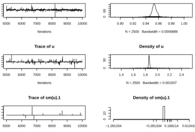
Figure 1 shows the first three of the plots created by function plot. These are the plots of the samples from the posteriors of coefficients β0, β1 and β2. As we can see from both the summary and Figure 1, only
the first two coefficients have posteriors that are not centered around zero.
Returning to function mvrm2mcmc, it requires two inputs. These are an object of class "mvrm" and the name of the file to be read in R. For the parameters in the current model {β,γ,α,δ, cβ, cα, σ2} the
5000 6000 7000 8000 9000 10000 0.90 1.00 Iterations Trace of (Intercept) 0.90 0.92 0.94 0.96 0.98 1.00 0 60 Density of (Intercept) N = 2500 Bandwidth = 0.0006888 5000 6000 7000 8000 9000 10000 1.4 2.2 Iterations Trace of u 1.4 1.6 1.8 2.0 2.2 2.4 0 30 Density of u N = 2500 Bandwidth = 0.001937 5000 6000 7000 8000 9000 10000 −0.2 0.4 Iterations
Trace of sm(u).1 Density of sm(u).1
0
10
−1.281334 −0.281334 0.168114 0.613418
Figure 1: Trace and density plots for the regression coefficientsβ0, β1andβ2 of the first simulated example.
Parameters β1 and β2 are the coefficients of the first two basis functions, denoted by ‘u’ and ‘sm(u).1’.
Plots for coefficients β3, . . . , β21 are omitted as they follow a very similar pattern to that seen for β2 i.e.
most of the time they take value zero but with random spikes away from zero.
Summaries of ‘mvrm’ fits may be obtained utilizing functionsprint.mvrmandsummary.mvrm. Function
print takes as input an object of class "mvrm". It returns basic information at the model fit as shown below
> print(m1) Call:
mvrm(formula = model, data = data, sweeps = 10000, burn = 5000,
thin = 2, seed = 1, StorageDir = DIR, c.betaPrior = "IG(0.5,0.5*n)", c.alphaPrior = "IG(1.1,1.1)", pi.muPrior = "Beta(1,1)",
pi.sigmaPrior = "Beta(1,1)", sigmaPrior = "HN(2)") 2500 posterior samples
Mean model - marginal inclusion probabilities
u sm(u).1 sm(u).2 sm(u).3 sm(u).4 sm(u).5 sm(u).6 sm(u).7
1.0000 0.0040 0.0036 0.0032 0.0084 0.0036 0.0044 0.0028
sm(u).8 sm(u).9 sm(u).10 sm(u).11 sm(u).12 sm(u).13 sm(u).14 sm(u).15
0.0060 0.0020 0.0060 0.0036 0.0056 0.0056 0.0036 0.0052
sm(u).16 sm(u).17 sm(u).18 sm(u).19 sm(u).20
0.0060 0.0044 0.0056 0.0044 0.0052
Variance model - marginal inclusion probabilities
u sm(u).1 sm(u).2 sm(u).3 sm(u).4 sm(u).5 sm(u).6 sm(u).7
1.0000 0.6072 0.5164 0.5808 0.5488 0.6760 0.5320 0.6336
0.6936 0.6708 0.5996 0.4816 0.4912 0.3728 0.6268 0.5688 sm(u).16 sm(u).17 sm(u).18 sm(u).19 sm(u).20
0.5872 0.6528 0.4428 0.6900 0.5356
The function returns a matched call, the number of posterior samples obtained and marginal inclusion probabilities of the terms in the mean and variance models.
Whereas the output of functionprintfocuses on marginal inclusion probabilities, the output of function
summaryfocuses on the most frequently visited models. It takes as input an object of class ‘mvrm’ and the number of (most frequently visited) models to be displayed, which by default is set to nModels = 5. Here to economize space we set nModels = 2. The information returned by functions summaryis shown below
> summary(m1, nModels = 2)
Specified model for the mean and variance:
y ~ sm(u, k = 20, bs = "rd") | sm(u, k = 20, bs = "rd") Specified priors:
[1] c.beta = IG(0.5,0.5*n) c.alpha = IG(1.1,1.1) pi.mu = Beta(1,1)
[4] pi.sigma = Beta(1,1) sigma = HN(2)
Total posterior samples: 2500 ; burn-in: 5000 ; thinning: 2 Files stored in /home/papgeo/1/
Null deviance: 1299.292
Mean posterior deviance: -88.691
Joint mean/variance model posterior probabilities:
mean.u mean.sm.u..1 mean.sm.u..2 mean.sm.u..3 mean.sm.u..4 mean.sm.u..5
1 1 0 0 0 0 0
2 1 0 0 0 0 0
mean.sm.u..6 mean.sm.u..7 mean.sm.u..8 mean.sm.u..9 mean.sm.u..10
1 0 0 0 0 0
2 0 0 0 0 0
mean.sm.u..11 mean.sm.u..12 mean.sm.u..13 mean.sm.u..14 mean.sm.u..15
1 0 0 0 0 0
2 0 0 0 0 0
mean.sm.u..16 mean.sm.u..17 mean.sm.u..18 mean.sm.u..19 mean.sm.u..20 var.u
1 0 0 0 0 0 1
2 0 0 0 0 0 1
var.sm.u..1 var.sm.u..2 var.sm.u..3 var.sm.u..4 var.sm.u..5 var.sm.u..6
1 1 1 1 1 1 1
2 1 0 1 1 1 1
var.sm.u..7 var.sm.u..8 var.sm.u..9 var.sm.u..10 var.sm.u..11 var.sm.u..12
1 1 1 1 0 1 0
2 1 1 1 1 1 1
var.sm.u..13 var.sm.u..14 var.sm.u..15 var.sm.u..16 var.sm.u..17 var.sm.u..18
2 0 1 1 1 1 0 var.sm.u..19 var.sm.u..20 freq prob cumulative
1 1 1 141 5.64 5.64
2 1 0 120 4.80 10.44
Displaying 2 models of the 916 visited
2 models account for 10.44% of the posterior mass
Firstly, the function provides the specified mean and variance models and the specified priors. This is followed by information about the MCMC chain and the directory where files have been stored. In addition, the function provides the null and the mean posterior deviance. Finally, the function provides the specification of the joint mean/variance models that were visited most often during MCMC sampling. This specification is in terms of a vector of indicators, each consisting of zeros and ones that show which terms are in the mean and variance model. To make clear which terms pertain to the mean and which to the variance function, we have preceded the names of the model terms by ‘mean.’ or a ‘var.’. In the above output we see that the most visited model specifies a linear mean model (only the linear term in included in the model) while the variance model includes twelve terms. See also Figure 2.
We next describe functionplot.mvrm which creates plots of terms in the mean and variance functions. Two calls to function plotcan be seen in the code below. Argument x expects an object of class ‘mvrm’, as created by a call to function mvrm. Argument model may take on one of three possible values: ‘mean’, ‘stdev’ or ‘both’, specifying the model to be visualized. Further, argument term determines the term to be plotted. In the current example there is only one term in each of the two models which leaves us with only one choice, term = "sm(u)". Equivalently,termmay be specified as an integer, term = 1. If term is left unspecified, then by default the first term in the model is plotted. For creating two-dimensional plots, as in the current example, function plot utilizes package ggplot2. Users of BNSP may add their own options to plots via argument plotOptions. The code below serves as an example.
> x1 <- seq(0, 1, length.out = 30)
> plotOptionsM <- list(geom_line(aes_string(x = x1, y = mu(x1)), col = 2, alpha = 0.5,
+ lty = 2), geom_point(data = data, aes(x = u, y = y)))
> plot(x = m1, model = "mean", term = "sm(u)", plotOptions = plotOptionsM,
+ intercept = TRUE, quantiles = c(0.005, 0.995), grid = 30)
> plotOptionsV = list(geom_line(aes_string(x = x1, y = stdev(x1)), col = 2,
+ alpha = 0.5, lty = 2))
> plot(x = m1, model = "stdev", term = "sm(u)", plotOptions = plotOptionsV,
+ intercept = TRUE, quantiles = c(0.05, 0.95), grid = 30)
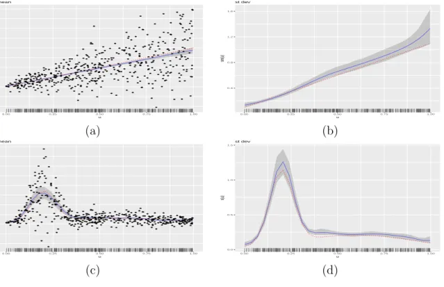
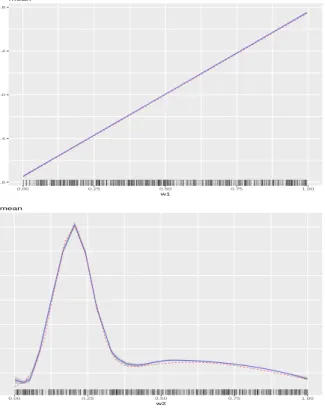
The resulting plots can be seen in Figure 2, panels (a) and (b). Panel (a) displays the simulated dataset, showing the expected increase in both the mean and variance with increasing values of the covariate u. Further, we see the posterior mean of µ(u) = β0 +fµ(u) = β0 +P21j=1βjφ1j(u) evaluated over a grid
of 30 values of u, as specified by the (default) grid = 30 option in function plot. For each sample
β(s), s = 1, . . . , S,from the posterior ofβ, and for each value ofuover the grid of 30 values,uj, j = 1, . . . ,30,
functionplotcomputesµ(uj)(s) =β0(s)+
P21
j=1β
(s)
j φ1j(uj). The default optionintercept = TRUEspecifies
that the interceptβ0 is included in the computation, but it may be removed by settingintercept = FALSE.
The posterior means are computed by the usual ¯µ(uj) =S−1
P
sµ(uj)(s) and are plotted with solid
(blue-color) line. By default, the function displays 80% point-wise credible intervals (CI). In Figure 2 panel (a) we have plotted 99% CIs, as specified by option quantiles = c(0.005, 0.995). This option specifies that for each value uj, j = 1, . . . ,30,on the grid, 99% CIs for µ(uj) are computed by the 0.5% and 99.5%
● ●●● ● ● ● ●● ● ● ●● ● ● ● ● ● ● ● ● ● ● ● ● ● ● ● ● ● ● ● ● ● ● ●● ● ● ● ● ● ● ● ● ● ● ● ●● ● ● ● ● ● ● ● ● ● ● ● ● ●● ● ● ● ● ● ● ● ● ● ● ● ● ● ● ● ● ● ● ● ● ● ● ● ● ● ● ● ● ● ● ● ● ● ● ● ● ● ● ● ● ● ● ● ● ● ● ● ● ●● ● ● ● ● ● ● ● ● ● ● ● ●● ● ● ● ● ● ● ● ● ● ● ● ● ● ● ● ● ● ● ● ● ● ● ● ● ● ● ●●●●● ● ● ● ● ● ● ● ● ● ● ● ● ● ● ● ● ● ● ● ● ●● ● ● ● ● ● ● ● ● ● ● ● ● ● ● ● ● ● ● ● ● ● ● ● ● ● ● ● ● ● ● ● ● ● ● ● ● ● ● ● ● ● ● ● ● ● ● ● ● ● ● ● ● ● ● ● ● ● ● ● ● ● ● ● ● ● ● ● ● ● ● ● ● ● ● ● ● ● ● ● ● ● ● ● ● ● ● ● ● ● ● ● ● ● ● ● ● ● ● ● ● ● ● ● ● ● ● ● ● ● ● ● ● ● ● ● ● ● ● ● ● ● ● ● ● ● ● ● ● ●● ● ● ● ● ● ● ●● ● ● ● ● ● ● ● ● ● ● ● ● ● ● ● ● ● ● ● ● ● ● ● ● ● ● ● ● ● ● ● ● ● ● ●● ● ● ● ● ● ● ● ● ● ● ● ● ● ● ● ● ● ● ●● ● ● ● ● ● ● ● ● ● ● ● ● ● ● ● ● ● ● ● ● ● ● ● ● ●● ● ● ● ● ● ● ● ● ● ● ● ● ● ● ● ● ● ● ● ● ● ● ● ● ● ● ● ● ● ● ● ● ● ● ● ● ● ● ● ● ● ● ● ● ● ● ● ● ● ● ● ● ● ● ● ● ● ● ● ● ● ● ● ● ● ● ● ● ● ● ● ● ● ● ● ● ● ● ● ● ● ● ● ● ● ● ● ● ● ● ● ● ● ● ● ● ● ● ●● −1 0 1 2 3 4 0.00 0.25 0.50 0.75 1.00 u sm(u) mean 0.4 0.8 1.2 1.6 0.00 0.25 0.50 0.75 1.00 u sm(u) st dev (a) (b) ● ●●● ●● ● ●●● ● ●● ● ● ● ● ● ● ● ● ● ● ● ● ● ● ● ● ● ● ● ● ● ● ● ● ● ● ● ● ● ● ● ● ● ● ● ● ● ● ● ● ● ● ● ● ● ● ● ● ● ● ● ● ● ● ● ● ● ● ● ● ● ● ● ● ● ● ● ● ● ● ● ● ● ● ● ● ● ● ● ● ● ● ● ● ● ● ● ● ● ● ● ● ● ● ● ● ● ● ● ● ● ● ● ● ● ● ● ● ● ● ● ● ●● ● ● ● ● ● ● ● ● ● ● ● ● ● ● ● ● ● ● ● ● ● ● ● ● ● ● ●●●●● ● ● ● ● ● ● ● ● ● ● ● ● ● ● ● ● ● ● ● ● ●● ● ● ● ● ● ● ● ● ● ● ● ● ● ● ● ● ● ● ● ● ● ●● ● ● ● ● ● ● ● ● ● ● ● ● ● ● ● ● ● ● ● ● ● ● ● ● ● ● ● ● ● ●● ● ● ● ● ● ● ● ● ● ● ● ● ● ● ● ● ● ● ● ● ● ● ● ● ● ● ● ● ● ● ● ● ● ● ● ● ● ● ● ●● ● ● ● ● ● ● ● ● ● ● ● ● ● ● ●● ●● ● ● ● ● ● ● ●● ● ● ● ● ● ● ● ●● ● ● ● ● ● ● ●● ● ● ● ● ● ● ●● ● ● ● ● ● ● ●● ●● ● ●● ● ●● ● ● ● ● ●● ● ● ● ● ●● ● ● ● ● ● ● ●● ● ● ● ● ● ● ● ● ● ● ●● ● ● ● ● ● ● ● ● ● ● ● ● ●● ● ● ● ● ● ● ● ● ● ● ●●● ● ● ● ● ● ● ● ● ● ● ● ●● ● ● ● ● ● ● ● ● ● ● ● ● ● ● ● ● ● ● ●● ● ● ● ● ● ● ● ● ● ● ● ● ● ●● ●● ● ●● ● ● ● ● ● ●●● ● ● ● ● ● ● ● ● ● ● ● ● ● ● ● ● ● ●● ● ● ● ● ● ● ● ● ● ● ● ● ● ● ● ● ● ●● −1 0 1 2 3 4 0.00 0.25 0.50 0.75 1.00 u s(u) mean 0.0 0.5 1.0 1.5 0.00 0.25 0.50 0.75 1.00 u s(u) st dev (c) (d)
Figure 2: Results from the single covariate simulated examples. The column on the left-hand side displays the generated data points and posterior means of the estimated effect along with 99% CIs. The column on the right-hand side displays the posterior mean of the estimated standard deviation function along with 90% CIs. In all panels, the truth is represented by dashed (red color) lines, the posterior means by solid (blue color) lines, and the CIs by gray color.
quantiles of the samplesµ(uj)(s), s= 1, . . . , S. Plots without credible intervals may be obtained by setting
quantiles = NULL.
Figure 2, panel (b) displays the posterior mean of the standard deviation function, given by σ(u) = σexp{Pq2
j=1αjφ2j(u)/2}. The details are the same as for the plot of the mean function, so here we briefly
mention a difference: option intercept = TRUEspecifies that σ is included in the calculation. It may be removed by setting intercept = FALSE, which will result in plots of σ(u)∗ = exp{Pq2
j=1αjφ2j(u)/2}.
We use the second simulated dataset to show how thes constructor from package mgcvmay be used. In our example, we used s to specify the model as follows
> model <- y ~ s(u, k = 15, bs = "ps", absorb.cons=TRUE) |
+ s(u, k = 15, bs = "ps", absorb.cons=TRUE)
Function BNSP::scalls in turn mgcv::sand mgcv::smoothCon. All options of the last two functions may be passed to BNSP::s. In the example above we used options k, bs and absorb.cons.
The remaining R code for the second simulated example is precisely the same as the one for the first example, and hence omitted. Results are shown in Figure 2, panels (c) and (d).
We conclude the current section by describing the function predict.mvrm. The function provides predictions and posterior credible or prediction intervals for given feature vectors. The two types of intervals differ in the associated level of uncertainty: prediction intervals attempt to capture a future response and are usually much wider than credible intervals that attempt to capture a mean response.
The following code shows how credible and prediction intervals can be obtained for a sequence of covariate values stored in x1
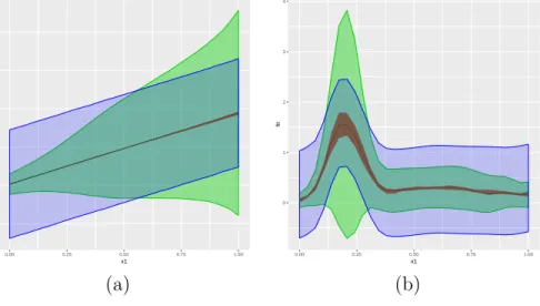
0 2 4 0.00 0.25 0.50 0.75 1.00 x1 fit 0 1 2 3 4 0.00 0.25 0.50 0.75 1.00 x1 fit (a) (b)
Figure 3: Predictions results from the first two simulated datasets. Each panel displays a credible interval and two prediction intervals, one obtained using a model that recognizes the dependence of the variance on the covariate and one that ignores it.
> x1 <- seq(0, 1, length.out = 30)
> p1 <- predict(m1, newdata = data.frame(u = x1), interval = "credible") > p2 <- predict(m1, newdata = data.frame(u = x1), interval = "prediction")
where the first argument in function predict is a fitted mvrm model, the second one is a data frame containing the feature vectors at which predictions are to be obtained and the last one defines the type of interval to be created. We applied the predict function to the two simulated datasets. To each of those datasets we fitted two models: the first one is the one we saw earlier, where both the mean and variance are modeled in terms of covariates, while the second one ignores the dependence of the variance on the covariate. The latter model is specified in R using
> model <- y ~ sm(u, k = 20, bs = "rd") | 1
Results are displayed in Figure 3. Each of the two figures displays a credible interval and two prediction intervals. The figure emphasizes a point that was discussed in the introductory section, that modeling the variance in terms of covariates can result in more realistic prediction intervals. The same point was recently discussed by Mayr et al. (2012).
3.1.2 Bivariate covariate case
Interactions between two predictors can be modeled by appropriate specification of either the built-in sm
function or the smooth constructors frommgcv. Functionsm can take up to two covariates, both of which may be continuous or one continuous and one discrete. Next we consider an example that involves two continuous covariates. An example involving a continuous and a discrete covariate is shown later on, in the second application to a real dataset.
Letu= (u1, u2)> denote a bivariate predictor. The data-generating mechanism that we consider is y(u)∼N{µ(u), σ2(u)}, µ(u) = 0.1 +N(u,µ1,Σ1) +N(u,µ2,Σ2), σ2(u) = 0.1 +{N(u,µ1,Σ1) +N(u,µ2,Σ2)}/2, µ1 = 0.25 0.75 ,Σ1 = 0.03 0.01 0.01 0.03 ,µ2 = 0.65 0.35 ,Σ2 = 0.09 0.01 0.01 0.09 .
As before, u1 and u2 are obtained independently from uniform distributions on the unit interval. Further,
the sample size is set to n = 500.
In R, we simulate data from the above mechanism using
> mu1 <- matrix(c(0.25, 0.75))
> sigma1 <- matrix(c(0.03, 0.01, 0.01, 0.03), 2, 2) > mu2 <- matrix(c(0.65, 0.35))
> sigma2 <- matrix(c(0.09, 0.01, 0.01, 0.09), 2, 2) > mu <- function(x1, x2) {x <- cbind(x1, x2);
+ 0.1 + dmvnorm(x, mu1, sigma1) + dmvnorm(x, mu2, sigma2)}
> Sigma <- function(x1, x2) {x <- cbind(x1, x2);
+ 0.1 + (dmvnorm(x, mu1, sigma1) + dmvnorm(x, mu2, sigma2)) / 2}
> set.seed(1) > n <- 500
> w1 <- runif(n) > w2 <- runif(n) > y <- vector()
> for (i in 1 : n) y[i] <- rnorm(1, mean = mu(w1[i], w2[i]),
+ sd = sqrt(Sigma(w1[i], w2[i])))
> data <- data.frame(y, w1, w2)
We fit a model with mean and variance functions specified as
µ(u) =β0+ 12 X j1=1 12 X j2=1 βj1,j2φ1j1,j2(u), log(σ 2 (u)) =α0+ 12 X j1=1 12 X j2=1 αj1,j2φ2j1,j2(u).
The R code that fits the above model is
> Model <- y ~ sm(w1, w2, k = 10, bs = "rd") | sm(w1, w2, k = 10, bs = "rd") > m2 <- mvrm(formula = Model, data = data, sweeps = 10000, burn = 5000, thin = 2,
+ seed = 1, StorageDir = DIR)
As in the univariate case, convergence assessment and univariate posterior summaries may be obtained by using function mvrm2mcmc in conjunction with functions plot.mcmc and summary.mcmc. Further, sum-maries of the ‘mvrm’ fits may be obtained using functions print.mvrm and summary.mvrm. Plots of the bivariate effects may be obtained using function plot.mvrm. This is shown below, where argument
plotOptions utilizes package colorspace (Zeileis et al., 2009).
> plot(x = m2, model = "mean", term = "sm(w1,w2)", static = TRUE,
+ plotOptions = list(col = diverge_hcl(n = 10)))
> plot(x = m2, model = "stdev", term = "sm(w1,w2)", static = TRUE,
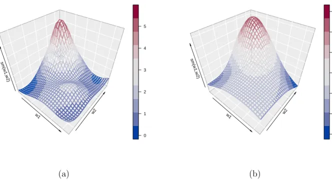
w1 w2 sm(w1,w2) mean 0 1 2 3 4 5 w1 w2 sm(w1,w2) st dev 0.4 0.6 0.8 1.0 1.2 1.4 1.6 (a) (b)
Figure 4: Bivariate simulation study results with two continuous covariates. Posterior means of the (a) mean and (b) standard deviation function.
Results are shown in Figure 4. For bivariate predictors, function plot.mvrm calls function ribbon3D
from package plot3D. Dynamic plots, viewable in a browser, can be created by replacing the default
static = TRUE by static = FALSE. When the latter option is specified, function plot.mvrm calls func-tion scatterplot3js from package threejs. Users may pass their own options to plot.mvrm via the
plotOptions argument.
3.1.3 Multiple covariate case
We consider fitting general additive models for the mean and variance functions in a simulated example with four independent continuous covariates. In this scenario, we set n = 1000. Further the covariates
w = (w1, w2, w3, w4)> are simulated independently from a uniform distribution on the unit interval. The
data-generating mechanism that we consider is
Y(w)∼N(µ(w), σ2(w)), µ(w) = 4 X j=1 µj(wj) and σ(w) = 4 Y j=1 σj(wj)
where functions µj, σj, j = 1, . . . ,4, are specified below
1. µ1(w1) = 1.5w1, σ1(w1) = {N(w1, µ = 0.2, σ2 = 0.004) +N(w1, µ= 0.6, σ2 = 0.1)}/2,
2. µ2(w2) ={N(w2, µ = 0.2, σ2 = 0.004) +N(w2, µ= 0.6, σ2 = 0.1)}/2,
σ2(w2) = 0.6 + 0.5 sin(2πw2),
4. µ4(w4) =−w4, σ4(w4) = 0.2 + 1.5w4.
To the generated dataset we fit a model with mean and variance functions modeled as
µ(w) =β0+ 4 X k=1 16 X j=1 βkjφkj(wk) and log{σ2(w)}=α0+ 4 X k=1 16 X j=1 αkjφkj(wk).
Fitting the above model to the simulated data is achieved by the following R code
> Model <- y ~ sm(w1, k = 15, bs = "rd") + sm(w2, k = 15, bs = "rd") + + sm(w3, k = 15, bs = "rd") + sm(w4, k = 15, bs = "rd") | + sm(w1, k = 15, bs = "rd") + sm(w2, k = 15, bs = "rd") + + sm(w3, k = 15, bs = "rd") + sm(w4, k = 15, bs = "rd") > m3 <- mvrm(formula = Model, data = data, sweeps = 50000, burn = 25000,
+ thin = 5, seed = 1, StorageDir = DIR)
By default function sm utilizes the radial basis functions, hence there is no need to specify bs = "rd" as we did earlier, if radial basis functions are preferred over thin plate splines. Further, we have selected k = 15 for all smooth functions. However, there is no restriction to the number of knots and certainly one can select a different number of knots for each smooth function.
As discussed previously, for each term that appears in the right-hand side of the mean and variance functions, the model incorporates indicator variables that specify which basis functions are to be included and which are to be excluded from the model. For the current example, the indicator variables are denoted byγkj andδkj, k= 1,2,3,4, j = 1, . . . ,16. The prior probabilities that variables are included were specified
in (8) and they are specific to each term, πµk ∼ Beta(cµk, dµk), πσk ∼ Beta(cσk, dσk), k = 1,2,3,4.
The default option pi.muPrior = "Beta(1,1)" specifies that πµk ∼ Beta(1,1), k = 1,2,3,4. Further,
by setting, for example, pi.muPrior = "Beta(2,1)" we specify that πµk ∼ Beta(2,1), k = 1,2,3,4. To
specify a different Beta prior for each of the four terms, pi.muPrior will have to be specified as a vector of length four, as an example, pi.muPrior = c("Beta(1,1)","Beta(2,1)","Beta(3,1)","Beta(4,1)"). Specification of the priors for πσk is done in a similar way, via argument pi.sigmaPrior.
We conclude this section by presenting plots of the four terms in the mean and variance models. The plots are presented in Figure 5. We provide a few details on how function plot works in the presence of multiple terms, and how the comparison between true and estimated effects is made. Starting with the mean function, to create the relevant plots, that appear on the left panels of Figure 5, function plot
considers only the part of the mean functionµ(u) that is related to the chosentermwhile leaving all other terms out. For instance, in the code below we choose term = "sm(u1)" and hence we plot the posterior mean and a posterior credible interval for P16
j=1β1jφ1j(u1), where the intercept β0 is left out by option
intercept = FALSE. Further, comparison is made with a centered version of the true curve, represented by the dashed (red color) line and obtained by the first three lines of code below.
> x1 <- seq(0, 1, length.out = 30) > y1 <- mu1(x1)
> y1 <- y1 - mean(y1)
> PlotOptions <- list(geom_line(aes_string(x = x1, y = y1),
+ col = 2, alpha = 0.5, lty = 2))
> plot(x = m3, model = "mean", term = "sm(w1)", plotOptions = PlotOptions,
The plots of the four standard deviation terms are shown in the right panels of Figure 5. Again, these are created by considering only the part of the model forσ(u) that is related to the chosenterm. For instance, below we chooseterm = "sm(u1)". Hence, in this case the plot will present the posterior mean and a pos-terior credible interval for exp{P16
j=1α1jφ1j(u1)/2}, where the interceptα0 is left out by optionintercept
= FALSE. Option centreEffects = TRUE scales the posterior realizations of exp{P16
j=1α1jφ1j(u1)/2}
be-fore plotting them, where the scaling is done in such a way that the realized function has mean one over the range of the predictor. Further, the comparison is made with a scaled version of the true curve, where again the scaling is done to achieve mean one. This is shown below and it is in the spirit of Chan et al. (2006) who discuss the differences between the data generating mechanism and the fitted model.
> y1 <- stdev1(x1) / mean(stdev1(x1))
> PlotOptions <- list(geom_line(aes_string(x = x1, y = y1),
+ col = 2, alpha = 0.5, lty = 2))
> plot(x = m3, model = "stdev", term = "sm(w1)", plotOptions = PlotOptions,
+ intercept = FALSE, centreEffects = TRUE, quantiles = c(0.025, 1 - 0.025))
3.2
Data analyses
In this section we present four empirical applications. 3.2.1 Wage and age
In the first empirical application, we analyse a dataset from Pagan & Ullah (1999) that is available in the R packagenp(Hayfield & Racine, 2008). The dataset consists ofn= 205 observations on dependent variable
logwage, the logarithm of the individual’s wage, and covariateage, the individual’s age. The dataset comes from the 1971 Census of Canada Public Use Sample Tapes and the sampling units it involves are males of common education. Hence, the investigation of the relationship between age and the logarithm of wage is carried out controlling for the two potentially important covariates education and gender.
We utilize the following R code to specify flexible models for the mean and variance functions, and to obtain 5,000 posterior samples, after a burn-in period of 25,000 samples and a thinning period of 5.
> data(cps71) > DIR <- getwd()
> model <- logwage ~ sm(age, k = 30, bs = "rd") | sm(age, k = 30, bs = "rd") > m4 <- mvrm(formula = model, data = cps71, sweeps = 50000,
+ burn = 25000, thin = 5, seed = 1, StorageDir = DIR)
After checking convergence, we use the following code to create the plots that appear in Figure 6.
> wagePlotOptions <- list(geom_point(data = cps71, aes(x = age, y = logwage))) > plot(x = m4, model = "mean", term = "sm(age)", plotOptions = wagePlotOptions) > plot(x = m4, model = "stdev", term = "sm(age)")
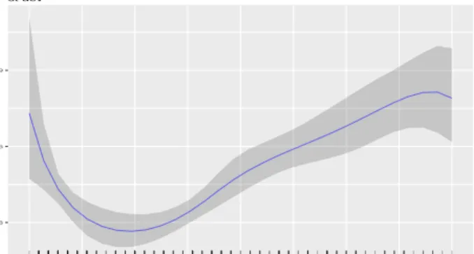
Figure 6 (a) shows the posterior mean and an 80% credible interval for the mean function and it suggests a quadratic relationship between age and logwage. Figure 6 (b) shows the posterior mean and an 80% credible interval for the standard deviation function. It suggest a complex relationship between age and the variability in logwage. The relationship suggested by Figure 6 (b) is also suggested by the spread of the data-points around the estimated mean in Figure 6 (a). At ages around 20 years the variability in
−0.8 −0.4 0.0 0.4 0.8 0.00 0.25 0.50 0.75 1.00 w1 sm(w1) mean 0 1 2 3 4 0.00 0.25 0.50 0.75 1.00 w1 sm(w1) st dev 0 1 2 0.00 0.25 0.50 0.75 1.00 w2 sm(w2) mean 0.5 1.0 1.5 2.0 0.00 0.25 0.50 0.75 1.00 w2 sm(w2) st dev −1.0 −0.5 0.0 0.5 1.0 0.00 0.25 0.50 0.75 1.00 w3 sm(w3) mean 0.5 1.0 1.5 2.0 0.00 0.25 0.50 0.75 1.00 w3 sm(w3) st dev −0.50 −0.25 0.00 0.25 0.50 0.00 0.25 0.50 0.75 1.00 w4 sm(w4) mean 0.5 1.0 1.5 2.0 0.00 0.25 0.50 0.75 1.00 w4 sm(w4) st dev
Figure 5: Multiple covariate simulation study results. The column on the left-hand side presents the true and estimated mean functions, along with 99% credible intervals. The column on the right-hand side presents the true and estimated standard deviation functions, along with 95% credible intervals. In all panels, the truth is represented by dashed (red color) lines, the estimated functions by solid (blue color) lines, and the credible intervals by gray color.
● ● ● ● ● ● ● ● ● ● ● ● ● ● ● ● ● ● ● ● ● ● ● ● ● ● ● ● ● ● ● ● ● ● ● ● ● ● ● ● ● ● ● ● ● ● ● ● ● ● ● ● ● ● ● ● ● ● ● ● ● ● ● ● ● ● ● ● ● ● ● ● ● ● ● ● ●● ● ● ● ● ● ● ● ● ● ● ● ● ● ● ● ● ● ● ● ● ●● ● ● ● ● ● ● ● ● ● ● ● ● ● ● ● ● ● ● ● ● ● ● ● ● ● ● ● ● ● ● ● ● ● ● ● ● ● ● ● ● ● ● ● ● ● ● ● ● ● ● ● ● ● ● ●● ● ● ● ● ● ● ● ● ● ● ● ● ● ● ● ● ● ● ● ● ● ● ● ● ● ● ● ● ● ● ● ● ● ● ● ● ● ● ● ● ● ● ● ● ● ● ● ● ● 11 12 13 14 15 0.00 0.25 0.50 0.75 1.00 nage sm(nage) mean 0.3 0.6 0.9 0.00 0.25 0.50 0.75 1.00 nage sm(nage) st dev (a) (b)
Figure 6: Results from the data analysis on the relationship between age and the logarithm of wage. Panel (a) shows the posterior mean and an 80% credible interval of the mean function, and the observed data-points. Panel (b) shows the posterior mean and an 80% credible interval of the standard deviation function.
logwage is high. It then reduces until about age 30, to start increasing again until about age 45. From age 45 to 60 it remains stable but high, while for ages above 60, Figure 6 (b) suggests further increase in the variability, but the wide credible interval suggests high uncertainty over this age range.
3.2.2 Wage and multiple covariates
In the second empirical application, we analyse a dataset from Wooldridge (2008) that is also available in R package np. The response variable here is the logarithm of the individual’s hourly wage (lwage) while the covariates include the years of education (educ), the years of experience (exper), the years with the current employer (tenure), the individual’s gender (named as female within the dataset, with levels
Female and Male), and marital status (named as married with levels Married and Notmarried). The dataset consists of n = 526 independent observations. We analyse the first three covariates as continuous and the last two as discrete.
As the variance function is modeled in terms of an exponential, see (1), to avoid potential numerical problems, we transform the three continuous variables to have range in the interval [0,1], using
> data(wage1)
> wage1$ntenure <- wage1$tenure / max(wage1$tenure) > wage1$nexper <- wage1$exper / max(wage1$exper) > wage1$neduc <- wage1$educ / max(wage1$educ)
We choose to fit the following mean and variance models to the data
µi =β0+β1 marriedi+f1(ntenurei) +f2(neduci) +f3(nexperi,femalei),
log(σ2i) =α0+f4(nexperi).
We note that, as it turns out, an interaction between variablesnexper and femaleis not necessary for the current data analysis. However, we choose to add this term in the mean model in order to illustrate how interaction terms can be specified. We illustrate further options below.
> knots2 <- c(0, 1)
> knotsD <- expand.grid(knots1, knots2)
> model <- lwage ~ fmarried + sm(ntenure) + sm(neduc, knots=data.frame(knots = + seq(min(wage1$neduc), max(wage1$neduc), length.out = 15))) +
+ sm(nexper, ffemale, knots = knotsD) | sm(nexper, knots=data.frame(knots = + seq(min(wage1$nexper), max(wage1$nexper), length.out=15)))
The first three lines of the R code above specify the matrix of (potential) knots to be used for representing f3(nexper,female). Knots may be left unspecified, in which case the defaults in functionsm will be used.
Furthermore, in the specification of the mean model we use sm(ntenure). By this, we chose to represent f1 utilizing the default 10 knots and the radial basis functions. Further, the specification off2 in the mean
model illustrates how users can specify their own knots for univariate functions. In the current example, we select 15 knots uniformly spread over the range of neduc. Fifteen knots are also used to represent f4
within the variance model.
The following code is used to obtain samples from the posteriors of the model parameters.
> DIR <- getwd()
> m5 <- mvrm(formula = model, data = wage1, sweeps = 100000,
+ burn = 25000, thin = 5, seed = 1, StorageDir = DIR))
After summarizing results and checking convergence, we create plots of posterior means, along with 95% credible intervals, for functions f1, . . . , f4. These are displayed in Figure 7. As it turns out, variable
married does not have an effect on the mean of lwage. For this reason, we do not provide further results on the posterior of the coefficient of covariate married, β1. However, in the code below we show how
graphical summaries on β1 can be obtained, if needed.
> PlotOptionsT <- list(geom_point(data = wage1, aes(x = ntenure, y = lwage))) > plot(x = m5, model = "mean", term="sm(ntenure)", quantiles = c(0.025, 0.975),
+ plotOptions = PlotOptionsT)
> PlotOptionsEdu <- list(geom_point(data = wage1, aes(x = neduc, y = lwage))) > plot(x = m5, model = "mean", term = "sm(neduc)", quantiles = c(0.025, 0.975),
+ plotOptions = PlotOptionsEdu)
> pchs <- as.numeric(wage1$female)
> pchs[pchs == 1] <- 17; pchs[pchs == 2] <- 19 > cols <- as.numeric(wage1$female)
> cols[cols == 2] <- 3; cols[cols == 1] <- 2
> PlotOptionsE <- list(geom_point(data = wage1, aes(x = nexper, y = lwage),
+ col = cols, pch = pchs, group = wage1$female))
> plot(x = m5, model = "mean", term="sm(nexper,female)", quantiles = c(0.025, 0.975),
+ plotOptions = PlotOptionsE)
> plot(x = m5, model = "stdev", term = "sm(nexper)", quantiles = c(0.025, 0.975)) > PlotOptionsF <- list(geom_boxplot(fill = 2, color = 1))
> plot(x = m5, model = "mean", term = "married", quantiles = c(0.025, 0.975),
+ plotOptions = PlotOptionsF)
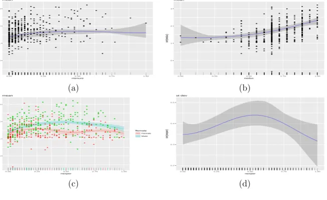
Figure 7, panels (a) and (b) show the posterior means and 95% credible intervals forf1(ntenure) and
f2(neduc). It can be seen that expected wages increase with tenure and education, although there is high
uncertainty over a large part of the range of both covariates. Panel (c) displays the posterior mean and a 95% credible interval for f3. We can see that although the forms of the two functions are similar, i.e. the
● ● ● ● ● ● ● ● ● ● ● ● ● ● ● ● ● ● ● ● ● ● ● ● ● ● ● ● ● ● ● ● ● ● ● ● ● ● ● ● ● ● ● ● ● ● ● ● ● ● ● ● ● ● ● ●● ● ● ● ● ● ● ● ● ● ● ● ● ● ● ● ● ● ● ● ● ● ● ● ● ● ● ● ● ● ● ● ● ● ● ● ● ● ● ● ● ● ● ● ● ● ● ● ● ● ● ● ● ● ● ● ● ● ● ● ●●● ● ● ● ● ● ● ● ● ● ● ● ● ● ● ● ● ● ● ● ● ● ● ● ● ● ● ● ● ● ● ● ● ● ● ● ● ● ● ● ● ● ● ● ● ● ● ● ● ● ● ● ● ● ● ● ● ● ● ● ● ● ● ● ● ● ● ● ● ● ● ● ● ● ● ● ● ● ● ● ● ● ● ● ● ● ● ● ● ● ● ● ● ● ● ● ● ● ● ● ● ● ● ● ● ● ● ● ● ● ● ● ● ● ● ● ● ● ● ● ● ● ● ● ● ● ● ● ● ● ● ● ● ● ● ● ● ● ● ● ● ● ● ● ● ● ● ● ● ● ● ● ● ● ● ● ● ● ● ● ● ● ● ● ● ● ● ● ● ● ● ● ● ● ● ● ● ● ● ● ● ● ● ● ● ● ● ● ● ● ● ● ● ● ● ● ● ● ● ● ● ● ● ● ● ● ● ● ● ● ● ● ● ● ● ● ● ● ● ● ● ● ● ● ● ● ● ● ● ● ● ● ● ● ● ● ● ● ● ● ● ● ● ● ● ● ● ● ● ● ● ● ● ● ● ● ● ● ● ● ● ● ● ● ● ● ● ● ● ● ● ● ● ● ● ● ● ● ● ● ● ● ● ● ● ● ● ● ● ● ● ● ● ● ● ● ● ● ● ● ● ● ● ● ● ● ● ● ● ● ● ● ● ● ● ● ● ● ● ● ● ● ● ● ● ● ● ● ● ● ● ● ● ● ● ● ● ● ● ● ● ● ● ● ● ● ● ● ● ● ● ● ● ● ● ● ● ● ● ● ● ● ● ● ● ● ● ● ● ● ● ● ● ● ● ● ● ● ● ● ● ● ● ● ● ● ● ● ● ● ● ● ● ● ● ● ● ● ● ● ● ● ● ● ● ● ● ● 0 1 2 3 0.00 0.25 0.50 0.75 1.00 ntenure sm(nten ure) mean ● ● ● ● ● ● ● ● ● ● ● ● ● ● ● ● ● ● ● ● ● ● ● ● ● ● ● ● ● ● ● ● ● ● ● ● ● ● ● ● ● ● ● ● ● ● ● ● ● ● ● ● ● ● ● ● ● ● ● ● ● ● ● ● ● ● ● ● ● ● ● ● ● ● ● ● ● ● ● ● ● ● ● ● ● ● ● ● ● ● ● ● ● ● ● ● ● ● ● ● ● ● ● ● ● ● ● ● ● ● ● ● ● ● ● ● ● ● ● ● ● ● ● ● ● ● ● ● ● ● ● ● ● ● ● ● ● ● ● ● ● ● ● ● ● ● ● ● ● ● ● ● ● ● ● ● ● ● ● ● ● ● ● ● ● ● ● ● ● ● ● ● ● ● ● ● ● ● ● ● ● ● ● ● ● ● ● ● ● ● ● ● ● ● ● ● ● ● ● ● ● ● ● ● ● ● ● ● ● ● ● ● ● ● ● ● ● ● ● ● ● ● ● ● ● ● ● ● ● ● ● ● ● ● ● ● ● ● ● ● ● ● ● ● ● ● ● ● ● ● ● ● ● ● ● ● ● ● ● ● ● ● ● ● ● ● ● ● ● ● ● ● ● ● ● ● ● ● ● ● ● ● ● ● ● ● ● ● ● ● ● ● ● ● ● ● ● ● ● ● ● ● ● ● ● ● ● ● ● ● ● ● ● ● ● ● ● ● ● ● ● ● ● ● ● ● ● ● ● ● ● ● ● ● ● ● ● ● ● ● ● ● ● ● ● ● ● ● ● ● ● ● ● ● ● ● ● ● ● ● ● ● ● ● ● ● ● ● ● ● ● ● ● ● ● ● ● ● ● ● ● ● ● ● ● ● ● ● ● ● ● ● ● ● ● ● ● ● ● ● ● ● ● ● ● ● ● ● ● ● ● ● ● ● ● ● ● ● ● ● ● ● ● ● ● ● ● ● ● ● ● ● ● ● ● ● ● ● ● ● ● ● ● ● ● ● ● ● ● ● ● ● ● ● ● ● ● ● ● ● ● ● ● ● ● ● ● ● ● ● ● ● ● ● ● ● ● ● ● ● ● ● ● ● ● ● ● ● ● ● ● ● ● ● ● ● ● ● ● ● ● ● ● ● ● ● ● ● ● ● ● ● ● ● ● ● ● ● ● ● ● ● ● ● ● ● 0 1 2 3 0.00 0.25 0.50 0.75 1.00 neduc sm(neduc) mean (a) (b) ● ● ● ● ● ● ● ● ● ● ● ● ● ● ● ● ● ● ● ● ● ● ● ● ● ● ● ● ● ● ● ● ● ● ● ● ● ● ● ● ● ● ● ● ● ● ● ● ● ● ● ● ● ● ● ● ● ● ● ● ● ● ● ● ● ● ● ● ● ● ● ● ● ● ● ● ● ● ● ● ● ● ● ● ● ● ● ● ● ● ● ● ● ● ● ● ● ● ● ● ● ● ● ● ● ● ● ● ● ● ● ● ● ● ● ● ● ● ● ● ● ● ● ● ● ● ● ● ● ● ● ● ●● ● ● ● ● ● ● ● ● ● ● ● ● ● ● ● ● ● ● ● ●● ● ● ● ● ● ● ● ● ● ● ● ● ● ● ● ● ● ● ● ● ● ● ● ● ● ● ● ● ● ● ● ● ● ● ● ● ● ● ● ● ● ● ● ● ● ● ● ● ● ● ● ● ● ● ● ● ● ● ● ● ● ● ● ● ● ● ● ● ● ● ● ● ● ● ● ● ● ● ● ● ● ● ● ● ● ● ● ● ● ● ● ● ● ● ● ● ● ● ● ● ● ● ● ● ● ● ● ● ● ● ● ● ● ● ● ● ● ● ● 0 1 2 3 0.00 0.25 0.50 0.75 1.00 nexper sm(ne xper ,ffemale) ffemale Female Male mean 0.2 0.3 0.4 0.5 0.00 0.25 0.50 0.75 1.00 nexper sm(ne xper) st dev (c) (d)
Figure 7: Results from the data analysis on the relationship between covariates gender, marital status, experience, education and tenure, and response variable logarithm of hourly wage. Posterior means and 95% credible intervals for (a) f1(ntenure), (b) f2(neduc), (c) f3(nexper,female), and (d) the standard
deviation function σi =σexp[f4(nexper)/2].
interaction term is not needed, males have higher expected wages than females. Lastly, panel (d) displays posterior summaries of the standard deviation function, σi =σexp(f4/2). It can be seen that variability
first increases and then decreases as experience increases.
Lastly, we obtain predictions and credible intervals for the levels "Married" and "Notmarried" of variable fmaried and the levels"Female" and "Male" of variable ffemale, with variables ntenure, nedc
and nexper fixed at their mid-range.
> p1 <- predict(m5, newdata = data.frame(fmarried = rep(c("Married", "Notmarried"), 2),
+ ntenure = rep(0.5, 4), neduc = rep(0.5, 4), nexper = rep(0.5, 4),
+ ffemale = rep(c("Female", "Male"), each = 2)), interval = "credible") > p1 fit lwr upr 1 1.321802 1.119508 1.506574 2 1.320400 1.119000 1.505272 3 1.913341 1.794035 2.036255 4 1.911939 1.791578 2.034832
The predictions are suggestive of no ‘marriage’ effect and of ‘gender’ effect. 3.2.3 Brain activity
Here we analyse brain activity level data obtained by functional magnetic resonance imaging. The dataset is available in package gamair (Wood, 2006) and it was previously analysed by Landau et al. (2003). We
are interested in three of the columns in the dataset. These are the response variable, medFPQ, which is calculated as the median over three measurements of ‘Fundamental Power Quotient’ and the two covariates,
X and Y, which show the location of each voxel.
The following R code loads the relevant data frame, removes two outliers and transforms the response variable, as was suggested by Wood (2006). In addition, it plots the brain activity data using function
levelplot from package lattice (Sarkar, 2008).
> data(brain)
> brain <- brain[brain$medFPQ > 5e-5, ] > brain$medFPQ <- (brain$medFPQ) ^ 0.25
> levelplot(medFPQ ~ Y * X, data = brain, xlab = "Y", ylab = "X",
+ col.regions = gray(10 : 100 / 100))
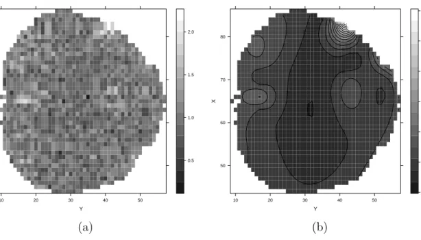
The plot of the observed data is shown in Figure 8, panel (a). Its distinctive feature is the noise level, which makes difficult to decipher any latent pattern. Hence, the goal of the current data analysis is to obtain a smooth surface of brain activity level from the noisy data. It was argued by Wood (2006) that for achieving this goal a spatial error term is not needed in the model. Thus, we analyse the brain activity level data using a model of the form
medFPQi ind∼ N(µi, σ2), whereµi =β0+ 10 X j1=1 10 X j2=1 βj1,j2φ1j1,j2(Xi, Yi), i= 1, . . . , n,
where n = 1565 is the number of voxels. The R code that fits the above model is
> Model <- medFPQ ~ sm(Y, X, k = 10, bs = "rd") | 1
> m6 <- mvrm(formula = Model, data = brain, sweeps = 50000, burn = 20000, thin = 2,
+ seed = 1, StorageDir = DIR)
From the fitted model we obtain a smooth brain activity level surface using function predict. The function estimates the average activity at each voxel of the brain. Further, we plot the estimated surface using function levelplot.
> p1 <- predict(m6)
> levelplot(p1[, 1] ~ Y * X, data = brain , xlab = "Y", ylab = "X",
+ col.regions = gray(10 : 100 / 100), contour = TRUE)
Results are shown in Figure 8, panel(b). The smooth surface makes it much easier to see and understand which parts of the brain have higher activity.
3.2.4 Cars
In the fourth and final application we use function mvrm to identify the best subset of predictors in a regression setting. Usually stepwise model selection is performed, using functionsstep and stepAICin R. Here we show how mvrm can be used as alternative to those two functions. The data frame that we apply
mvrm on is mtcars, where the response variable is mpg and the explanatory variables that we consider are
disp, hp, wt and qsec. The code below loads the data frame, specifies the model and obtains samples from the posteriors of the model parameters.
Y X 50 60 70 80 10 20 30 40 50 0.5 1.0 1.5 2.0 Y X 50 60 70 80 10 20 30 40 50 0.8 1.0 1.2 1.4 1.6 1.8 2.0 (a) (b)
Figure 8: Results from the brain activity level data analysis. Panel (a) shows the observed data and panel (b) the model-based smooth surface.
> data(mtcars)
> Model <- mpg ~ disp + hp + wt + qsec | 1
> m7 <- mvrm(formula = Model, data = mtcars, sweeps = 50000, burn = 25000, thin = 2,
+ seed = 1, StorageDir = DIR)
The following is an excerpt of the output that functionsummaryproduces and it shows the three models with the highest posterior probability.
> summary(m7, nModels = 3)
Joint mean/variance model posterior probabilities:
mean.disp mean.hp mean.wt mean.qsec freq prob cumulative
1 0 1 1 0 1085 43.40 43.40
2 0 0 1 1 1040 41.60 85.00
3 0 0 1 0 128 5.12 90.12
Displaying 3 models of the 11 visited
3 models account for 90.12% of the posterior mass
The model with the highest posterior probability (43.4%) is the one that includes explanatory variableshp
and wt. The model that includes wt and qsec has almost equal posterior probability, 41.6%. These two models account of 85% of the posterior mass. The third most promising model is the one that includes only wt as predictor, but its posterior probability is much lower, 5.12%.
4
Appendix: MCMC algorithm
In this section we present the technical details of how the MCMC algorithm is designed for the case where there is a single covariate in the mean and variance models. We first note that to improve mixing of the
sampler, we integrate out vector β from the likelihood ofy, as was done by Chan et al. (2006) f(y|α, cβ,γ,δ, σ2)∝ |σ2D2(αδ)|− 1 2(cβ+ 1)− N(γ)+1 2 exp(−S/2σ2), (10)
where, with ˜y=D−1(αδ)y, we have S =S(y,α, cβ,γ,δ) = ˜y>y˜− cβ 1+cβy˜ >˜ Xγ( ˜X > γX˜γ)−1X˜ > γy˜.
The six steps of the MCMC sampler are as follows
1. Similar to Chan et al. (2006), the elements ofγ are updated in blocks of randomly chosen elements. The block size is chosen based on probabilities that can be supplied by the user or be left at their default values. LetγB be a block of random size of randomly chosen elements fromγ. The proposed value for γB is obtained from its prior with the remaining elements of γ, denoted by γBC, kept at
their current value. The proposal pmf is obtained from the Bernoulli prior with πµ integrated out
p(γB|γBC) = p(γ) p(γBC) = Beta(cµ+N(γ), dµ+q1−N(γ)) Beta(cµ+N(γBC), dµ+q1−L(γB)−N(γBC)) ,
whereL(γB) denotes the length ofγB i.e. the size of the block. For this proposal pmf, the acceptance probability of the Metropolis-Hastings move reduces to the ratio of the likelihoods in (10)
min 1,(cβ + 1) −N(γ P)+1 2 exp(−SP/2σ2) (cβ + 1)− N(γC)+1 2 exp(−SC/2σ2) ,
where superscripts P and C denote proposed and currents values respectively.
2. Vectors α and δ are updated simultaneously. Similarly to the updating of γ, the elements of δ
are updated in random order in blocks of random size. Let δB denote a block. Blocks δB and the
whole vector α are generated simultaneously. As was mentioned by Chan et al. (2006), generating the whole vector α, instead of subvector αB, is necessary in order to make the proposed value of α
consistent with the proposed value of δ.
Generating the proposed value for δB is done in a similar way as was done for γB in the previous
step. Let δP denote the proposed value of δ. Next, we describe how the proposed vale for αδP is
obtained. The development is in the spirit of Chan et al. (2006) who built on the work of Gamerman (1997).
Let ˆβCγ ={cβ/(1 +cβ)}( ˜X
>
γX˜γ)−1X˜
>
γy˜denote the current value of the posterior mean of βγ. Define
the current squared residuals
eCi = (yi−(x∗iγ)
>ˆ
βCγ)2, i= 1, . . . , n. These will have an approximateσ2
iχ21 distribution, whereσi2 =σ2exp(z
>
i α). The latter
defines a Gamma generalized linear model (GLM) for the squared residuals with mean E(σ2
iχ21) =
σi2 =σ2exp(z>i α), which, utilizing a log-link, can be thought of as Gamma GLM with an offset term: log(σ2
i) = log(σ2) +z
>
i α. Given the proposed value of δ, denoted by δ
P, the proposal density for
αP
δP is derived utilizing the one step iteratively re-weighted least squares algorithm. This proceeds
as follows. First define the transformed observations dCi (αC) = log(σ2) +z>i αC+ e C i −(σi2)C (σ2 i)C ,