IMES DISCUSSION PAPER SERIES
Optimal Monetary Policy under Imperfect
Financial Integration
Nao Sudo and Yuki Teranishi
Discussion Paper No. 2008-E-25
INSTITUTE FOR MONETARY AND ECONOMIC STUDIES
BANK OF JAPAN
2-1-1 NIHONBASHI-HONGOKUCHO CHUO-KU, TOKYO 103-8660
JAPAN
You can download this and other papers at the IMES Web site:
http://www.imes.boj.or.jp
NOTE: IMES Discussion Paper Series is circulated in
order to stimulate discussion and comments. Views
expressed in Discussion Paper Series are those of
authors and do not necessarily reflect those of
the Bank of Japan or the Institute for Monetary
and Economic Studies.
IMES Discussion Paper Series 2008-E-25
December 2008
Optimal Monetary Policy under Imperfect
Financial Integration
Nao Sudo* and Yuki Teranishi**
Abstract
After empirically showing imperfect financial integration among the euro countries,
i.e., bank loan market heterogeneities in stickinesses of loan interest rates and
markups from policy interest rate to loan rates, we build a New Keynesian model
where such elements of imperfect financial integration coexist within a single
currency area. Our welfare analysis reveals characteristics of optimal monetary
policy. A central bank should take these heterogeneities into consideration. The
optimal monetary policy is tied to difference in the degree of loan rate stickiness,
the size of the steady-state loan rate markup, and the share of the loan market. By
calibrating our model to the euro, we present the raking of the euro countries in
terms of monetary policy priority. Because of the heterogeneity in the loan markets
among the euro area countries, this ordering is not equivalent to the size of the
financial market.
Keywords:
optimal monetary policy; financial integration; heterogeneous financial
market; staggered loan contracts
JEL classification:
E44, E52
* Economist, Institute for Monetary and Economic Studies, Bank of Japan (E-mail: nao.sudo @boj.or.jp)
**Associate Director, Institute for Monetary and Economic Studies, Bank of Japan (E-mail: yuuki.teranishi @boj.or.jp)
We thank Anton Braun, Simon Gilchrist, Francois Gourio, Shin-ichi Fukuda, Xavier Freixas, Fumio Hayashi, Eric Leeper, Masao Ogaki, Wako Watanabe, Tsutomu Watanabe, and Mike Woodford for insightful comments, suggestions and encouragements. We also thank the seminer participants at Tokyo University, Summer Workshop on Economic Theory 2008 in Otaru University of Commerce, and Bank of Japan for their comments. Views expressed in this paper are those of the authors and do not necessarily reflect the official views of the Bank of Japan.
1
Introduction
As emphasized in Bernanke et al. (1999), Ravenna and Walsh (2006), Teranishi (2008a),
and Cúrdia and Woodford (2008), the structure of …nancial markets is very important as
monetary policy is implemented through the …nancial system. They show that …nancial
market properties in‡uence the implementation of monetary policy.
After the introduction of the euro on January 1st 1999, all banking activities in the
euro area have started to be conducted under a single monetary authority. Under this
integration, the formerly segmented …nancial markets have become more synchronized
thanks to cross-border transactions (Adam et al., 2002; Cabral et al., 2002; Baele et al.,
2004; ECB, 2008). The bank loan market integration, however, has remained incomplete
(Mojon, 2000; Adam et al., 2002; Baele et al., 2004; Sørensen and Werner, 2006; Gropp
and Kashyap, 2008; ECB, 2008; van Leuvensteijn et al., 2008). Bank loan interest rates
in the euro area di¤er substantially in their levels and their responses to the policy rate
from country to country. For example, Adam et al. (2002) and ECB (2008) report the presence of large cross-country di¤erence in the levels of the bank loan rates. Mojon (2000),
Sørensen and Werner (2006), and van Leuvensteijnet al. (2008) …nd statistically signi…cant
cross-country di¤erences in terms of the bank loan rate stickinesses.1
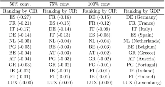
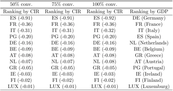
Figure 1 shows the time path of bank loan rates in the euro area together with that
of the policy rate. The bank loan rates are the ones for outstanding loans, lent from
banks to non…nancial businesses with contract lengths of up to one year.2 We see general
comovements between the bank loan rates and the policy rate, but, at the same time,
sizable dispersions in the bank loan rates across countries. Bank loan rates di¤er in their
1
Many existing studies show that the bank loan interest rate and the money market rate comove in the long run, but the former interest rate is sluggish compared with the latter interest rate in the short run; that is, bank loan rates adjust to the policy interest rate with some lags. See Mojon (2000), De Bomdtet al. (2002), Weth (2002), Gambacorta (2008), and De Graeveet al. (2007) for sticky bank loan rates in the euro area. Slovin and Sushka (1983) and Berger and Udel (1992) examine the short-run pass-through of US bank loans and conclude that there is a sizable stickiness in US bank loan rates. BOJ (2007, 2008) …nd similar results for Japanese banks. Mojon (2000) also discusses the possible causes of loan rate stickiness in the retail banking sector.
2
The data are taken from the harmonized national MFI interest rate statistics (MIR), released from the ECB. The series are available only from January 2003.
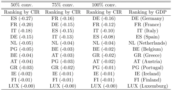
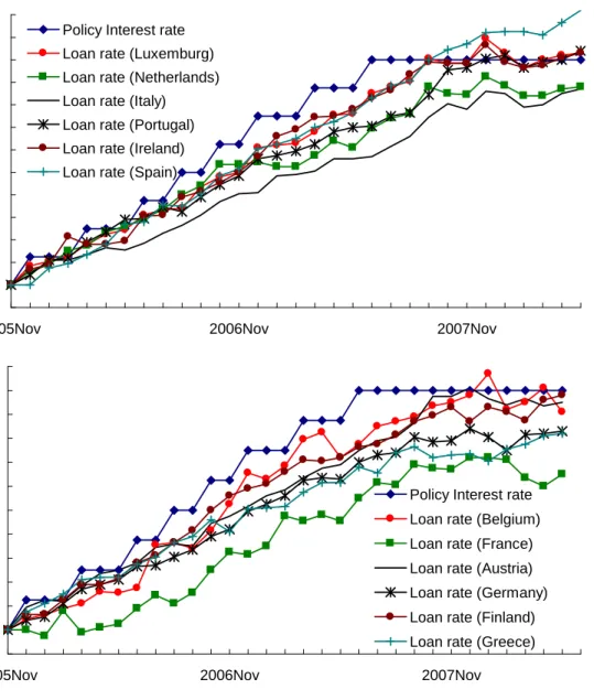
levels and in their dynamics. Figure 2 focuses more on the heterogeneity in the dynamics
and shows changes in the bank loan rates from November 2005.3 We con…rm that except
for a few countries, the bank loan rates increase following an increase in the policy rate
with di¤erent time lags.
In spite of a number of empirical studies on the heterogeneities of the bank loan rates,
theoretical investigations on …nancial market heterogeneity in the context of monetary
policy are still limited. In this paper, we incorporate heterogeneous features of the bank
loan rates into the New Keynesian framework to o¤er a tractable tool to investigate the
role of heterogeneous bank loan markets. We derive the optimal monetary policy under
heterogenous bank loan markets, thereby showing signi…cant changes in the way that
mon-etary policy is implemented. This is because the optimal response to particular loan rate
dynamics do not secure an optimal policy response to other loan rate dynamics because of
this heterogeneity.
The contribution of the paper can be summarized into four points below. First, we
empirically measure the levels and stickinesses of the bank loan rates in the euro area.
There are substantial cross-country di¤erences for both measures of the bank loan rates.
For the …rst measure, the levels of the bank loan rates vary re‡ecting the di¤erences in
loan rate markup from country to country, while the banks in the euro area refer to the
common policy rate. For the second measure, we examine the cross-country di¤erences in
stickinesses of the bank loan rates by estimating error correction model.
Second, we develop a New Keynesian model that captures the observed features of
the heterogeneity in the bank loan rates. We explicitly incorporate the banking industry
and the bank loan rate following Barth and Ramey (2000) and Ravenna and Walsh (2006).
Our framework, however, crucially di¤ers from Ravenna and Walsh (2006) in the bank loan
market structure. While complete markets are assumed in Ravenna and Walsh (2006), we
consider an economy where banks face monopolistic competition and friction associated
3
We subtract the bank loan rates at each period from their own levels in November 2005, the date one month before the ECB started to raise its policy rate.
with bank loan rate adjustment as in Teranishi (2008a). Moreover, banks are not identical
in their degree of nominal loan rate rigidity, the size of the loan rate steady-state markup,
and their share of the lending volume. In our model, the wedge between the loan rate
and the policy rate is due to the imperfect competition among banks following Sander
and Kleimeier (2004), Gropp et al. (2006), van Leuvensteijnet al. (2008) and Gropp and
Kashyap (2008) that show the importance of bank competitions on the staggered loan rate
setting and the loan rate markup.
Third, we analyze a structure of the optimal monetary policy rule in this economy
using a second-order approximated welfare function. Our welfare analysis reveals that the
central bank should take account of the several measures of heterogeneity in the bank loan
markets; i.e., credit spread between bank loan rates and the variations in each bank loan
rate. A central bank attaches weight to such measures according to the degree of bank
loan rate stickiness, the degree of the steady-state loan rate markup, and the size of the
loan market. With su¢ ciently large bank loan rate stickiness or a small steady-state loan
rate markup, a central bank should weight more heavily the variations in bank loan rates
rather than the credit spreads between them. Moreover, loan markets with larger loan rate
stickiness, with smaller steady-state loan rate markups, or with a larger share of lending
volume are given higher signi…cance by the central bank.
Fourth, using the results of the welfare analysis we quantitatively investigate the optimal
monetary policy in the euro area. With the estimated country-speci…c bank loan rate
stickinesses, the country-speci…c steady-state markups on the loan rates, and the …nancial
market share of the countries, the relative importance of each national bank loan market is
derived from the viewpoint of the optimal monetary policy. The monetary policy priority
ranking is not the same as the ordering according to the size of …nancial markets. As the
…nancial integration deepens, however, it is predicted that the ordering will converge to
those associated with the size of the …nancial markets.
The paper is organized as follows. Section 2 reports the size and diversity of the bank
describes our model with heterogenous banks. Section 4 analyzes the welfare implication
of the model. Section 5 is devoted to investigating the properties of the optimal monetary
policy. In Section 6, we calibrate the economy to the data from the euro area and illustrate
the optimal response of the ECB to the shock in the bank loan rates. Section 7 concludes.
2
Empirical facts about loan interest rates in the euro area
As discussed above, there is ample empirical evidence of the heterogeneity among the
bank loan rates in the euro area. There are level di¤erences among the loan rates, as
suggested by ECB (2008) and Gropp and Kashyap (2008), and the diversity in the loan
rate stickinesses, as suggested by Mojon (2000), Sørensen and Werner (2006), and van
Leuvensteijn et al. (2008). We focus on the fact that cross-country level di¤erences are
equivalent to the cross-country markup di¤erences of the bank loan rates and report the
ratio between the country-speci…c bank loan rates over the policy rate. For the loan rate
stickiness, we employ an error correction model, following Sørensen and Werner (2006).
Our data set contains monthly interest rate data on outstanding (stock) loans from
banks to enterprises, taken from MFI Interest Rate Statistics released by the ECB. The
sample period extends from January 2003 to May 2008. We have chosen the interest rates
on outstanding loans rather than the interest rates on new loans so as to be consistent
with our model.4 MFI Interest Rate Statistics provides time series data of the loan interest
rates for di¤erent lengths of loan maturity. We use loans up to one year.5
2.1 Heterogeneous loan rate markup
As we have noted above, the observed cross-country bank loan rates di¤er in levels as shown
in Figure 1. One of the reasons for the di¤erence in the loan rate level is that private banks
4
In the model, we assume that all the …rms’ expenses associated with their production is …nanced by borrowings from their banks. From this point of view, we consider that the interest rates on outstanding loans capture more of the important features of our model than the loan interest rates on the newly contracted loans. Moreover, because our model does not assume …nancial intermediation among households, we focus on the bank loan interest rate between banks and enterprises.
in di¤erent countries have di¤erent markups from the ECB’s policy rate to their loan rates.
For the bank loan rate in each country, we consider the time average of the ratio of the
bank loan rate over the policy rate, from January 2003 to May 2008, as the steady-state
loan rate markup. We assume that the steady-state loan rate markup is time invariant.
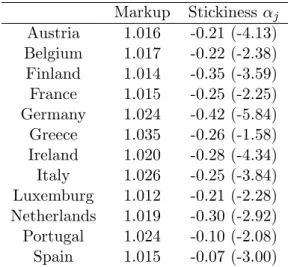
The second column of Table 1 shows the loan rate markup of each country. We see that
there is enough heterogeneity in the loan rate markup. For example, the markup on the
loan rate is much higher in Italy than in Finland.6 The markup in Italy is 2.6%, but it is
1.4% in Finland.
2.2 Heterogeneous loan rate stickiness
Not many studies focus on the diversity of the bank loan rate stickiness across countries.
Sørensen and Werner (2006) is one exception. Following Sørensen and Werner (2006), but
with an extended sample period, we estimate the country-speci…c loan rate stickiness for
12 euro countries.
Our error correction model is described as follows:
4Rbjt = j Rbjt cj jbit + p X k=1 jk4Rbjt k+ q X k0=1 'jk04bit k+ujt;
where Rbjt denotes the bank loan interest rate of country j,bit denotes the ECB’s policy
interest rate, and cj, j, j, jk, 'jk0 for k = 1; :::p and k0 = 1; :::q, are the estimated
country-speci…c parameters. We assume p = q = 2 for the estimations. Among the
estimated parameters, j governs the speed of the bank loan rate adjustment for country
j by which we assess the country-speci…c stickiness of the bank loan rates.
The third column of Table 1 reports coe¢ cients jfor euro countries, where the numbers
in parentheses are tvalues. The coe¢ cient j being closer to -1.0 indicates that the bank
loan rate of a countryjadjusts quicker to a change in the policy rate. The …rst observation
6From Subsection 2.2, we can estimate the markups byc
j and j. However, in this case, the markups
change according to the level of the policy interest rate. Thus, we use the average di¤erence as an average measure of the markups.
from the table is that for all the countries, the bank loan rates show some degrees of
stickiness. None of the coe¢ cients j is below -0.5. The second observation is that there
is a huge variety of loan rate stickiness across countries. For example in Germany, more
than 40% of the deviation from the long-run relationship is canceled in the next period,
while less than 10% of the deviation is canceled in Spain.
3
Model
Our model consists of …ve types of agents: two types of private banks, a consumer, …rms,
and a central bank. Banks …nance …rms’production by loan contracts. Existing studies of
the cost channel, including Ravenna and Walsh (2006), investigate a case where the bank
loan market is perfectly competitive. We assume that the bank loan market is
monopolisti-cally competitive and the loan interest rate contract is set under the Calvo pricing scheme
following Teranishi (2008a). The loan rates in our model are thus sticky compared with
the policy rate, as we observed from the data. Moreover, there are two types of loans, and
each of them is set by the di¤erent types of banks. The two types of loans are distinct in
their stickiness so that one loan rate adjusts quicker than the other does.
3.1 Demand for bank loans
We …rst describe how the volumes of the bank loans are determined in our model. Our
economy includes the two types of banks, two types of workers, and one type of …rm. Bank
loan contracts are made between the banks and the …rms. The loan contracts …nance the
…rms’expenses for hiring workers. The interest rates on the bank loans are determined by
banks in monopolistically competitive markets.
Private banks are di¤erentiated and categorized into the two types, depending on the
stickiness of their loan rates. The banks that provide more sticky loans populate overhM 2
[0; nM), and the banks that provide less sticky loans populate overhL2[0; nL]. We assume
that the sum of nM andnL is unity. We call the former typeM banks and the latter type
two types, type M workers and type L workers. Type M workers populate over hM 2
[0; nM), and typeL worker populate overhL2 [0; nL].
Firm f 2 [0;1] optimally hires both types of workers as price takers and sells the di¤erentiated …nal goods y(f) as a monopolistically competitive producer. The types of workers and bank loans are linked. In order to …nance the hiring cost of type M workers,
…rms need to borrow from a typeM bank. Similarly, in order to …nance the wages for type
L workers, …rms must borrow from type L banks. Firm f constructs the subcomposite
of labor inputs for each type of worker, which we denote by LM;t(f) and LL;t(f), and
aggregate them to Let(f).7 Firms employ both types of workers so that the two types of
bank loans are both tied to the …rm f.8 One way to think about this speci…cation is to
consider that the two types of business units associated with the labor types in the …rms
are …nanced by the di¤erent loans. Note that the private banks monopolistically compete
with each other both among the same type of bank and between the di¤erent types of bank
in our model.
The …rst step in the cost-minimization problem for …rmf with respect to the allocation
of type j worker, for j=L; M, is given by:
min
lj;t(hj;f)
Z nj
0
[1 +rj;t(hj)]wj;t(hj)lj;t(hj; f)dhj;
subject to the size of the subcomposite of typej labor input to …rmf,Lj;t(f):
Lj;t(f) " 1 nj 1 j Z nj 0 lj;t(hj; f) j 1 j dhj # j j 1 ;
whererj;t(hj)is the interest rate applied on the loan contract between …rmf and bank hj
in type jbanks, lj;t(hj; f)is the laborhj of typej workers hired by …rmf,wj;t(hj) is the
nominal wage for hiring the laborhj of typejworkers, and j is a preference parameter on
7
The same structure is assumed for employment in Woodford (2003). 8
In the current paper, we assume that …rms …nance all of their expenditure for their inputs by bank loans. Teranishi (2008a) relaxes this assumption and develops a setting where …rms …nance part of the production cost by loans.
di¤erentiated laborers. j governs both the wage markup and the markup from the policy
rate to the loan rate in our model.
The relative demand for workerlj;t(hj; f)is given as follows:
lj;t(hj; f) = 1 nj Lj;t [1 +rj;t(hj)]wj;t(hj) j;t j ; (1) where: j;t 1 nj Z nj 0 f [1 +rj;t(hj)]wj;t(hj)g1 jdhj 1 1 j : (2)
As a result, the total cost of hiring hj of typej workers for …rmf is expressed by:
Z nj
0
[1 +rj;t(hj)]wj;t(hj)lj;t(hj; f)dhj = j;tLj;t(f):
The two optimal conditions above ensure the optimal allocation oflj;t(hj; f) forj=M; L
with Lj;t(f) for j = M; L provided. For j = M; L; the …rm f’s optimal allocations
associated with Lj;t(f) are obtained by the second step of the cost-minimization problem
described below: min LM;t;LL;t X j=M;L j;tLj;t(f);
subject to the quantity of total labor input, which we assume as:
e Lt(f) Y j=M;L [Lj;t(f)]nj nnj j :
Then, the relative demand functions for each labor composite are derived as follows:
Lj;t(f) =njLet(f) j;t et 1 ; (3) where: et Y j=M;L nj j;t:
Using the relationships above, the following equations are obtained: M;tLM;t(f) + L;tLL;t(f) = etLet(f); (4) lj;t(hj; f) = [1 +rj;t(hj)]wj;t(hj) j;t j j;t et 1 e Lt(f); forj =M; L: (5)
Equation (4) denotes the cost share of each type of worker in the total cost expenditure
of …rm f: etLet(f) stands for the total cost, and j;tLj;t(f) stands for the cost of hiring
type j workers. Equation (5) indicates the demand function for the di¤erentiated labor
input lj;t(hj; f): Note that the demand for each di¤erentiated worker depends on wages
wj;t(hj), loan interest rates rj;t(hj), and the relative price of the subcomposite of labor
input j;t, given the total demand for laborLet(f).
Finally, we can derive the demand function for bank loans associated with hiring of
di¤erentiated labor hj of typej, borrowed by …rm f as follows:
qj;t(hj; f) = wj;t(h)lj;t(hj; f) = wj;t(hj) [1 +rj;t(hj)]wj;t(hj) j;t j j;t et 1 e Lt(f); forj=M; L:
This condition demonstrates that the demand for each di¤erentiated loan qj;t(hj; f)
de-pends on the wages, loan interest rates, and relative price of the labor subcomposite given
the total labor demand. With the two-step cost minimization, the private banks
monopo-listically compete both against the same type of bank and between the two di¤erent types.
For aggregate labor demand conditions, we obtain following expression:
e Lt= Z 1 0 e Lt(f)df: 3.2 Consumer
A representative consumer derives utility from consumption, and disutility from the supply
U Tt=Et 8 < : 1 X T=t T t 2 4U(CT) X j=M;L Z nj 0 V(lj;T(hj))dhj 3 5 9 = ;;
where Etis an expectation conditional on the state of nature at datat. The functionU and
V are increasing and concave in the consumption index and the labor supply, respectively.
The budget constraint of the consumer is given by:
PtCt+Et[Xt;t+1Bt+1] +Dt Bt+ (1 +it 1)Dt 1 (6) + X j=M;L 1 j Z nj 0 wj;t(hj)lj;t(hj)dhj + Bt + Ft +Tt;
whereBtis a risky asset, Dtis the amount of bank deposits, j is the tax for wage income,
Tt is the lump-sum tax, anditis the nominal deposit rate set by a central bank from tto
t+ 1. B
t =
R1
0 Bt 1(h)dh is the nominal dividend stemming from the ownership of the
banks, Ft = R01 Ft 1(f)df is the nominal dividend from the ownership of the …rms, and
Xt;t+1 is the stochastic discount factor. We assume a complete …nancial market for risky
assets. Thus, we can hold a unique discount factor and can characterize the relationship
between the deposit rate and the stochastic discount factor as:
1 1 +it
=Et[Xt;t+1]: (7)
We assume that the household has Dixit–Stiglitz preferences (Dixit and Stiglitz, 1977),
where aggregate consumption Ct is linked to the di¤erentiated goods ct(f)produced by a
…rm f 2[0;1]by the following equation:
Ct Z 1 0 ct(f) 1 df 1 ;
where >1is the elasticity of substitution across goods. The aggregate consumption-based
Pt Z 1 0 pt(f)1 df 1 1 ;
where pt(f) is the price of di¤erentiated good ct(f). The demand function for ct(f) is
derived from the cost-minimization behavior of the consumer as:
ct(f) =Ct
pt(f)
Pt
: (8)
Given the optimal allocation of consumption expenditure across the di¤erentiated
goods, the consumer must choose the total amount of consumption, the optimal amount
of risky assets to hold, and an optimal amount to deposit in each period. Necessary and
su¢ cient conditions are given by:
UC(Ct) = (1 +it)Et UC(Ct+1) Pt Pt+1 ; (9) UC(Ct) UC(Ct+1) = Xt;t+1 Pt Pt+1 :
Equations (7) and (9) express the intertemporal optimal allocation on aggregate
consump-tion. Assuming that the goods market clears for allf 2[0;1], the standard New Keynesian IS curve is derived by log-linearizing equation (9):
xt=Etxt+1 (bit Et t+1); (10)
where xt and t+1 are the output gap and in‡ation, respectively. The de…nition of the
output gap is given in the next subsection. We usembtto denote the percentage deviation
of the variablemt around the nonstochastic steady state. is de…ned by UUY
Y YY >0.
A consumer provides di¤erentiated types of labor to …rms, holding the power to decide
the wage of each type of labor as assumed in Erceget al. (2000). Given the labor demand
in every period to maximize its utility subject to the budget constraint (6).9 This yields
the following relations for the type j worker:
wj;t(hj) Pt = 1 j j j 1 Vl[lj;t(hj)] UC(Ct) : (11) 3.3 Firms
Given the cost of hiring labor inputs eTLeT (f)discussed above, …rms set the price of their
products optimally. We assume that …rms face a monopolistically competitive market as in
Calvo (1983) and Yun (1996) (henceforth Calvo-Yun setting). That is, facing
downward-sloping demand curves, …rms set di¤erentiated goods prices in a staggered manner a la
Calvo-Yun setting.
A …rmf 2[0;1]maximizes the present discounted value of pro…t, which is given by:
Et 1 X T=t T tX t;T h pt(f)yt;T(f) eTLeT(f) i ; (12)
where(1 )is the probability that the …rm can reset its price. We assume the production
function of the …rm f as yt(f) = F(LeT(f)), where F() is increasing and concave. The
Dixit–Stiglitz preferences implies that equation (12) can be written as:
Et 1 X T=t T tX t;T ( pt(f) pt(f) PT CT eTLeT (f) ) :
The optimal pricespt(f) set by the active …rms are given by:
Et 1 X T=t ( )T tUC(CT) PT yt;T(f) " 1 pt(f) eT @LeT (f) @yt;T(f) # = 0; (13)
where we substitute equation (8). Further substituting equation (11) into equation (13)
9
In contrast to Erceg et al. (2000), however, we assume no sticky wages so that the consumers can change their wages in every period.
leads to: Et 1 X T=t ( )T tUC(CT)yt;T(f) 1pt(f) Pt Pt PT M M 1 nM L L 1 nL Zt;T(f) = 0; (14) where: Zt;T(f) = Y j=M;L 8 < : 1 nj Z nj 0 [1 +rj;t(hj)]1 j ( Vl[lj;T(hj)] UC(Ct) @Let;T(f) @yt;T(f) )1 j dhj 9 = ; nj 1 j :
By log-linearizing equation (14), we derive:
1 1 pbet(f) =Et 1 X T=t ( )T t " T X =t+1 H; +nMRbM;T+nLRbL;T +mcct;T(f) # : (15)
We de…ne the real marginal cost as:
c mct;T(f) X j=M;L Z nj 0 c mcj;t;T (hj; f)dhj; where: mcj;t;T(hj; f) Vl[lj;T(hj)] UY (CT) @Let;T(f) @yt;T(f) forj =M; L:
We also de…ne forj =L; M:
Rj;t 1 nj Z nj 0 rj;t(hj)dhj; (16) e pt(f) pt(f) Pt and t Pt Pt 1 :
Then, equation (15) can be transformed into:
1 1 pbet(f) =Et 1 X T=t ( )T t " (1 +!p ) 1 mccT +nMRbM;T +nLRbL;T + T X =t+1 # ; (17)
where we make use of the relationship: c mct;T(f) =mccT !p " be pt(f) T X =t+1 # ;
where!p is the elasticity of @
e
Lt;T(f)
@yt;T(f) with respect toy. We further denote the average real
marginal cost as:
c mcT X j=M;L Z nj 0 c mcj;T (hj)dhj; where for j=M; L: mcj;T(hj) Vl[lj;T(hj)] UY (CT) @LeT @YT :
The point is that the unit marginal cost is the same for all …rms because each …rm pays for
all the types of labor and associated loans with the same proportion. Thus, all the …rms
set the same price if they have a chance to reset their prices at timet.
In the Calvo-Yun setting, the aggregate price indexPt evolves by:
Pt1 = Pt1 1 + (1 ) (pt)1 ; (18) where: Pt1 Z 1 0 pt(f)1 df and p1t Z 1 0 pt(f)1 df:
Log-linearizing equation (18) and equation (17) leads to the following New Keynesian
Phillips curve:
t= mcct+nMRbM;t+nLRbL;t + Et t+1; (19)
where the slope coe¢ cient (1 (1+)(1! )
p ) is a positive parameter. The equation is similar
to the standard New Keynesian Phillips curve, but it contains the terms associated with
the loan interest rates.
Here, according to the discussion in Woodford (2003), we de…ne the natural rate of
output Yn
1 = Y j=M;L j j 1 nj 1 +Rj nj 8 > < > : 1 nj Z nj 0 8 < : Vl h lnj j;t(hj) i UC(Ct) @Lent (f) @Yn t (f) 9 = ; 1 j dhj 9 > = > ; nj 1 j ;
where we assume a ‡exible price setting, pt(f) =Pt, and assume no impact of monetary
policy,rL;t(hL) =rM;t(hM) =R, and so holdyt(f) =Ytnunder the natural rate of output.
lnj
j;t(hj)forj=L; M andLent (f) are the amount of labor corresponding toYtn, respectively.
Then, we have:
c
mct= (!+ 1)(Ybt Ybtn);
where Ybt ln(Yt=Y), Ybtn ln(Ytn=Y), and ! is the sum of the elasticity of the marginal
disutility of work with respect to output increase and the elasticity of F0(F11(y)) with
respect to output increase.10 Then, by de…ningxt Ybt Ybtn, we …nally have:
t= xt+ nMRbM;t+nLRbL;t + Et t+1; (20)
where (!+ 1).
3.4 Private banks
The pricing strategy for the private banks is described in this subsection. Two types of
banks collect deposits from consumers at the interest rate 1 + i, and each bank hj of
type j 2 [M; L] makes bank loan contracts of volume qj;t(hj; f) for …rm f. The loans
are di¤erentiated and supplied in a monopolistically competitive manner. The banks are
subject to a nominal rigidity in adjusting their bank loan rates. We assume that bank hj
1 0! !
p+!w, where!w is the elasticity of marginal disutility of work with respect to output increase
in Vl(lt(h); t)
of type j can reset loan rates with probability 1 'j following the Calvo-Yun setting.
Bank hj of type j chooses the loan interest rate rj;t(hj) to maximize the present
dis-counted value of pro…t:
Et
1 X
T=t
'j T tXt;Tqj;t;T (hj; f)f[1 +rj;t(hj)] (1 +iT)g:
The optimal loan rate condition is now given by:
Et 1 X T=t 'j T t Pt PT UC(CT) UC(Ct) qj;t;T(hj)f[1 +rj;t(hj)] jf[1 +rj;t(hj)] (1 +iT)gg= 0: (21)
Because the active banks set the same loan interest rate, the aggregate loan interest rate
indexRj;t evolves as follows:
1 +Rj;t='j(1 +Rj;t 1) + 1 'j (1 +rt): (22)
Log-linearizing equations (21) and (22) gives the following loan rate curve for the type j
banks: b Rj;t = j1EtRbj;t+1+ 2jRbj;t 1+ j3bit; (23) where j1 'j 1+('j)2 , j 2 'j 1+('j)2 , and j 3 1 'j 1+('j)2 j j 1 (1 'j)(1+i) 1+Rj for j = M; L are all positive.
Finally, the market clearing conditions for bank loansj forj=M; L are:
qj;t;T(hj) = Z 1 0 qj;t;T(hj; f)df ; Z nj 0 qj;t;T(hj)dhj =njDT forj =M; L: 3.5 System of equations
The linearized system of equations consists of …ve equations: (10), (20), (23), and an
,bi,RbM, and RbL.
4
Optimal monetary policy with heterogeneous loans
4.1 Approximated welfare functionIn this section, we derive a second-order approximation to the welfare function following
Woodford (2003). The detail of derivation is shown in Appendix A.
Consumer welfare is given by:
E0 1 X t=0 tU T t=E0 ( 1 X t=0 T t U(C t) Z nM 0 V(lM;t(hM))dhM Z nL 0 V(lL;t(hL))dhL ) :
Then, we have a second-order approximated loss function expressed as follows:
E0 1 X t=0 tU T t' E0 1 X t=0 t 0 @ 2 t + x(xt x )2+ M L RbM;t RbL;t 2 + M RbM;t RbM;t 1 2 + L RbL;t RbL;t 1 2 1 A; (24)
where , x, M, L, and M L are positive parameters.11
It is important to note that equation (24) indicates that the central bank should take
account of the heterogeneity in the bank loan market as well as the aggregate variables
such as in‡ation rate t and the output gapxt. The central bank minimizes the variations
of each bank loan rate, the last two terms in equation (24), and the credit spread between
them, the third term in equation (24). Apart from the aggregate variables, the relative
signi…cance among them depends on the sizes of j forj =M; Land M L. Because of the
heterogeneity in the …nancial market, the stabilization policy for one loan rate acts as the
destabilization policy for another loan rate. This is a trade-o¤ in the …nancial market in
conducting monetary policy. Details of this trade-o¤ are discussed in the next subsection.
For illustrative purposes, consider an economy where bank types are homogenous, where
only one type of loan is available, so that their loan interest rates respond to a policy
1 1
Note that we assuem the wage tax as 1
j =
j
j 1
2
to realizelL(hL) =lL(hL) =Lefrom an optimization
interest rate uniformly. Then it is the case that RbM;t=RbL;t=Rbt and M = L= , and
the loss function is reduced to:
1 X t=0 tU T t' 1 X t=0 t 2 t+ x(xt x )2+ Rbt Rbt 1 2 : (25)
In this equation, neither the credit spread term nor the term of the heterogeneous bank loan
variations is present. No trade-o¤ regarding the …nancial market emerges in conducting
the monetary policy. Comparing this economy, the optimal monetary policy becomes more
complicated in an economy with heterogenous banks.
4.2 Priority in monetary policy
With heterogenous banks, an optimal response to a cost shock in one loan interest rate
curve does not secure an optimal response to another loan interest rate curve. Thus, there
is a clear trade-o¤ in conducting the optimal monetary policy, and a central bank needs to
determine the ordering among the bank loan curves.
To see this point, consider a response of a central bank to a cost-rise shock that hits
the bank loan rate. We assume that the shock uj;t enters in the laws of motion for the
bank loan rates curve in the following way:
b
Rj;t= j1EtRbj;t+1+ j2Rbj;t 1+ j3bit+uj;t forj=M; L:
For illustrative purposes, we assume that uM;t and uL;t are not correlated.
Before showing details of the simulation, we analytically demonstrate the trade-o¤ in
the …nancial market. When we observe a positive idiosyncratic shock uM;t >0 (uL;t= 0)
in the bank loan market of typeM; equation (24) leads to a decline in the policy interest
ratebit;so as to accommodate uM;t: It, however, operates as a disturbance in the type L
bank loan curve. In particular:
(RbM;t RbM;t 1)2= n 1 M1 F M2 L (1 L) h M 3 bit+uM;t io2 ;
(RbL;t RbL;t 1)2= n
1 L1F L2L (1 L)h L3bit
io2
:
The equations illustrate the trade-o¤ originating from the central bank’s welfare function.
As we see in equation (24), a central bank adjusts its policy rate to a shock in the bank
loan rate curve so as to reduce the LHS of these equations. We learn from the …rst equation
that a central bank lowers the policy rateitin order to o¤set the variations caused byuM;t.
Loweringbit, however, leads to larger variations in the LHS in the second equation. The
relative signi…cance of those two LHSs is dependent on the welfare weight j forj=M; L.12
It should be noted that even for the common shock,i.e.,uM;t=uL;t6= 0, there is a trade-o¤
in conducting monetary policy when the heterogeneous bank loan markets are present.
In this subsection, we quantitatively investigate the relative signi…cance of each term
that appears in the equation above. As we discussed above, the banks in the current model
di¤er from each other in terms of three parameters: the degree of loan rate stickiness 'j,
the size of the steady-state loan rate markup j
j 1, and the …nancial market sharenj of the
lending volume. We consider the commitment of optimal monetary policy under a timeless
perspective in the sense of Woodford (2003).13 Appendix B shows the optimal targeting
rule in this model. For the parameterization on the stickiness of the bank loan rates, we
follow the results obtained in Slovin and Sushka (1983). From the time series analysis of
the US commercial loans, they obtain that, on average, bank loan rates need at least two
quarters and perhaps more to adjust to a change in the market interest rate. Thus we
set the average contract duration of less sticky loan interest rates RL;t as 'L = 0:5 (two
quarters) and set'M = 0:6for the more sticky loan interest rateRM;t. Other parameters
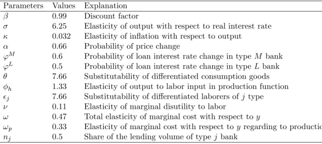
are borrowed from Rotemberg and Woodford (1997), and reported in Table 2.
1 2
As we discussed in the previous section, when the bank loan rates are nearly ‡exible, the response of the central bank to the credit spread shock is ambiguous because of the credit spread term. This point is summarized in Teranishi (2008b) in terms of the spread-adjusted Taylor rule.
1 3
In this setting, as shown in Woodford (2003), the central bank conducts the monetary policy in a forward-looking way by paying attention to future economic variables and by taking the e¤ect of the monetary policy on those future variables into account.
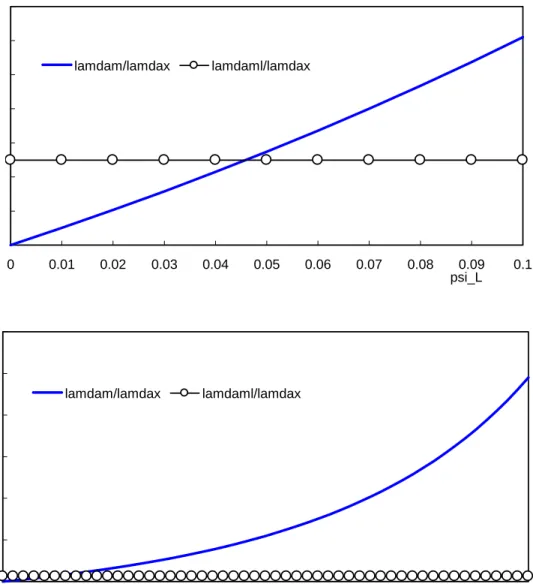
4.2.1 Sensitivity to loan rate stickiness
Figure 3 reports the values of relative weights L x and
M L
x for various sizes of bank loan
rate stickiness 'L.14 The upper panel displays the case when 'L is su¢ ciently small,
and the lower panel shows the case when 'L is large. It is clear from the …gure that
the welfare weight on the variation in the bank loan rate set by the type L bank, L x, is
monotonically increasing in 'L, while M L
x is invariant to changes in '
L. A reason for
this monotonic increase is that higher stickiness of the loan rate leads to larger dispersion
among labor inputs when a shock hits the economy. Our welfare function indicates that
higher labor dispersion is tied to lower quantity of goods production accompanied by lower
utility from consumption and higher labor disutility.15 When the bank loan interest rate
'L is su¢ ciently small, the prime concern for the central bank is the spread between the
more sticky bank loan rate and the less sticky bank loan rate rather than the variations
of each bank loan rate. As 'L becomes larger, it is more relevant for the central bank to
concentrate on the variations of the individual loan rate rather than the spread.
As we will see below, for all the countries in the euro area, the estimated size of the bank
loan rate stickiness'J is far above the level under which the credit spread term has a larger
signi…cance for the central bank. The same is true for other developed countries, such as
the US (Slovin and Sushka, 1983; Berger and Udell, 1995) and Japan (BOJ, 2007; BOJ,
2008). Therefore, in implementing monetary policy in the current environment, a central
bank should attach higher weight to the variations of the loan interest rates in bank loan
markets. Our results for the credit spread term have, however, important implications for
the future. Existing studies about the banking sectors agree with the view that bank loan
rate stickiness is diminishing. For example, Ito and Ueda (1981), Sander and Kleimeier
(2004), Groppet al. (2006), and van Leuvensteijnet al. (2008) argue that the deregulation
of bank loan markets accompanied by higher competition among banks leads to lower loan
rate stickiness. Thus, with a competitive …nancial market, a central bank should pay more
1 4
attention to the credit spread rather than the variation in bank loan rates.
Figure 4 illustrates the simulation where we impose idiosyncratic shocks on the bank
loan interest rate curves. We assume a unit cost rise for the bank loan rates, uj with
persistence of 0.9. In the upper panel, we show the impulse responses of the policy rate and
the bank loan rate set for two types of banks, to a positive shock in the typeM loan interest
rate,uM, maintaininguL= 0. Similarly, the lower panel displays the impulse responses of
the variables to a positive shock in the type LloanuL, maintaininguM = 0. Two features
are observed from the panels. First, even with the trade-o¤ problem originating from the
heterogeneity of the loan interest rate stickiness, the central bank lowers the policy rate
when a positive shock hits the economy.16 Second, a central bank lowers the policy rate
more in response to a shock in a type M bank loan rate than to a shock in a typeL bank
loan rate. The larger monetary easing implies a larger weight on the bank loan markets hit
by the shock because it induces a smaller positive response in the loan rate that is directly
hit by the shock but a larger negative response in the loan rate that is not directly hit
by the shock. This is a trade-o¤ to the …nancial market in conducting monetary policy.
The simulation result shows that the central bank should put its monetary policy priority
on the more sticky loan rate dynamics than the less sticky loan rate dynamics, even when
the same size shocks hit the economy. As we discussed above, one reason for this is that
the welfare weight increases as the loan rate stickiness increases. The central bank has
an incentive to avoid a large ‡uctuation in bank loans with a higher j. Another reason
is that the same size shock creates a larger ‡uctuation in the loan rate curve with more
stickiness because the inertia in the loan interest rate dynamics increases as the loan rate
stickiness increases in the loan rate curves.17
1 6This optimal monetary policy response to a shock in the bank loan interest rate curve is consistent with the actual behavior of the central banks. For example, the FRB has lowered the policy interest rate in the subprime mortgage crisis from the fall of 2007, in order to mitigate the rise in the premium (see Taylor, 2008).
4.2.2 Sensitivity to steady-state markup from policy rate to loan rate
Figure 5 reports the values of relative weights L x and
M L
x for various sizes of bank loan
rate stickiness 'L, changing the size of L. Because the steady-state markup is LL1,
this parameter governs a markup from the policy rate to the loan rate. As L increases
(the labor di¤erence decreases), the steady-state markup decreases. As the degree of the
steady-state markup decreases, the weight of L
x increases. M L
x , however, does not change
with the steady-state markups. We can think of the same reason in the relation between
L
x and '
L as discussed above. In economic shocks associated with the loan rate, smaller
di¤erences in labor, i.e.,higher j, yield a larger substitution e¤ect among loans and lead
to higher economic ‡uctuations. In other words, we interpret this point as indicating that
greater similarity among businesses increases loan rate ‡uctuations to the shocks thanks to
high substitution among loans in the loan demand function. Then, a smaller steady-state
markup induces both more labor disutility and more production dispersions associated
with more disutility from consumption to the shocks. Moreover, the importance of the
credit spread decreases as the size of the steady-state markup decreases. As shown in
later sections, for all the countries in the euro area, the estimated size of the steady-state
markup is above the level under which the credit spread term becomes more important to
the central bank.
Figure 6 illustrates the simulation where we impose idiosyncratic shocks on the bank
loan market with di¤erent steady-state markups. We assume an asymmetric degree of
labor di¤erence such that M = 7:66 and L = 10. Thus, the steady-state markup on the
loan rate is larger in bank loan M than in bank loan L. For illustrative purposes, we set
a symmetric situation except for j as 'j = 0:6 and nj = 0:5 for j = M; L. We impose
these shocks and show the results. First, even under the presence of the trade-o¤ problem
because of heterogeneity in the steady-state markup, the central bank lowers the policy rate
when the shock hits the economy. Second, a central bank lowers the policy interest rate
more in response to the shock in the smaller steady-state loan rate markup,i.e. less labor
Thus, the central bank should put its monetary policy priority on the loan rate with the
smaller steady-state markup rather than that with the larger steady-state markup for the
same size shock. The reason for this is that the weight in the welfare function increases as
the steady-state markup in the interest rate decreases as implied in Figure 5. Note that
the markups associated with j capture the banks’ markups at the steady state. Thus,
in our model, the central bank can a¤ect the variation in the loan rate around its steady
state through monetary policy, but it cannot alter the markup in the steady state itself.
Our view is in line with that of Adam et al. (2002). They stress the importance of the
institutional di¤erences in accounting for the loan rate di¤erences across countries.
Cross-country heterogeneity in the tax systems and legal systems is present in the euro area
after 1999, and the related coordination has progressed only gradually (Adamet al., 2002).
Those factors are beyond the in‡uence of monetary policy. We consider an economy where
the central bank concentrates on the loan rate dynamics, taking the size of the markup at
the steady state as exogenously given. Under this environment, it is optimal for the central
bank to attach higher weight to the loan rate variations with a smaller steady-state loan
rate markup than to those with a larger steady-state loan rate markup.
4.2.3 Sensitivity to market share
Figure 7 reports the values of relative weights L x and
M L
x for various levels of bank loan
interest rate stickiness 'L, with a changing market share of loans nL. We see that Lx
increases as nL increases. This is just because the impact of the loan market L from the
shock to the economy increases because the market share of the loan M increases. M L x
takes the maximum value at nL = 0:5, and it decreases as nL moves away from 0.5 (see
Appendix A for details).
Figure 8 illustrates the simulation where we impose idiosyncratic shocks on the bank
loan market with a larger share of bank loan typeL,i.e.,nL= 0:8, in a symmetric situation
with'j = 0:6and j = 7:66 forj=M; L. Two observations should be noted. First, under
the central bank lowers the policy rate when the shock hits the economy. Second, a central
bank lowers the policy rate more in response to the shock in the loan rate with the larger
share than to the shock in the loan rate with the smaller share. Thus, the central bank
should put its monetary policy priority on the loan rate with the larger market share rather
than that with the smaller market share. One reason for this is that the weight on the
more sticky loan in the welfare function increases when nL increases as shown in Figure
7.18 Another reason is that banks with a higher market share have a greater e¤ect on the
economic dynamics as shown in equation (20). This implies that the market share, i.e.
the impact of the share on the economic dynamics, is also an important element in the
determination of monetary policy.
5
Monetary policy in the euro area
In this section, we conduct numerical analyses using the euro area data. Our model is very
suitable for an analysis of …nancial integration because the model includes the international
competition among heterogeneous banks that is a key element in the …nancial integration
in the euro area. The arguments about di¤erent bank types hold exactly for those banks
with distinct country-speci…c loan rate stickiness and steady-state markups on the loan
rate. As we have seen earlier, the cross-sectional heterogeneity in both the bank loan rate
stickiness and steady-state markups on the loan rate remains observable even a decade after
the debut of the new currency. The optimal monetary policy for a central bank is then
formulated distinctively given the observed size of bank loan stickiness for each country,
the size of steady-state markup on the loan rate for each country, and the size of their
…nancial markets.
5.1 Optimal monetary policy in the euro area
We …rst provide the relative signi…cance of each country, i.e.,the current monetary policy
current euro area data. The ECB responds di¤erently to each country shock as member
countries di¤er in their bank loan stickiness, their steady-state markup on the loan rate,
and their market size. We set the parameter values for the euro area as follows. The main
parameters = 0:72, = 6, and = 0:91 are from Smets and Wouters (2003).19 The other parameters are reported in Table 2. For the loan stickiness for each country, we
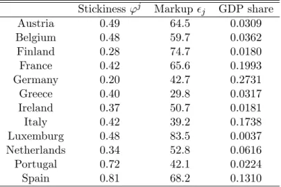
calculate the Calvo parameter from our estimation result in Table 1. For the steady-state
markup on the loan rate, we also use the values in Table 1. Table 3 provides the Calvo
parameters'j corresponding to the estimated stickinesses in Table 1 and j corresponding
to the estimated markup in Table 1.20 j belongs to one of 12 countries. We maintain the
two-types bank analysis used earlier. We divide the euro area into country j and the rest.
The lending volume nj for country j is set according to the GDP share of the country in
the euro area as in Table 3.21 The bank loan stickiness 'R, where R denotes the rest of the euro area, and the markup for the rest R
R 1 are calculated by the weighted average
of those parameters of the 11 countries in the euro area other than country j using their
GDP as weights.
In the simulation, we calculate the time path of the policy rate in response to a positive
innovation in the bank loan rate in country j. We measure the ordering of country j by
the size of the policy rate response to a country-speci…c shock in the loan rate in country
j relative to the other countries. A larger response of the policy rate to the shock for
country j indicates higher signi…cance of the bank lending channel of country j for the
central bank. As shown above, the bank loan rate stickiness'j, the steady-state loan rate markup on the loan rate j
j 1, and the share of lending volumenj play an important role
1 9We pick these values from the means in Table 1 of Smets and Wouters (2003). For calculation of , we assume that the consumption habit is zero.
2 0
We use the transformation:
'j= 1 x;
wherexis the absolute values in the …rst and second lines in Table 1. Then we change this monthly value to a quarterly value.
2 1
In the third column of Table 3 below, we show the GDP share of each euro country, based on the 2006 GDP series in the Total Economy Database, released by The Conference Board and Groningen Growth and Development Centre.
in our model.
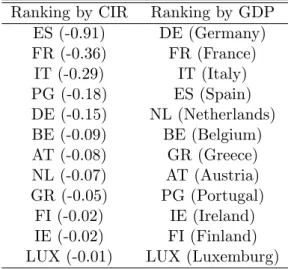
Figure 9 shows the impulse responses of the policy rate to a positive innovation in
the bank loan rate in each country. In response to the innovations, the central bank
lowers the policy rate, but the size of the decline in the policy rate di¤ers across countries.
Table 4 reports the cumulative impulse responses (denoted as CIR in the table) of the
policy rates and size of GDP for 12 countries by ranking. The numbers in parentheses are
the cumulative impulse response values. More negative values in the cumulative impulse
response indicate that the central bank responds more to the shock originated from the
country. An important implication of this simulation is that the ECB includes inequality,
which is not captured by the …nancial market sizes, in its monetary policy priorities under
imperfect …nancial integration.
5.2 Optimal monetary policy toward perfect …nancial integration
Another important feature is the ongoing processes of integration. While several studies
including Adamset al. (2002) and Gropp and Kashyap (2008) stress the prominent delays
of …nancial integration in the bank loan market, several legislative initiatives have been
conducted by the ECB membership countries to unify truly the euro loan market.22
Empir-ical studies, such as Mojon (2000) and van Leuvensteijnet al. (2008), indicate some degree
of convergence in the bank loan market. We show several possible scenarios associated the
…nancial integration in the euro area and o¤er a description of the optimal monetary policy
in each stage.
One plausible view on bank loan market convergence in the next decade is that
cross-country heterogeneity of the bank loan market may become less prominent. Mojon (2000)
argues that as a consequence of integration of the money market, the presence of alternative
ways to …nance investments makes the banks exposed to a higher degree of competition.
More severe competition brings homogenous and faster responses of the cross-country bank
2 2
For example, the 2nd Banking Directive of 1989 legally permitted the establishment of subsidiaries and branches of any bank residing in the EU in any other EU countries (Gropp and Kashap, 2008).
loan rates to the policy rate.23 Gropp and Kashyap (2008) imply that banks’markups on
the loan rates decrease as the competition in the loan market increases. This study suggests
that bank loan rates respond to the policy rate quicker in a homogenous manner and the
steady-state loan rate markup becomes smaller in all countries, as the bank loan markets
approach perfect …nancial integration where we assume that strong bank competition exists.
First, we consider a scenario in which the bank loan stickinesses of all countries approach
that of Germany, which has the lowest stickiness in the bank loan rate. For a given size of
the bank loan stickiness 'jdata for country j, we use the di¤erence in stickiness from that
of Germany'Germanydata as a measure of the degree of …nancial integration. We conduct this
hypothetical exercise by changing the di¤erence in the country-speci…c bank loan stickiness
relative to that of Germany.
Table 5 displays the cumulative impulse response (denoted as CIR in the table) of the
policy rate to a shock in the loan rate at various levels of the …nancial integration. The
numbers in parentheses are the cumulative impulse response values. The second column
indicates the cumulative impulse response and the monetary policy priority ranking of the
countries when'j = 'jdata 'Germanydata +'Germanydata with = 0:5. When = 0:5, the
distance between the country-speci…c bank loan stickiness and that of Germany by 50%.
The third and fourth columns report the case when = 0:25and = 0, respectively. It is
shown in the table that the priority ranking of the countries for a central bank changes in
each stage of the …nancial integration. Moreover, the ranking does not converge to that by
the …nancial market share of each country because of the heterogeneity of the steady-state
markup on the loan rate. Therefore, the steady-state markup on the loan rate as well as
the loan rate stickiness are also very important factors for the ECB in conducting monetary
policy.
Second, we consider a scenario in which the levels of steady-state markups on the
loan rates of all countries approach that of Luxemburg, which has the lowest steady-state
2 3
Using data from the euro area, van Leuvenstijn et al. (2008) shows that higher bank competition on the interest rate induces larger pass-through of the policy interest rate to the loan rates.
markup on the bank loan rate as before. Table 6 displays the cumulative impulse response
(denoted as CIR in the table) of the policy rate to a shock in the loan rate at various levels
of …nancial integration. The numbers in parentheses are the cumulative impulse response
values. The second column indicates the cumulative impulse response and the monetary
policy priority ranking of the countries when j = j data
Luxemburg
data +
Luxemburg data
with = 0:5. The third and fourth columns report the case when = 0:25 and = 0,
respectively. Regardless of the value of , the monetary policy priority does not change.
The outcomes, however, show that the ranking does not converge to that by the …nancial
market share of each country because of the heterogeneity of the loan rate stickiness. We
con…rm that the loan rate stickiness and the steady-state loan rate markups are both
important factors for the ECB.
Third, we consider a scenario in which both the levels of the steady-state markups on
the loan rates and the loan rate stickinesses of all countries approach those of Germany
and Luxemburg, respectively, as before. Table 7 shows that the ranking …nally converges
to the ranking by the …nancial market share of each country without the heterogeneity in
both the loan rate stickinesses and the steady-state markups on the loan rates.
6
Concluding remarks
We developed a New Keynesian dynamic stochastic general equilibrium model under the
imperfect …nancial integration,i.e.,cross-country di¤erences in the loan rate stickiness and the markup from the policy rate to the loan rate, within a single currency area. We then
investigated the optimal monetary policy rule under such an environment. We also carried
out the welfare analysis, indicating that the central bank needs to take account of the
heterogeneities in the bank loan markets, such as the size of the bank loan rate stickiness,
the level of the steady-state markup, and the share of the market in the bank loan market.
We calibrated our model using data from the euro area and computed the monetary
the size of the …nancial markets. As …nancial integration deepens further, however, it is
predicted that the share of the bank lending will become the only relevant measure in
implementing the optimal monetary policy.
The analysis in this paper suggests several directions for future research. It would be
of interest to examine the role of other types of heterogeneity across the di¤erent types
of interest rates. In particular, previous studies report the prominent di¤erence between
the bank loan rates and market interest rates in terms of their stickinesses. In this paper,
we concentrated on the di¤erence within the bank loan rates across countries in the euro
area. However there is ample evidence that …rms directly …nance their funds from the
…nancial market. The extension of our model, in this direction, enabled us to analyze
monetary policy in an economy where …rms can substitute between borrowing from the
banks and issuing corporate bonds. As suggested by Taylor (2008), we can also examine
the heterogeneity in interest rates between a risk-free asset, such as government bonds,
and a risky asset, such as commercial paper, in our framework. A model that captures
this heterogeneity may be important to understand better the transmission mechanism of
References
[1] Adam, K., T. Jappelli, A. Menichini, M. Padula and M. Pagano. “Analyse, Compare,
and Apply Alternative Indicators and Monitoring Methodologies to Measure the
Evo-lution of Capital Market Integration in the EU,”a study comissioned by the European
Commission, January, 2002.
[2] Baele, L., F. Annlise, P. Hordahl, E. Krylova, C. Monnet. “Measuring Financial
Inte-gration in the Euro Area,”ECB Occasional Paper No. 14, 2004.
[3] Bank of Japan. “Financial System Report,”Reports and Research Papers, March 2007.
[4] Bank of Japan. “Financial System Report,”Reports and Research Papers, March 2008.
[5] Barth M. J and Ramey V. A. “The Cost Channel of Monetary Transmission,”NBER
Working Paper Series 7675, 2000.
[6] Berger, A. and G. Udell. “Some Evidence on the Empirical Signi…cance of Credit
Rationing,”Journal of Political Economy, Vol. 100, 1992, pp 1047–1077.
[7] Berger, A. and G. Udell. “Small Firms, Commercial Lines of Credit, and Collateral,”
Journal of Finance, Vol. 68, 1995, pp 351–382.
[8] Bernanke, B., M. Gertler and S. Gilchrist. “The Financial Accelerator in a
Quantita-tive Business Cycle Framework,”Handbook of Macroeconomics, edited by J. B. Taylor
and M. Woodford, Vol. 1, 1999, pp 1341–1393.
[9] Cabral I., F. Dierick and J. Vesala. “Banking Integration in the Euro Area,”Occasional
Paper Series, European Central Bank, 2002.
[10] Calvo, G. “Staggered Prices in a Utility Maximizing Framework,”Journal of Monetary
Economics, Vol. 12, 1983, pp 383–398.
[12] De Bondt, G., B. Mojon and N. Valla, “Interest Rate Setting by Universal Banks and
the Monetary Policy Transmission Mechanism in the Euro Area,” CEPR Conference
Paper, Conference entitled “Will universal banking dominate or disappear?
Con-solidation, restructuring and (re)regulation in the banking industry,” Madrid, 15–16
November, 2002.
[13] De Graeve, F., O. De Jonghe and V. Rudi Vander. “Competition, Transmission and
Bank Pricing Policies: Evidence from Belgian Loan and Deposit Markets,”Journal of
Banking and Finance, Vol. 31, 2007, pp 259–278.
[14] Dixit, A. and J. Stiglitz. “Monopolistic Competition and Optimum Product Diversity.”
American Economic Review, Vol. 67, 1977, pp 297–308.
[15] Erceg, C., D. Henderson, and A. Levin. “Optimal Monetary Policy with Staggered
Wage and Price Contracts,”Journal of Monetary Economics, Vol. 46, 2000, pp 281–
313.
[16] European Central Bank, “Financial Integration in Europe,” April 2008.
[17] Gambacorta, L. “How Do Banks Set Interest Rates?,”NBER Working Paper Series
10295, 2008.
[18] Gropp, R., C. Kok Sorensen, and J. Lichtenberger. “The Dynamics of Bank Spreads
and Financial Structure,”European Central Bank Working Paper Series 714, 2006.
[19] Gropp, R. and A. Kashyap. “A New Metric for Banking Integration in Europe,”
Mimeo, 2008.
[20] Ito T. and K. Ueda. “Test of the Equilibrium Hypothesis in Disequilibrium
Econo-metrics: An International Comparison of Credit Rationing,”International Economic
Review, Vol. 22, 1981, pp 691–708.
[21] Mojon, B. “Financial Structure and the Interest Rate Channel of ECB Monetary
[22] Ravenna, F. and C. Walsh. “Optimal Monetary Policy with the Cost Channel,”
Jour-nal of Monetary Economics, Vol. 53, 2006, pp 199–216.
[23] Sander, H. and S. Kleimeier. “Convergence in Euro Zone Retail Banking,”Journal of
International Money and Finance, Vol. 23, 2004, pp 461–492.
[24] Slovin, M. and M. Sushka. “A Model of the Commercial Loan Rate,”Journal of
Finance, Vol. 38, 1983, pp 1583–1596.
[25] Smets, F. and R. Wouters. “An Estimated Stochastic Dynamic General Equilibrium
Model of the Euro Area,”Journal of European Economic Association, Vol. 1 (5), 2003,
pp 1123–1175.
[26] Sørensen, K. C. and T. Werner. “Bank Interest Rate Pass-through in the Euro Area:
A Cross Country Comparison,”ECB Working Paper No. 580, 2006.
[27] Taylor, J. “Monetary Policy and the State of the Economy,” Testimony before the
Committee on Financial Services, U.S. House of Representatives, 2008.
[28] Teranishi, Y. “Optimal Monetary Policy under Staggered Loan Contracts,”IMES
Discussion Paper Series, 08-E-8, 2008a.
[29] Teranishi, Y. “Credit Spread and Monetary Policy,”Mimeo, 2008b.
[30] van Leuvensteijn M., C. K. Sørensen, J. A. Bikker and A. R. J. M. van Rixtel. “Impact
of Bank Competition on the Interest Rate Pass-through in the Euro Area,”ECB
Working Paper No. 885, 2008.
[31] Weth, M. A. “The Pass-through from Market Interest Rates to Bank Lending Rates
in Germany,” Discussion Paper Series 1: Economic Studies 2002, 11, Deutsche
Bun-desbank, Research Centre.
[32] Woodford, M. Interest and Prices: Foundation of a Theory of Monetary Policy,
[33] Yun, T. “Nominal Price Rigidity, Money Supply Endogeneity, and Business Cycles,”
Table 1: Loan interest rate stickiness in the euro area Markup Stickiness j Austria 1.016 -0.21 (-4.13) Belgium 1.017 -0.22 (-2.38) Finland 1.014 -0.35 (-3.59) France 1.015 -0.25 (-2.25) Germany 1.024 -0.42 (-5.84) Greece 1.035 -0.26 (-1.58) Ireland 1.020 -0.28 (-4.34) Italy 1.026 -0.25 (-3.84) Luxemburg 1.012 -0.21 (-2.28) Netherlands 1.019 -0.30 (-2.92) Portugal 1.024 -0.10 (-2.08) Spain 1.015 -0.07 (-3.00)
Table 2: Parameter values
Parameters Values Explanation 0.99 Discount factor
6.25 Elasticity of output with respect to real interest rate 0.032 Elasticity of in‡ation with respect to output
0.66 Probability of price change
'M 0.6 Probability of loan interest rate change in type M bank
'L 0.5 Probability of loan interest rate change in type Lbank 7.66 Substitutability of di¤erentiated consumption goods
h 1.33 Elasticity of output to labor input in production function j 7.66 Substitutability of di¤erentiated laborers ofj type
0.11 Elasticity of marginal disutility to labor
! 0.47 Total elasticity of marginal cost with respect to y
!p 0.33 Elasticity of marginal cost with respect to y regarding to production
Table 3: Loan rate stickiness of euro countries
Stickiness 'j Markup j GDP share
Austria 0.49 64.5 0.0309 Belgium 0.48 59.7 0.0362 Finland 0.28 74.7 0.0180 France 0.42 65.6 0.1993 Germany 0.20 42.7 0.2731 Greece 0.40 29.8 0.0317 Ireland 0.37 50.7 0.0181 Italy 0.42 39.2 0.1738 Luxemburg 0.48 83.5 0.0037 Netherlands 0.34 52.8 0.0616 Portugal 0.72 42.1 0.0224 Spain 0.81 68.2 0.1310
Table 4: CIRs of the policy interest rate
Ranking by CIR Ranking by GDP ES (-0.91) DE (Germany) FR (-0.36) FR (France) IT (-0.29) IT (Italy) PG (-0.18) ES (Spain) DE (-0.15) NL (Netherlands) BE (-0.09) BE (Belgium) AT (-0.08) GR (Greece) NL (-0.07) AT (Austria) GR (-0.05) PG (Portugal) FI (-0.02) IE (Ireland) IE (-0.02) FI (Finland) LUX (-0.01) LUX (Luxemburg)
Table 5: CIRs of the policy interest rate under convergence in loan rate stickiness
50% conv. 75% conv. 100% conv.
Ranking by CIR Ranking by CIR Ranking by CIR Ranking by GDP ES (-0.27) FR (-0.16) DE (-0.15) DE (Germany) FR (-0.21) ES (-0.15) FR (-0.12) FR (France) IT (-0.17) DE (-0.14) IT (-0.09) IT (Italy) DE (-0.14) IT (-0.13) ES (-0.08) ES (Spain) NL (-0.05) NL (-0.04) NL (-0.04) NL (Netherlands) PG (-0.05) BE (-0.03) BE (-0.03) BE (Belgium) BE (-0.04) AT (-0.03) AT (-0.02) GR (Greece) AT (-0.04) PG (-0.03) GR (-0.02) AT (Austria) GR (-0.03) GR (-0.02) PG (-0.01) PG (Portugal) IE (-0.02) IE (-0.01) FI (-0.01) IE (Ireland) FI (-0.01) FI (-0.01) IE (-0.01) FI (Finland) LUX (-0.00) LUX (-0.00) LUX (-0.00) LUX (Luxemburg)
Table 6: CIRs of the policy interest rate under convergence in loan rate markup
50% conv. 75% conv. 100% conv.
Ranking by CIR Ranking by CIR Ranking by CIR Ranking by GDP ES (-0.91) ES (-0.91) ES (-0.92) DE (Germany) FR (-0.36) FR (-0.36) FR (-0.36) FR (France) IT (-0.31) IT (-0.31) IT (-0.32) IT (Italy) PG (-0.20) PG (-0.20) PG (-0.20) ES (Spain) DE (-0.16) DE (-0.16) DE (-0.16) NL (Netherlands) BE (-0.09) BE (-0.09) BE (-0.09) BE (Belgium) AT (-0.08) AT (-0.08) AT (-0.08) GR (Greece) NL (-0.07) NL (-0.07) NL (-0.08) AT (Austria) GR (-0.05) GR (-0.05) GR (-0.05) PG (Portugal) IE (-0.03) IE (-0.03) IE (-0.03) IE (Ireland) FI (-0.02) FI (-0.02) FI (-0.02) FI (Finland) LUX (-0.01) LUX (-0.01) LUX (-0.01) LUX (Luxemburg)
Table 7: CIRs of the policy interest rate under convergence in both loan rate stickiness and loan rate markup
50% conv. 75% conv. 100% conv.
Ranking by CIR Ranking by CIR Ranking by CIR Ranking by GDP ES (-0.27) FR (-0.16) DE (-0.16) DE (Germany) FR (-0.20) DE (-0.15) FR (-0.12) FR (France) IT (-0.18) ES (-0.15) IT (-0.10) IT (Italy) DE (-0.15) IT (-0.13) ES (-0.08) ES (Spain) NL (-0.05) NL (-0.04) NL (-0.04) NL (Netherlands) PG (-0.05) BE (-0.03) BE (-0.02) BE (Belgium) BE (-0.04) AT (-0.03) GR (-0.02) GR (Greece) AT (-0.04) PG (-0.03) AT (-0.02) AT (Austria) GR (-0.03) GR (-0.02) PG (-0.01) PG (Portugal) IE (-0.02) IE (-0.01) IE (-0.01) IE (Ireland) FI (-0.01) FI (-0.01) FI (-0.01) FI (Finland) LUX (-0.00) LUX (-0.00) LUX (-0.00) LUX (Luxemburg)
1.5 2.5 3.5 4.5 5.5 6.5 7.5
2003Jan 2004Jan 2005Jan 2006Jan 2007Jan 2008Jan
Policy Interest rate Loan rate (Belgium) Loan rate (France) Loan rate (Austria) Loan rate (Germany) Loan rate (Finland) Loan rate (Greece)
1.5 2.5 3.5 4.5 5.5 6.5 7.5
2003Jan 2004Jan 2005Jan 2006Jan 2007Jan 2008Jan
Policy Interest rate Loan rate (Luxemburg)
Loan rate (Netherlands) Loan rate (Italy)
Loan rate (Portugal) Loan rate (Ireland)
Loan rate (Spain)
-0.2 0 0.2 0.4 0.6 0.8 1 1.2 1.4 1.6 1.8 2 2.2
2005Nov 2006Nov 2007Nov
Policy Interest rate Loan rate (Belgium) Loan rate (France) Loan rate (Austria) Loan rate (Germany) Loan rate (Finland) Loan rate (Greece)
-3 -2.5 -2 -1.5 -1 -0.5 0 0.5 1 0 1 2 3 4 5 6 7 8 9 10 11 12 13 14 15 16 17 18 19 20 Austria France Germany Italy Spain Finland Belgium Netherland -0.2 0 0.2 0.4 0.6 0.8 1 1.2 1.4 1.6 1.8 2 2.2
2005Nov 2006Nov 2007Nov
Policy Interest rate Loan rate (Belgium) Loan rate (France) Loan rate (Austria) Loan rate (Germany) Loan rate (Finland) Loan rate (Greece) -0.2 0 0.2 0.4 0.6 0.8 1 1.2 1.4 1.6 1.8 2 2.2 2.4
2005Nov 2006Nov 2007Nov
Policy Interest rate Loan rate (Luxemburg) Loan rate (Netherlands) Loan rate (Italy) Loan rate (Portugal) Loan rate (Ireland) Loan rate (Spain)
0 0.05 0.1 0.15 0.2 0.25 0.3 0.35 0 0.01 0.02 0.03 0.04 0.05 0.06 0.07 0.08 0.09 0.1 lamdam/lamdax lamdaml/lamdax psi_L 0 1 2 3 4 5 6 0 0.1 0.2 0.3 0.4 0.5 lamdam/lamdax lamdaml/lamdax psi_L -0. 5 -0. 3 0.0 0.3 0.5 05112 -10 -8 -6 -4 -2 0 2 4 6 8 10
Less sticky loan (left scale) Policy rate (left scale) More sticky loan (right scale)
-0. 5 -0. 3 0.0 0.3 0.5 0 5 101520 -10 -8 -6 -4 -2 0 2 4 6 8 10
Policy rate (left scale) More sticky loan (left scale) Less sticky loan (right scale)
0.05 0.1 0.15 0.2 0.25 0.3 0.35 0.4 0.45 0.5 lamdam/lamdax (epsilon=7.66) lamdaml/lamdax lamdam/lamdax (epsilon=10) lamdam/lamdax (epsilon=20)
Figure 3: Changing degree of stickiness 'L.
-0.1 -0.08 -0.06 -0.04 -0.02 0 0.02 0.04 0.06 0.08 0.1 0 5 10 15 20 -6 -4 -2 0 2 4 6
Less sticky loan (left scale) Policy rate (left scale) More sticky loan (right scale)
-0.1 -0.08 -0.