CRANFIELD UNIVERSITY
Kan Hong
Remote sensing of strong emotions using Electro-optical imaging
technique
Department of Informatics and Systems Engineering
PhD by research
PhD
Academic Year: 2009-2012
Supervisor: Peter Yuen
September 2012
CRANFIELD UNIVERSITY
Department of Informatics and Systems Engineering
PhD by research
PhD
Academic Year - 2009-2012
Kan Hong
Remote sensing of strong emotions using Electro-optical imaging
technique
Supervisor: Peter Yuen
September 2012
This thesis is submitted in partial fulfilment of the requirements for
the degree of PhD
© Cranfield University 2012. All rights reserved. No part of this
publication may be reproduced without the written permission of the
ABSTRACT
This thesis reports a summary of the PhD programme for the assessment of person‘s emotional anxiety using Electro-optical technology. The thesis focuses mainly on the understanding of fundamental properties of physiological responses to emotional anxiety and how they can be captured by using Electro-optical (EO) imaging methods such as hyperspectral imaging (HSI) and thermal imaging (TI) techniques.
The thesis summarises three main areas of work that have been undertaken by the author in the programme: (a) Experimental set up including HSI system and data acquisition software design and implementation, (b) fundamental understanding of physiological responses to emotional anxiety from the EO perspective and (c) the development of a novel remote sensing technique for the assessment of emotions without the requirement of base line information. One of our main results is to provide evidence to prove that the mean temperature in the periorbital region remains the same within 0.2°C during emotional anxiety. Furthermore, we have shown that it is the high temperature pixels within the periorbital, which increases in numbers by a huge amount after 2 minutes of the onset of anxiety. We have also developed techniques to allow the assessment anxiety without the need of base line information. The method has been tested using a sample size of about 40 subjects, and achieved promising result. Technologies for the remote sensing of heart beat rate has been in great demand, this study also involves the development of heart beat detection using TI system. Moreover, we have also attempted for the first time to sense glucose concentration from the blood sample in-vivo using HSI technique remotely.
.
ACKNOWLEDGEMENTS
I would like to thank my supervisor Dr. Peter Yuen for giving me the opportunity to study and work in the Cranfield University and to lead me into the fields of thermal and hyperspectral imaging for all the guidance during the course of this exciting research.
I would like to thank my parents for the continuous support. I also would like to thank my friends Umair Soori, WenTao Chen, Izzati Ibrahim, James Jackman for their help. Finally, I would like to express my gratitude to the CTC and MOD UK, the Directed Research programme and the InnovTech Solutions Lab for their support of this research.
TABLE OF CONTENTS
ABSTRACT ... iii ACKNOWLEDGEMENTS... iv LIST OF FIGURES ... ix LIST OF TABLES ... 1 LIST OF EQUATIONS ... 2 LIST OF ABBREVIATIONS ... 4 1 Introduction ... 6 1.1 Objective of Research ... 6 1.2 Motive of Research ... 61.3 Contribution and Achievements ... 7
1.4 Thesis layout ... 8
2 Introductions of Electro-Optical imaging techniques ... 9
2.1 Sensing of emissive band by thermal imaging (TI) ... 9
2.1.1 Overview of radiative theories ... 10
2.1.2 Infrared Detects ... 14
2.1.3 Thermal Detectors ... 14
2.1.4 Thermal Camera ... 16
2.2 Hyperspectral imaging (HSI) ... 17
2.2.1 HSI instrumentations: an overview ... 18
2.2.2 Dispersive spectrograph ... 19
3 Experimental set up and data analysis ... 23
3.1 Home built HSI & MSI systems ... 23
3.1.1 Mirror Scanner ... 24
3.1.2 Thermal imager ... 26
3.2 Experimental procedures ... 26
3.2.1 Stressor protocols & ethics approvals ... 26
3.2.2 Outline of stressor sessions ... 27
3.2.3 Experimental setups & calibrations ... 27
3.2.4 Participants ... 28
3.3 HSI Data processing for StO2 assessment ... 29
3.3.1 Tissue chromophores absorptivity ... 30
3.3.2 Beer Lambert (BL) models for StO2 assessment ... 31
3.4 TI processing: Blood perfusion model ... 33
4 A survey of remote sensing of emotional states ... 36
4.1 Emotions and physiological response ... 36
4.1.1 Relevant emotional states in this study ... 36
4.1.2 Hormones and emotional states ... 36
4.1.3 Physiological response to emotional anxiety ... 38
4.2 Review of anxiety detection using physiological features ... 48
4.2.2 Facial expression & gesture classification ... 52
4.2.3 Multiple physiological features ... 54
4.2.4 Direct contacted approach ... 58
4.3 Summary ... 59
5 Anxiety induced EO signatures found in this work ... 60
5.1 Physiological features as detected by EO technique ... 60
5.2 Heart beat rate (HBR) and its detections ... 62
5.2.1 HBR detection using thermal imaging (TI) data ... 63
5.2.2 HBR detection using thermal Multispectral Imaging (MSI) ... 64
5.2.3 HBR detection using RGB video ... 64
5.3 Blushing faces ... 65
5.4 Paling in the hands ... 66
5.5 Paling & sweating ... 69
5.6 Alternation of paling and blushing ... 70
5.7 Anxiety induced anomaly temperature in the periorbital region ... 71
5.8 Preliminary Study of glucose detection during anxiety ... 73
5.8.1 Glucose signature ... 73
5.8.2 Physiological features in the SWIR band ... 76
5.9 Summary ... 79
6 Anxiety induced hot spots in periorbital region: revisited ... 80
6.1 Background ... 80
6.2 ‗Hot‘ spots in periorbital region ... 80
6.2.1 Temperature profiles in the periorbital: max and mean temperature 83 6.2.2 Temperature profiles in the periorbital: temperature zones ... 85
6.3 Hot spots in periorbital region: prolonged ES and long rest time ... 88
6.4 Physical stressor ... 92
6.4.1 PS induced temperature rise in the periorbital region ... 92
6.4.2 PS induced number of hot pixels in the periorbital region ... 92
6.5 Summary ... 95
7 Detection of anxiety without base line information ... 96
7.1 Introduction ... 96
7.2 Comparison of anxiety assessment by TI and HSI ... 97
7.3 Variable base lines issues ... 98
7.3.1 Environmental and dietary effects ... 98
7.3.2 Personal health conditions ... 101
7.4 Emotional anxiety assessment given base line information ... 102
7.5 Emotion assessment without baseline ... 103
7.5.1 Dynamic change of forehead temperatures during & after anxiety . 103 7.5.2 Dynamic change of nose temperatures during & after anxiety ... 106
7.5.3 Dynamic change of mouth temperatures during & after anxiety ... 106
7.5.4 Summary of forehead, nose and mouth responses to anxiety ... 108
7.6.1 DFMT and DFNSO ... 113
7.6.2 Correlations between DFMT & DFNSO ... 114
7.6.3 Quantitative anxiety assessment using DFNSO and DFMT ... 116
7.6.4 Anxiety detections using DFNSO & DFMT: an acid test ... 117
7.6.5 The reliability of DFMT for assessing physiological property ... 119
7.7 Summary ... 119
8 Classification of emotions using EO imaging technique ... 121
8.1 Introduction ... 121
8.2 Experimental procedure ... 122
8.3 Results and discussion ... 123
8.4 Summary ... 125
9 Conclusions and future work ... 126
10 Appendix I ... 129
10.1 Software design: VNIR, SWIR & AOTF MSI systems ... 129
10.1.1 Software configuration ... 130
10.1.2 The configuration of SWIR and VNIR ... 131
10.1.3 Multi-threading configuration for AOTF MSI system ... 132
10.2 Angular variation of thermal emissivity ... 135
10.3 Result analysis and discussion ... 137
10.3.1 The relationship between angle and temperature ... 138
10.4 The correlation between long wave & middle wave thermal data ... 141
LIST OF FIGURES
Figure 2-1 Wavelength of interest of the electromagnetic spectrum in the present study: VNIR and LWIR. ... 10 Figure 2-2 shows the Wien‘s law of black body radiations which exhibits a
characteristic peak of radiation intensity moving towards to shorter wavelengths as the temperature of the black body increases. ... 12 Figure 2-3 shows the angular dependence of emissivity in human skin
simulated for 10um wavelength and note that the emissivity stays constant for the emission angles less than 60 degree with respected to the normal of the plane (Shahram, 1992)... 14 Figure 2-4 Typical responsivity function illustrating the SiTF. ... 17 Figure 2-5. Highlights the common usage of HSI for material discrimination: in
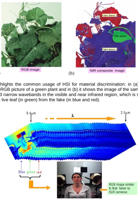
(a) it shows the 3-broad bands of RGB picture of a green plant and in (b) it shows the image of the same plant but using a composite of 3 narrow wavebands in the visible and near infrared region, which is shown capable to discriminate the live leaf (in green) from the fake (in blue and red). ... 18 Figure 2-6 Introduces the concept of hyperspectral imaging (HSI) which is
literally a technique that takes many contiguous narrow waveband images instead of just the 3 broad bands of red, green and blue colours as in the conventional digital photography. ... 18 Figure 2-7. Outlines the components of a typical HSI system which consists of a
spectrograph and a 2D CCD sensor as imaging device. ... 19 Figure 2-8. (a) Shows the schematic ray diagram of the Offner convex
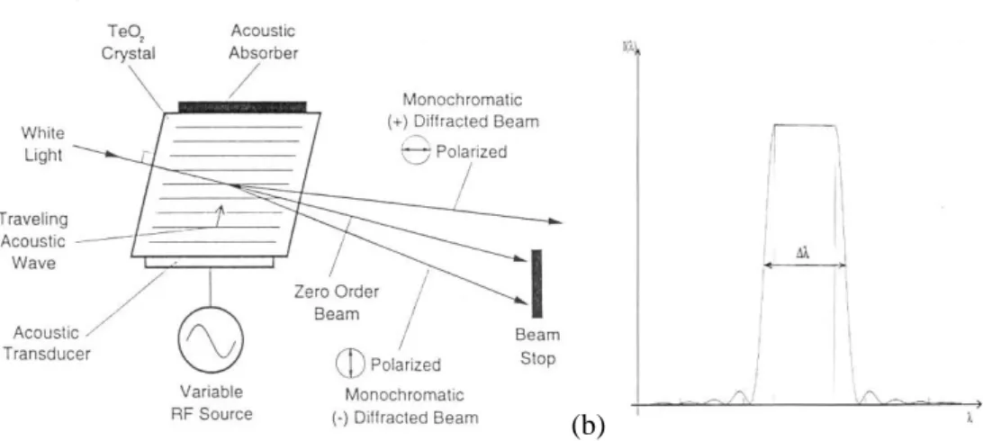
spectrograph. (b) the very compact housing for the Offner spectrograph manufactured by the Headwall Photonics. ... 19 Figure 2-9. Shows the schematic drawing of the PGP based spectrograph ... 20 Figure 2-10. In (a) it shows the schematic working principle of AOTF for MSI
illustrated by using the TeO2 as the piezoelectric crystal and operated in a
non-collinear configuration. One important characteristics of the AOTF MSI is the flexibility of tuning, which not only allowing the user randomly select the pass wavelengths in any spectral order, but also that it enables a variable band width of the passband as shown in (b), and all these features are not possible to be achieved by using the dispersive spectrograph system. ... 21 Figure 3-1 (a) the VNIR HSI camera constructed by our group at DA-CDS which
consists of the Headwall‘s spectrograph and a PCO camera, together with a home built mirror scanner assembly situated at the top of the spectrograph. (b) The two line scanning hyperspectral cameras made by our group and on the left is the PGP based SWIR camera and on the right
is the Offner VNIR system, the red rectangles depict the physical dimensions of the two spectrographs showing how compactness is the Offner design compare with the PGP one. ... 23 Figure 3-2. (a) Shows the AOTF system put together by our group for imaging
in the VNIR spectral range using TeO2 as the active crystal The figure
shows the associate steering optics together with the AOTF spectrograph (in red) which is made by the Gooch & Housego Photonics with transmission characteristics of ~35%, and therefore a high end EMCCD camera (Andor Ixon 897) with a peaked QE of ~90% is employed. Due to the small FOV (~4 ) a 50mm objective lens is deployed as shown in (b). The unit is powered via a separate driver box through standard BNC interface (c). ... 24 Figure 3-3 (a) Outlines the construction of the step motor assembly of the mirror
scanner. (b) A schematic view of the motor housing and the optical axis of the spectrograph and the rotating axis of the step motor. ... 25 Figure 3-4 shows the equipment that has been employed in this study: (from left
to right) the LWIR FLIR SC640, the home built SWIR HSI using a PGP spectrograph, the VNIR AOTF MSI using Gooch & Housego‘s TeO2 AOTF unit, the home built VNIR HSI camera which utilises the Offner spectrograph, and the MWIR SC7600 FLIR thermal imager. ... 26 Figure 3-5. (Left): shows the layout of the experimental setup for the anxiety
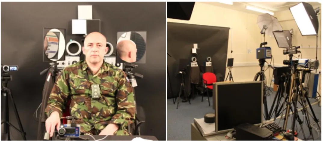
assessment exhibiting a range of calibration panels and black bodies in the background. The room is well illuminated (~750 lux) by diffused halogen lamps as shown in the picture on the right. ... 28 Figure 3-6. shows the representative pictures of the participants involved in this
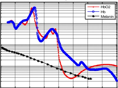
study. Over 2/3 of the participants are from the military background and some participants have repeated the test several times in attempt to study the effects of diurnal variations and food/drink/smoking effects. Note the large variations of the facial flushness over these participants. ... 29 Figure 3-7 Molar extinction coefficients of melanin, oxy-haemoglobin (HbO2),
and deoxy-haemoglobin (Hb) (Prahl, 1999) chromophore in human tissue. ... 30 Figure 3-8 shows (a) Raw thermal image of subject when he starts to answer
the question. (b) Raw thermal snapshot of subject when he almost finishes the question session. (c) The blood flow rate in subject‘s face as he start to answer the question. (d) Blood flow rate in subject‘s face as he almost finish the question session (Ioannis Pavlidis, 2002). ... 34 Figure 4-1Shows the time delay of hormone secretion upon anxiety (a) ACTH
concentration (b) Total plasma cortisol concentration (c) Salivary free cortisol concentration (Kudielka, C, & Hellhammer, 2004) ... 37
Figure 4-2 shows the use of a combined public speaking and cognitive task which can impose a more effective anxiety to the participants. (Dickerson, 2004) ... 38 Figure 4-3 shows the variations of blood pressure, coronary venous flow, and
oxygen extraction ratio and oxygen consumption of a dog under controlled injections of adrenaline (2ug/kg per min at the arrowed point) in an intravenous infusion experiment (Creates, 1980). ... 39 Figure 4-4(a) MBF is the blood flow of masseter muscle. AD represents
adrenaline infusion. The transient increase of masseter blood flow caused by adrenaline is clear in both in 0.1ug/kg and 1ug/kg dose. The larger dose decreases the blood flow lower than baseline after the initial rise. (Ishii, 2009) ... 40 Figure 4-5: shows the false colour image of a subject before (a) and after (b) a
startle. Note that the temperature at around the periorbital region of the subject which is seen to increase by almost 1C after the startle (Levine, 2002). ... 42 Figure 4-6: Highlights the Texas/Honeywell work which intended to demonstrate
the ‗uniqueness‘ of the anxiety signature found in the periorbital region. Shown in the figure is thermal pictures of a subject after (a) Base line b) walk for 1 minute c) walk for 5 minutes d) run for 5 minutes, Note that there is seemingly no increase of temperatures in the periorbital after physical exercising (Murthy, 2006). ... 42 Figure 4-7 Shows the result of the strooping test performed by the Texas group:
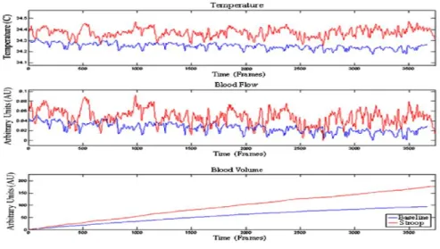
(Top) The forehead temperatures measured by TI technique showing an elevated temperature in the region throughout the test (red) comparing to the base line (blue). (Middle) The ‗interpreted‘ blood flow and (Bottom) the ‗interpreted‘ blood volume calculated by using a computational transfusion model using the temperature as the input. ... 43 Figure 4-8 shows the heat patterns differences of a subject for the activation of
different AU in the face with respected to the base line (Jarlier, 2011) .... 44 Figure 4-9 (a) illustrates the RGB image of a raging monkey. (b) shows the
change of nasal temperature of the monkey (in step of 10s), before and after he was presented a video clip of a raging monkey. White rectangles within the thermal data represent the ROI for temperature measurement. (c) shows the ROI averaged temperature change in response to raging monkey video. It appears apparently that the nose temperature drop down significantly from the baseline after the raging video was presented to the monkey (Akio Nozawa, 2011). ... 44 Figure 4-10.Thermal image of the dorsal side of the right foot during the
stressor experiment ... 45 Figure 4-11. shows the measured blood glucose (MGL) response and the
in a healthy subject on intravenous somatostatin [250 pglhr. SHI: 3 h] (Werner 1992). ... 47 Figure 4-12: shows the long time lag (~30mins) of the blood glucose levels
increase after the stressor is applied. The stressor is applied between 0 to 30 minutes (Wing, 1985). ... 47 Figure 4-13.HBR measurement using TI: Steps 1-3 show the ROI tracking from
the raw TI data. The FFT and the HBR and pulse estimation method are shown in step 4 to 6 (Pavlidis, 2007). ... 49 Figure 4-14Sample thermal images and overlays by the vascular maps in (a)
near and (b) distant poses. The feature labelled by blue point is the ROI for further pulse extraction analysis (Gault, T.R, 2010). ... 49 Figure 4-15.shows the quality of the HBR estimation using CTW technique: (a)
250 frames of raw TI data (b) wavelet coefficients (c). Filtered coefficients, (d) HBR obtained by ICTW (Gault, T.R, 2010). ... 50 Figure 4-16: Shows the physiological based anti-terrorism consortium in the
USA that includes the Texas University, OKSI and the Draper laboratory. We have been contacted by the OKSI for research collaboration in the area of remote sensing of blood oxygenation back in 2011. ... 51 Figure 4-17: Highlights the Lincoln University work for the detection of anxiety
from the face blush and the heart bit rate (HBR). Note that both techniques require the base line information in-prior for the anxiety interpretation. (Yue, 2011). ... 51 Figure 4-18 Outlines some examples of facial Action Units for coding and
identification of facial expression (Ekman, 2002). ... 52 Figure 4-19: Highlights the Bradford University work for the lies detection using
thermal imaging and physical computing of facial expression (Ugail, 2011). ... 52 Figure 4-20: Shows the behaviour detection by trained behaviour detection
officers (BDO) in blue uniforms currently deployed in the USA airports. The methodology is under review due to the extreme in-effective of the approach for anti-terrorism. ... 53 Figure 4-21 Features extracted from multiple ROI for arousal classification: left
supraorbital (LFH), right supraorbital (RFH), left periorbital (LPO), right periorbital (RPO), and nasal (NSP) (Nhan BR,, 2009). ... 54 Figure 4-22: Shows the mobile screening laboratory under the FAST
programme: (a) mobile trailer lab (b) a trial in Maryland consisting of 140 paid volunteers, (c) the acquisition of base line information when participants enters into the trailer (d) participants are monitored by a group of experts who analyse various physiological features during the trial. ... 55
Figure 4-23: Shows the Malintent programme (a) the EO equipment which consists of a thermal camera, a visible camera and a LIDAR. (b) typical thermogram of a participant who is being interrogated (c) typical voice pitch analysis. ... 56 Figure 5-1. Highlight how EO imaging technique detects anxiety from a range of
5 meters. Left panel: Base line, Right panel: after applied emotional stressor. (a) RGB image, (b) StO2 image obtained by HSI, (c) TI false colour images, (d) threshold TI image at 34.4C with black pixel showing temperatures above the threshold. ... 61 Figure 5-2. shows the blood perfusions of a subject when he was in various
emotional states (a) base line, (b) at maximum anxiety, (c) after 2 minutes of anxiety. The perfusion is estimated according to the model illustrated in section 3.3.2. ... 62 Figure 5-3. highlights the physiological response to anxiety through the raising
of HBR when the anxiety begins to set in. Shown in the figure are the HBR of two persons responding to the same stressors (emotional and physical) but the HBR responses from these two persons are seen to be very different. ... 63 Figure 5-4. Shows the heart beat rate detection using thermal imaging (TI)
technique: upper panel- false colour thermalgram of the subject who was sitting in front of the TI with a dumbbell in his hand. Lower panel: the measured HBR (red) and the HBR deduced from the periorbital ROI of the thermalgram (blue) when the subject is exercising the dumbbell. ... 64 Figure 5-5. Shows the heart beat rate detection using MSI technique: upper
panel- false colour MSI image (=600nm) of the subject who was sitting in front of the MSI with a dumbbell in his hand. Lower panel: the measured HBR (red) and the HBR deduced from the face of the subject (blue) when the subject is exercising the dumbbell. This program was developed by AES/ITS and unfortunately it was maliciously removed from our computers by an ex-PhD student who left us at the end of July 2012. ... 65 Figure 5-6. Shows the delay of facial blushing after the peak of the HBR during
the ES session: (a) the thermalgram of 4 subjects when they were at their peak HBR during the ES, (b) the time when they exhibit a maximum flush in their faces. The thermalgrams are in false colours of temperatures, and the pixels exceeding the threshold temperature are presented in black. Note that the threshold temperatures for these subjects are different in each case. ... 66 Figure 5-7. shows the RGB images, the thermalgram and the StO2 of subject A
in the top, middle and bottom panels respectively. a) subject at rest, (b) after ES and (c) after PS. Note the change of temperatures and the StO2 in the forehead, hands and nose during the ES and PS. Both the thermalgram and the StO2 map have been threshold (in black colour) to aid visual observation of the change after the anxiety sets in. ... 67
Figure 5-8. Shows the paling and flushing in the facial region during an ES session: (a)-(d) the thermalgram of the subject taken at a minute interval during the ES session, and note the acute paling in the face after 3 minutes into the ES session. (e-f) Flushing in the face. ... 69 Figure 5-9. Shows one incident of alternative paling and blushing during the ES
session amongst the data that we analysed so far. Shown in the figures are the threshold (Tth=35.45°C) thermalgram of (a) base line of a subject (Caucasian), (b) the moment at the peak of the HBR during the ES, (c) one minute after (b) showing paling in the face, (d) finishes the ES session. .. 70 Figure 5-10. Shows the temperature change in the periorbital region during and
after the ES session: (a) thermalgram of a subject: before (left), during (middle) and after (right) the ES session. The maximum temperature and hot pixels (threshold to 35.4°C) in the periorbital region have been depicted as white and blue colours respectively. (b) the heart beat rate (red), the maximum and mean temperatures in the periorbital region before, during and after the ES session. Note that neither the maximum nor the mean temperature in the periorbital region has increased during and within 2 minutes after the anxiety sets in. Note that this subject is under mild anxiety condition. ... 71 Figure 5-11. Shows the temperature profiles of the periorbital region of the
same subject during and after the ES session: it is cleared from previous figure that the maximum temperature in the ROI has not been increased but the number of hot pixels in the perorbital region, is seen to increase in numbers after a few minutes of the peaked HBR. Note that this subject is under mild anxiety only. ... 72 Figure 5-12 shows the setup of glucose spectroscopic experiment. The sample
is placed directly onto a spectralon which exhibits a flat reflectance of 0.98 over the 300-2500nm wavelength region. ... 73 Figure 5-13 depicts the reflectance spectra of solid samples of glucose, salt and
white sugar that measured in our laboratory using the HSI. ... 74 Figure 5-14 shows the typical water absorption in the visible and swir region (G.
M. Hale, 1973). ... 74 Figure 5-15 shows the reflectance of various concentrations of glucose in water
solution in the SWIR region. The solution is contained in a Perspex box, and note that all the features in the spectra shown are in fact dominated by the water absorption peaks. ... 75 Figure 5-16 Shows the typical reflectance spectra in the SWIR waveband
extracted from various ROI in the facial region of a human subject. The inset shows the false colour image of the subject. The spike point is the noise of the camera. ... 76 Figure 5-17 highlight the spectral difference from the ROI in the face when a
level (base). (a) typical spectra for ROIs in the periorbital and lip regions (b) typical spectra of the forehead and mouth. ... 77 Figure 5-18 shows the differential reflectance between emotional anxiety state
with respected to the base line for (a) periorbital region (b) mouth ROI. Diff(M,B) stands for differential of MS and base line. ... 78 Figure 6-1 outline one of Pavlidis‘s work about the ‗instantaneous‘ increase of
temperature in the Periorbital region when one is under anxiety (Pavlidis et al., 2007). Left: temperature profile of the periorbital region, Right: depicts the location of the ROI in the periorbital region in red. ... 80 Figure 6-2: presents the hot spots in the periorbital region when one is under
anxiety. Shown here are the TI images of 3 subjects (a) subject H, (b) subject P, (c) subject N. Left column: base line, Mid column: when the subject is at the peak HBR during the ES session, Right column: 2-3min rest time after the peaked HBR. All pixels higher than a threshold are labelled in black and the max temperature point is depicted in white. Note that the size of the hot spots has NOT been increased during ES. ... 81 Figure 6-3: shows the number of hot pixels above the threshold in the periorbital
ROI for (a)subject H, (b)subject P, (c)subject N. The 3 zones of baseline, under ES and rest are clearly identified. Note that substantial increase of hot pixels counts in the periorbital region happens only a few minutes AFTER the peak of the HBR. ... 82 Figure 6-4 shows the temperature profile (max and mean) of hot pixels in the
periorbital ROI for (a) subject H, (b)subject P, (c)subject N. Note that temperature in the periorbital hardly increase during the 5 minutes ES session. ... 84 Figure 6-5: shows the hot pixel counts for each temperature zones in the
periorbital ROI for (a) subject H, (b)subject P, (c)subject N throughout the ES session. Note that in most cases it is the pixels in the lower temperature zones that are increasing in number after 2-3 minutes of anxiety. ... 86 Figure 6-6: shows the false colour TI images of the periorbital ROI of subject H
during the ES session ((a)-(h)). The TI image is overlaid by the hot pixels which are colour coded according to their temperature zones. The hot spots evolve like a growing pyramid with the highest temperature in the centre after the anxiety sets in. ... 87 Figure 6-7: shows the mean temperature of the hot pixels in the periorbital ROI
for subject H during a prolonged ES session. It is seen that the mean temperature of the hot spot begins to increase in about 2 minutes AFTER the peaked HBR occurs. ... 88 Figure 6-8: shows the number of the hot pixels in the periorbital ROI for subject
H during a prolonged ES session. Note that the amount of increase in pixels is about 10 times of the base line! ... 89
Figure 6-9: shows the hot pixel counts for each temperature zones in the periorbital ROI for subject H in the prolonged ES session. Similar to the previous results it is noted that the lower temperature pixels are increasing in number after 2-3 minutes of anxiety. ... 90 Figure 6-10: shows the long time lag (~60mins) of the blood glucose levels
increase after the stressor is applied. The stressor is applied between 0 to 30 minutes (Wing, 1985). The surplus glucose can change many physiological responses in the body which can be very misleading as far as remote sensing of emotion as concern. ... 91 Figure 6-11: shows the mean temperature of the hot pixels in the periorbital ROI
for (a) subject H, (b)subject P, (c)subject N during the PS session. Note that there is a long rest time of ~10minutes in (c)... 93 Figure 6-12: shows the number of the hot pixels in the periorbital ROI for (a)
subject H, (b)subject P, (c)subject N throughout the PS session. ... 94 Figure 7-1. Shows the representative MWIR thermalgram of four different
ethnical origins of participants before (left hand panel) and during the MS session (right hand panel). The thermalgram is in false colours representing the temperature, and the black pixels are those above the threshold temperature, which are NOT constant. (a) Male Caucasian b) Female Caucasian c) S American male d) Far-East Asian. ... 96 Figure 7-2. highlights the similarities between the TI and HSI techniques for
anxiety assessment. Upper panel: base line, Lower panel: under anxiety. (a) RGB image of a subject, (b) the false colour StO2 map in scale of [30 60]%, (c) the thresholded StO2 map at 55% of StO2 and the high StO2 pixels are presented in black colour, (d) the threshold thermalgram at 34.34C and the hot pixels are presented in black. While both techniques are found capable to detect the change of blood flow that triggers by anxiety, the HSI seems to be more sensitive in detecting StO2 particularly at around the strategic ROI in the mid forehead (red circle in (c)). ... 98 Figure 7-3. Outlines the variations of skin temperature and oxygenation in one‘s
normal daily routines (a) thermalgram before coffee in the morning, (b) before food, (c) after food, (d) after food and had a cigarette outside. (e)-(h) are the StO2 maps thresholded at 54% (black pixels) corresponding to the thermalgrams presented in (a)-(d). Note the large fluctuation of the skin temperatures in the face and hand even when one is performing normal work in everyday‘s routine activity. ... 99 Figure 7-4. presents the base line images of 14 representative participants in
two columns and each contains the RGB on the right, the false colour StO2 map presented in a fixed scale of [30-55]% in the middle and the thermalgram in the scale of [20 -37.5C] on the left. Note the wide range of the skin temperatures and StO2 variations in their foreheads across these 14 participants. ... 101
Figure 7-5 showing how straight forward it is for assessing one‘s emotional state when the base line information is given. The figure shows the false colour thermalgram of a subject (a) at rest and (b) after ES. The hand temperature is seen to reduce by as much as 3C (~9%) indicating that the subject is in anxiety unambiguously. ... 102 Figure 7-6 shows the forehead and thumb temperatures of 20 participants when
they are in their base lines and under anxiety. Note the large variation of the thumb temperatures across this small sample size of participants. ... 103 Figure 7-7 shows the behaviour of the forehead temperatures upon the trigger
of anxiety: (a) subject B, (b) subject L and (c) subject N. The forehead temperatures are seen relatively stable with changes less than 0.5°C throughout the ES session. ... 104 Figure7-8 shows the behaviour of the nose temperatures upon the trigger of
anxiety: (a) subject B, (b) subject L and (c) subject N. The nose temperatures are seen very responsive to the HBR. Unlike in the forehead it shows very small residual memory effect. ... 105 Figure 7-9 shows the behaviour of the mouth temperatures upon the trigger of
anxiety: (a) subject B, (b) subject L and (c) subject N. The mouth temperatures are seen not as responsive as that of the nose to the HBR, and about ~6% reduction in the mouth‘s temperature due to anxiety has been observed. ... 107 Figure 7-10 shows TI of three participants in four columns of: i) when they are
in their baseline ii) during ES and at their peaked HBR, iii) after 2 minutes of the peaked HBR, and iv) after 5 minutes of the peaked HBR. ... 108 Figure 7-11. highlights the spread of the base line (at t=0) temperatures in (a)
the nose and (b) mouth regions for a selection of subjects. This data implies the need of a reference point in order to relate the change of these temperatures to the degree of anxiety. ... 111 Figure 7-12. highlights the more stable of the temperatures in (a) the forehead
and (b) eye regions for a selection of subjects during the ES session. Note that the base line temperatures of (a) & (b) are found closely correlated. 112 Figure 7-13. shows the ill-defined relationship between the physiological
properties such as the change of the HBR with respected to the amount of the cortisol in the saliva for four participants who experience various degrees of anxiety during the ES session. ... 114 Figure 7-14. By using labelled data sets one can deduce the relationship
between the EO quantities with respected to the level of anxiety. The figure plots the DFNSO & DFMT obtained from highly stressed subjects (see Table 7-6) together with those of the base line (see Table 7-7), and it results in a very well-defined two clusters representing two regimes of high and low anxiety. The boundary at the DFNSO of 2.75 which corresponds to
the DFMT of 1.8 may then be used for anxiety classification into high and
low categories. ... 116
Figure 7-15. Showing how the DFMT can be correlated to physiological properties such as the heart beat rate. The figure presents the DFMT and the HBR of one subjects during the ES session, and it is seen that the DFMT follows the HBR with a small time lag as mentioned in previous sections. ... 119
Figure 8-1 outline the functionality of right and left brain according to Sperry‘s theory. (Sperry, 1980) ... 121
Figure 8-2 (Left) Shows the false colour TI image of a subject and the assignment of the ROI on his forehead. (right) typical skin temperatures of the 4 ROIs while they are performing different natures of tasks. ... 124
Figure 8-3 shows the differential temperatures between the left (ROI 4) and the right (ROI 1) for a number of subjects after they performed 4 different kinds of tasks. Note that the temperature difference seems to be very small for the recognition task. ... 124
Figure 8-4 plots the differential temperatures between ROI1 and ROI4 against the HBR. The data due to the recognition/memory task seems to be well clustered (in black) with clear boundary well separated from the mental maths task (in red). ... 125
Figure 10-1: shows the set up menu of the HSI control software designed and developed by the author: (a) VNIR HSI camera. (b) SWIR HSI. ... 129
Figure 10-2:shows the setup menu for the control of the AOTF MSI system that has been developed by the author. ... 130
Figure 10-3:Shows the typical ‗composite‘ images collected by the three spectral cameras (a) VNIR HSI (b) SWIR HSI (C) AOTF MSI using the acquisition software established by the author. ... 130
Figure 10-4: gives the SDK layout of VNIR and SWIR ... 131
Figure 10-5: highlights the flow chart of MSI SDK ... 131
Figure 10-6highlights the flow chart of VNIR and SWIR ... 132
Figure 10-7: exhibits the possible states of thread that operating system may give ... 134
Figure 10-8: shows the single thread software procedure ... 134
Figure 10-9: gives the flowchart of multi-threading configuration of MSI imaging system ... 135
Figure 10-10 Shows the sample thermal image of participant and the experimental setup of angle measurement. ... 136
Figure 10-11: Shows the sample thermal image of black body and the experimental setup for the black body temp measurement. ... 137 Figure 10-12: Shows the least-squares regression line for blackbody and
human forehead temperature (Mwave) and the value of cosine angle.The blue star illustrates the real temperature value against the cosine value of angle. ... 138 Figure 10-13: illustrates the least-squares regression line for blackbody and
human forehead temperature change percentage (Mwave) and the value of cosine angle. The blue star shows the real temperature change percentage value against the cosine value of angle. ... 139 Figure 10-14: Shows the least-squares regression line for blackbody and
human forehead temperature (Lwave) and the value of cosine angle. The blue star illustrates the real temperature value against the cosine value of angle. ... 140 Figure 10-15: illustrates the least-squares regression line for blackbody and
human forehead temperature change percentage (Lwave) and the value of cosine angle. The blue star shows the real temperature change percentage value against the cosine value of angle. ... 140 Figure 10-16shows an example of the black body temperature measured by a
cooled MwaveTI camera (NETD ~20mK and LWIR uncooled TI camera (NETD~35mK). The blackbody temperature is set from 26 to 45 degree, shown in the x axis. The y axis gives the corresponding temperatures Measured by the two TIs. ... 142 Figure 10-17Shows the hot pixel number of periorbtial region of the subject H
measured by LWIR uncooled TI camera (NETD~35mK). ... 142 Figure 10-18Shows the nose Mean temperature of the subject N Measured by
LIST OF TABLES
Table 4-1 Shows the classification accuracies for the arousal states: high arousal(HA) versus base line(BASE), low arousal (LA) versus BASE, HA versus LA (Nhan BR,, 2009). ... 54 Table 6-1: A summary of the temperature in the periorbital region after the ES
session. ... 95 Table 7-1: Highlights how sensitive is the temperature of finger/hand to dietary and
weather conditions other than that triggered by anxiety. Noted the very large standard deviation in these figures... 100 Table 7-2: shows the variation of nose and mouth temperatures due to other
environmental factors. Noted the very large standard deviation in these figures. ... 100 Table 7-3 tabulates the variations of the HBR and the mean nose temperatures for a
number of participant during ES session. ... 109 Table 7-4 tabulates the variations of the HBR and the mean lip temperatures for a
number of participant during ES session. ... 109 Table 7-5 tabulates the change of the HBR, the mean nose and lip temperatures for
a number of participant between the baseline and when they are under anxiety. ... 110 Table 7-6 Anxiety assessment data for 4 selected subjects. ... 114 Table 7-7 Presents the base line data of several subjects and they are analysed by
using the DFMT and the DFNSO method as a test bed. Scores of below 1.8 and 2.75 for the DFMT and DFNSO respectively imply the absence of anxiety. Yellow colour: Civilians subjects, green: military subjects, orange: high blood pressure subject, red: alcoholic test, pink: false alarm. ... 115 Table 7-8 Shows the anxiety assessment results without the base line information
using the classification method that has been developed in this project. The anxiety is classified as high when the DFNSO and DFMT values are over 2.75 and 1.8 respectively; otherwise the anxiety status is classified as low or no anxiety. The result is colour coded, and the ground truth is based on the cortisol level together with a consultation with the subject. Green=positive positive, Yellow=negative negative, Pink=positive negative, red=negative positive, purple=high cortisol above 0.17mg/mL ... 118
LIST OF EQUATIONS
'/
W W
Equation 2-1 ... 10 0 4 0 0( )
1
( )
W d
W d
T
W d
Equation 2-2 ... 11 1 Equation 2-3 ... 11 Equation 2-4 ... 11 '/ W
W Equation 2-5 ... 11 4*
j
T
Equation 2-6 ... 11 4 4 / T T
Equation 2-7 ... 11 (1 ) Equation 2-8 ... 12 maxb
T
Equation 2-9 ... 12 E hv Equation 2-10 ... 13 3 22
1
( , )
1
hv kThv
I v T
c
e
Equation 2-11 ... 13 B( Equation 2-12 ... 13 Equation 2-13 ... 13 Equation 2-14 ... 15 Equation 2-15 ... 15 Equation 2-16 ... 15 Equation 2-17 ... 16 Equation 2-18 ... 22l
lc
A
Equation 3-1 ... 31 effHb Hb effHbO HbOC
C
A
2 2
Equation 3-2 ... 31 effmelanin melanin effHb Hb effHbO HbOC
C
C
A
2 2
Equation 3-3 ... 31G
DPF
lc
A
Equation 3-4 ... 32G
C
A
eff
Equation 3-5 ... 32G
C
C
A
HbO2 effHbO2
Hb effHb
Equation 3-6 ... 32
G
C
C
C
A
HbO2 effHbO2
Hb effHb
melanin effmelanin
Equation 3-7 ... 33
Qr Qe Qf Qc Qm Qb Equation 3-8 ... 34
Equation 3-9 ... 34
LIST OF ABBREVIATIONS
AOTF Acousto-optical tuneable filters A/D Analog-to-digital
AU Action unit
bpm Beats per minute
BDO Behaviour detection officers BL Beer-Lambert Law
CRH Corticotropin-releasing hormone CTW Continuous wavelet transform COTS Commercial-Off-The-Shelf
CO2 carbon dioxide
CU Cranfield University
DFMT Differential Forehead Mouth Temperature DFNSO Differential Forehead Nose StO2
EO Electrical optical ES Emotional anxiety
EA Emotional Anxiety
EBL Extended Beer-Lambert Law ELM Empirical Line Method
fMRI Functional Magnetic Resonance Imaging FPA Focal plane array
FOV Field of view
FMRI Functional magnetic resonance imaging FFT Fast Fourier Transform
FACS Facial Action Coding System fps Frames per second
Hb Deoxy-Haemoglobin
HbO2 Oxy-haemoglobin
HSI Hyperspectral Imaging
HPLC High performance liquid chromatography Hb Deoxy-haemoglobin
HbO2 Oxy-haemoglobin
HPA Hypothalamic–pituitary–adrenal HBR Heart beat rate
HSI Hyperspectral imaging
IED Improvised explosive devices ICWT Continuous wavelet transform LBF Limb blood flow
LCTF Liquid crystal tuneable filters LWIR Long wave infrared wavelengths MOD Ministry of Defence
MSE Mental strong emotions
MWIR Mid wave infrared wavelengths MGL Measured glucose level
MHC Metabolic heat conformation MSI Multispectral imaging
NEDT Noise equivalent differential temperature
NIR Near Infra-Red
PA Physical Anxiety
PO2 Partial pressure of Oxygen
ROI Region of Interest PS Physical anxiety PGP Prism-Grating-Prism PSE Physical strong emotions ROI Region of interest
SDK Software Development Kit SiTF Signal transfer function SH Stand horse
SDK Software Development Kit StO2 Tissue Oxygen Saturation SWIR Short Wave Infra-Red TI Thermal imaging
TSST Triers Social Anxiety Test
TI Thermal Imaging
VIS Visible
VNIR Visible Near Infra-Red
2D Two-Dimensional
1 Introduction
1.1 Objective of Research
This PhD project formulates part of the research programme towards the understanding of how human‘s physiological features can be captured from stand-off distances. This is a basic research and the ultimate objective of the overall research programme is to understand how these remotely acquired physiological features can be deployed for assessing one‘s emotions. In this study two main kinds of basic emotions have been considered: (1) Clam emotion and (2) Strong emotions specifically anxiety due to (a) panic and anxiety resulting from psychological pressure and (b) pain or fatigue resulting from physical demands. These two different kinds of emotions in (a) and (b) are denoted as mental (MSE) and physical strong emotions (PSE) in this thesis.
This PhD project focuses on the remote sensing of physiological features in the facial region, together with heart beat rate (HBR) and a first attempt of glucose level assessment using Electro-Optical (EO) imaging technique. The research involves three main parts: (a) instrumentation design and experimental set up, (b) properties of physiological features in the facial region acquired by remote sensing technique and (c) how these physiological features can be used for the detection of strong emotions, such as anxiety, due to emotional or physical stimulations or stressors. The project was initially funded by the UK MOD and the Directed Research programme, and it was later partially supported by the InnovTech Solutions (ITS) Ltd particularly in the area of heart beat rate (HBR) detection development. Subsequently all publication related to this work needs the consents from both UK MOD and ITS.
1.2 Motive of Research
The research for the detection of human‘s emotional states from standoff distances without direct contact with the object, have been one of the greatest demands in biomedical, man-machine interfacing, and affective computing sectors. Conventional methods have largely been using facial expressions (Edwards, Jackson, & Pattison, 2002)(Fasel & Luettin, 2003) for the remote sensing of people‘s emotional state,
however, the facial expressions can be suppressed by will, which makes this approach not robust enough for the detection of malicious intent. Involuntary physiological responses under the command of the sympathetic nervous system such as body sweat, heart rate, breath rate, body temperature, blood perfusion and oxygenations, have been proposed (Chen, et al., 2009)(Yuen P. , et al., 2009) as a tool to monitor the emotional states of people (Pavlidis, Levine, & Baukol, 2001)(Pavlidis & Levin, 2002).
One novelty in this work is the use of EO imaging technique for the detection, and subsequently classification, of human‘s emotional state from a stand-off distance for the very first time (Yuen P, 2009). The basis of the present work is based on the fact that elevated level of adrenaline is secreted into the blood stream when a person is experiencing extreme emotional or physical conditions causing anxiety or excitement, which in turn triggers an elevated heart beat and breathing rates resulting in an increased level of blood perfusion and StO2 in the body. This work serves as the first study in the field thus to allow other researchers in the community to continue the approach for a deeper understanding of how physiological features can be used for the classification of human‘s emotional states.
1.3 Contribution and Achievements
One innovation in this study has been using multiple physiological features extracted from thermal and hyperspectral imaging (HSI) technologies to assess people‘s emotional state semi-quantitatively from a stand-off distance for the very first time. The detection includes the remote sensing of HBR and the assessment of blood transfusion in the forehead region.
The main contributions of this research have been:
i) To produce new evidences to invalidate the deeply believed concept of an increased skin temperature in the perorbital region when strong emotional states such as anxiety is taking place.
ii) The development of capability for the remote sensing of heart beat rate (HBR), facial physiological features and glucose level using imaging technique.
iii) The first attempt for using electrical optical (EO) technology for the remote sensing and classification of human‘s emotional state without the need of base line information.
1.4 Thesis layout
The layout of this thesis is arranged in the following manner: the motives and the objectives of the project are highlighted in chapter 1, which is then followed by a review of EO imaging techniques in chapter 2. The experimental set up and the methods for the data analysis employed in this work are described in chapter 3. This chapter includes a review of the principles and theories of thermal emission, diffuse scattering, Beer-Lambert law for the StO2 assessment and blood perfusion models adopted in this work. Subsequently a survey of remote sensing of emotions is given in chapter 4, followed by a description of the EO signatures found in this work in chapters 5. Chapter 6 outlines the main results for the clarification of the anomaly temperature induced by anxiety in the periorbital region, and chapter 7 describes the main technique developed in this study for the remote assessment of emotions without base line information. Chapter 8 address the issue for using EO data for emotion classification and finally the main conclusion of this work is summarised in chapter 9.
2 Introductions of Electro-Optical imaging techniques
When an object is illuminated by light it is quite common that not all the incident energy is absorbed: part of it will be transmitted, and part will be reflected and some of the absorbed energy will be re-radiated. The electromagnetic band in the visible to near infrared (VNIR) ranging from 400nm-2500nm wavelength region is commonly termed as the reflective band, as most of energies in this waveband is scattered back into the space from the illuminated object. Longer wavelengths beyond 3m are known as radiative or emissive band due to the fact that they are the photon energies that are re-radiated from the body of the illuminated objects.
In this study we have utilised sensors in both the reflective and emissive bands to capture the physiological features of people with a view to understand their emotional states without direct contact with them. These two classes of sensors and their operation principles are briefly outline in the next two sections.
2.1 Sensing of emissive band by thermal imaging (TI)
Thermal imaging (TI) senses predominantly the emission bands in the mid and long wave infrared (MWIR/LWIR) wavelengths to deduce the ‗temperature‘ of the emissive body. The amount of radiation emitted from various parts of an object keeps in pace with the temperature change across the surface of the object, thereby the thermal image presents an outlook of temperature variations over the object. With the advent of highly sensitive thermal camera off the shelf, temperature measurements can be made remotely during the day and at night. Thus TI has been deployed widely including geological mapping and military applications.
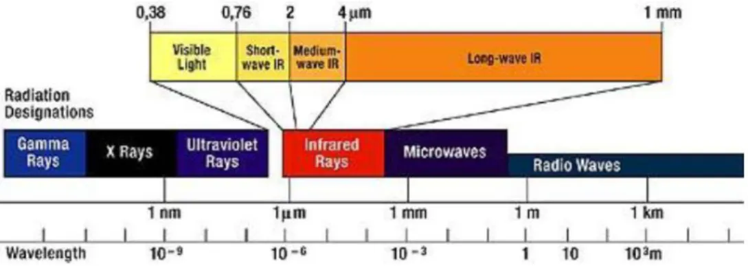
Bounded by the visible and the microwave spectral bands, the infrared light spans 3 orders of magnitude in wavelengths and it is normally divided into (a) the near infrared spans from 0.7 to 3 μm, (b) the middle wavelength infrared band 3-14 μm, and (c) the far infrared spans from 14 to 1000 μm, respectively. The near infrared is being used for telecommunications and remote sensing, e.g., to study land using and geological mapping. Long wavelength and middle wavelength infrared find its main use in thermal imaging. The wavelength range of interest in the present study has been the VNIR, MWIR and LWIR regions (figure 2-1).
Figure 2-1 Wavelength of interest of the electromagnetic spectrum in the present study: VNIR and LWIR.
2.1.1 Overview of radiative theories
Emissivity is a term describing a material‘s ability to emit thermal radiation and it varies considerably from substance to substance spanning anything from zero to one. It is noted that the black body has been a theoretical object which does not exist in real life and thus the extent of radiations from all objects are in fact less than their true temperatures. Further complication of the issue is that radiative emission is a property not only stemming from the material‘s temperature characteristic, but also that it depends on the spectral wavelength, as well as the angular emission angle which is hardly isotropic. In most engineering applications it is however assumed that the surface‘s spectral emissivity behaves like a constant and in this case it is commonly termed as the grey body assumption.
Since many substances are capable to reflect or transmit a part of the incident radiation, the radiation energy that is absorbed and emitted will be less than that of blackbody. Non-blackbody emitter can only emit a fraction of radiation energy with respect to the blackbody at the same temperature. Therefore, the emissivity can also be defined as a measurement of the maximum amount of radiation that a substance is able to emit.
2.1.1.1 Emissivity and Kirchhoff’s Law
The emissivity is defined as ratio of the radiant emittanceW' of the source to the radiant emittance of a blackbody W at the same temperature:
Emissivity is a function that dependent on the wavelength and the temperature of the material. A more general expression in terms of the spectral emissivity ( ) is
0 4 0 0
( )
1
( )
W d
W d
T
W d
Equation 2-2 Where Wλ is the spectral emitted radiation, ε denotes the emissivity and T is theabsolute temperature, σ is the stefan‘s constant. Note that the emissivity ( ) can be =1, or = constant, or varies with wavelength.
Thermal radiation over a body is usually categorized into three portions: transmission, absorption, and reflection. When a given radiant energy is incident on a surface there are three situations that may happen: a fraction of the incident energy α may be absorbed by surface, a fraction p may be reflected to air and a fraction Γ may be transmitted through substance. Due to the fact that energy must be conserved, the sum of these terms must be equal to one:
1 Equation 2-3 The absorptivity is the ratio of the energy absorbed by the object to the incident energy for a particular wavelength. The absorbed energy will be proportional
to where is the intensity of black body radiation at wavelength
and temperature T. The emissivity of the object is where is the emissivity at wavelength . For a black body this yields:
Equation 2-4 W'/
W Equation 2-5 This is also commonly known as ―good absorbers are good emitters‖ and the Stefan–Boltzmann law describes the total energy radiated from per unit surface area of a black body in unit time ( j*) which has been shown to be proportional to the fourth power of the black body's absolute temperature T:
4
*
j
T
Equation 2-6 To combine the Kirchhoff‘s law with the Stefan-Boltzmann‘s law:
From this it follows that = . Thus the emissivity of any material at a given temperature is numerically equal to its absorptions at that temperature. For an opaque material it does not transmit energy and thus ( ) = 1 and:
(1 ) Equation 2-8 2.1.1.2 Wien's law
The temperature-dependent spectrum of radiation emitted by a black body is termed as black-body radiation and at room temperature it emits nearly all wavelengths which are mostly in the infrared. The peak of the blackbody radiation tends to move towards longer wavelengths with lower intensities when the temperature reduces (see figure 2-2). The Wien's displacement law has shown that the spectral distributions of blackbody radiation at different temperatures are in a trend according to an inverse relationship between the black body temperature and its peak wavelength of emission: max
b
T
Equation 2-9Where λ max is the peak wavelength in meters, T is the temperature of the blackbody in Kelvin‘s (K), and b, normally refers to Wien's displacement constant.
Figure 2-2 shows the Wien‘s law of black body radiations which exhibits a characteristic peak of radiation intensity moving towards to shorter wavelengths as the temperature of the black body increases.
It is noticed that both the Wien‘s and the Rayleigh-Jeans law has got problems which seem to work well only in the short and long wavelengths respectively. Subsequently Planck proposed a radiation function based on quantum mechanical principle:
E hv Equation 2-10 3 2
2
1
( , )
1
hv kThv
I v T
c
e
Equation 2-11where is spectral radiance, or energy per unit time per unit surface area per unit solid angle per unit frequency or wavelength (as specified), is frequency, is temperature of the black body, is Planck constant, is speed of light, is Boltzmann constant. Planck function is only practically valid only when many photons are being measured.
2.1.1.3 Angular dependence of emissivity
Real objects are not perfect emitters and will therefore emit less radiance than a blackbody. The spectral emissivity , is a measure of the effectiveness of an object as a radiator. For Lambertian surfaces, the emitted radiance is distributed equally into the hemisphere above the surface. The self-emission for Lambertian surfaces is defined as
B
(
Equation 2-12 Most materials are not Lambertian and the emissivity term is modified to incorporate this dependence on viewing angle. The self-emission for non-Lambertian surfaces is then
Equation 2-13 Where ( ) indicate the direction of the sensor. The parameter is known as the directional emissivity.
The emissivity of a material is a function of the angular emission, wavelength and temperature. For example the emissivity of water varies considerably from band to band, and at wavelength of 10 um it is a perfect blackbody while it becomes a mirror at ‗low‘ angle of emission (ie ~90). Shown in figure 2-3 is the emissivity value simulated for human skin using a dielectric model (Shahram, 1992) at the wavelength of 10um using polarised (E & O) and unpolarised light as functions of
angle of emission. It is seen that the emissivity spans from zero to one for the emission angles of 0 to 90 degree with respected to the normal of the plane.
Figure 2-3 shows the angular dependence of emissivity in human skin simulated for 10um wavelength and note that the emissivity stays constant for the emission angles less than 60 degree with respected to the normal of the plane (Shahram, 1992).
2.1.2 Infrared Detects
There are two main different types of infrared detectors, namely the photon and thermal detectors.
2.1.2.1 Photon Detectors
Photon detectors directly convert incoming photons into photocurrents. In a photodiode, incoming photons are absorbed and generate electron-hole pairs that are given rise to a photocurrent. For the photons to be absorbed by the semiconductor, the band gap of the semiconductor must be higher than the photons‘ energy. For a given material, the achievable photodiode signal-to-noise ratio depends on the ratio α/G, where α is the absorption coefficient and G the rate of thermal generation of free charge carriers. In the LWIR range, i.e., the most suitable range for thermal imaging, it is required to cool down the semiconductor to cryogenic temperatures (≤ 77K) in order to obtain a good performance.
2.1.3 Thermal Detectors
Thermal detectors are one kind of photon detectors in which it firstly convert photons into heat before measuring the induced change in temperature. There are several physical mechanisms that can be used to measure this change in temperature.
2.1.3.1 Pyroelectric Detectors
Pyroelectric detectors use pyroelectric materials to measure the temperature change caused by infrared radiation. Pyroelectric materials are materials that change polarization upon change in temperature. Pyroelectric detectors can only operate in AC mode, as free charges will cancel the obtained polarization in DC. The current flowing into or out of a pyroelectric detector is made out of two electrode in between which is a pyroelectric material and the current is given by
Equation 2-14
Where A is the area of the electrodes, p the pyroelectric coefficient, and dT/dt the rate of temperature change.
2.1.3.2 Thermo-mechanical Detectors
Thermo-mechanical infrared detectors use deflection of composite cantilevers made of two materials having different coefficients of thermal expansion. The deflection at the tip of the cantilever is given by
Equation 2-15 Where C is a constant that depends on the materials‘ thicknesses and their Young‘s modulus, L is the length of the cantilever, and α1 and α2 are the coefficients of thermal expansion of the two layers. There are several ways this deflection can in turn be measured, e.g., optical reading (deflection of a light beam on the cantilever), capacitive sensing ,or piezoresistive sensing.
2.1.3.3 Bolometers
Bolometers are thermal sensors that use a thermistor to measure the temperature change induced by incident infrared radiation. The change in bolometer resistance due a change in temperature is given by
Equation 2-16 Where α is the temperature coefficient of resistance of the thermistor and the temperature change due to the incident radiation.
2.1.4 Thermal Camera
A thermal camera is a non-invasive device that detects IR energy and converts it to an electronic signal, which is then processed to produce a thermal image. Therefore, radiation energy from the object as sensed by camera can be accurately quantified. In order to operate thermal camera effectively without being affected by the noise arising from the dark current, most TI cameras normally employ a number of detector elements together with cooling system. There are also uncooled FPA-type (focal plane array) cameras which is more affordable but with a trade-off of having lower sensitivity.
In the areas of imaging system analysis, image quality specification and sensor trade-off studies are most commonly refer to spatial resolution and sensitivity. The sensitivity is normally defined as the noise equivalent parameter that would lead to the radiance difference of the target with respected to that of the background.
A thermal camera can be characterised by its signal transfer function, noise equivalent temperature difference, contrast transfer function and minimum resolvable temperature difference. Signal transfer function (SiTF) is the slope of the linear portion of the response function of a system. The responsivity function is defined as the output to input transformation in which the target size is fixed and the target intensity is varied. It is typically S-shaped as shown in Figure 2-4. For many systems, the electronics have a limited dynamic range compared to the detector and the output is therefore designed to centre at about some average value. Saturation in the positive and negative directions about this average value is typically limited electronically by the dynamic range of an amplifier or analog-to-digital (A/D) converter.
Noise is defined in the broadest sense as any unwanted signal components that arise from a variety of sources. The RMS noise voltage can be referred to the input that produces an SNR of unity. The noise equivalent differential temperature (NEDT) is a measure of system sensitivity. The system noise signal can be measured as the output signal when no useful input signal is applied. Once SiTF is obtained from the responsivity function, the NETD can be calculated as follows
Figure 2-4 Typical responsivity function illustrating the SiTF.
2.2 Hyperspectral imaging (HSI)
Hyperspectral imaging (HSI) is a spectral sensing technique which takes hundreds of contiguous narrow waveband images in the visible and infrared regions of the electro-magnetic spectrum (figure 2-2) (Shaw & Burke, 2003) (Smith R, 2006). The image pixels form spectral vectors which represent the spectral characteristic of the objects in the scene and therefore HSI has been mostly applied for material identifications and discriminations purposes. Although HSI was originally developed for mining and geology applications, its usage has quickly spread into other civilian sectors and more recently into the military sector due its capability of material discrimination (Goldberg, 2003). In military and security applications the technique has been specifically adopted for the detection and recognition of targets which are normally well camouflaged with respect to the background and hence HSI is designed as a counter-countermeasure allowing ‗look-alike‘ targets to be differentiated (Yuen, 2006). As illustrated in figure 2-5, which depicts the red/green/blue (RGB) image of an apparent green leafy plant (figure 2-6a) but in fact there is only one live leaf and the rest of them are fake leaves. This highlights the need of a technique like HSI which exploits information in high spectral resolutions
over a wide spectral range to allow the discriminative detection of targets even when they exhibit subtle spectral contrast with respect to the background.
(a) (b)
Figure 2-5. Highlights the common usage of HSI for material discrimination: in (a) it shows the 3-broad bands of RGB picture of a green plant and in (b) it shows the image of the same plant but using a composite of 3 narrow wavebands in the visible and near infrared region, which is shown capable to discriminate the live leaf (in green) from the fake (in blue and red).
Figure 2-6 Introduces the concept of hyperspectral imaging (HSI) which is literally a technique that takes many contiguous narrow waveband images instead of just the 3 broad bands of red, green and blue colours as in the conventional digital photography.
2.2.1 HSI instrumentations: an overview
HSI collects large numbers of contiguous narrow spectral bands for a scene forming a hyperspectral cube (figure 2-6) which contains two dimensions of spatial and one dimension of spectral content (Shaw & Burke, 2003) (Smith, 2006). In the heart of the HSI instrumentation is the spectral dispersion mechanism which is known as spectrograph (figure 2-7), and it exists in various different forms of which the most
RGB image RGB image
Fake leave 1 Fake leave 2
live leave
common three categories have been the dispersive spectrometer, the Fourier transform interferometer and the narrow band tuneable filter. Details of these spectrographs can be found in the literature by Vagni (Vagni, 2007).
Figure 2-7. Outlines the components of a typical HSI system which consists of a spectrograph and a 2D CCD sensor as imaging device.
(a) (b)
Figure 2-8. (a) Shows the schematic ray diagram of the Offner convex spectrograph. (b) the very compact housing for the Offner spectrograph manufactured by the Headwall Photonics.
2.2.2 Dispersive spectrograph
Dispersive imaging spectrometer employs either a grating or prism for light dispersion. The hyperspectral cube is formed by sensing one line of image such that the spatial and spectral information is stored in each dimension of the 2D sensor array. This means that the system can only image a line of the scene at a time and this is commonly realised through a s
the objective lens (see figure 2-8). A prism has advantages of having high efficiency and low scatter, but their optical design tend to be considerably more complex than their grating-based counterparts.
Figure 2-9. Shows the schematic drawing of the PGP based spectrograph
Gratings can be