Implied correlation indices and volatility
forecasting
Holger Fink
a,1, Sabrina Geppert
a,2September 13, 2015
abstract
Implied volatility indices are an important measure for 'market fear' and well-known in academia and practice. Correlation is still payed less attention even though the CBOE started to calculate implied correlation indices for their benchmark S&P500. However the lit-erature especially on cross-country dependen-cies and applications is still quite thin. We are closing this gap by constructing an implied correlation index for the DAX and taking a deeper look at the (intercontinental) relation-ship between equity, volatility and correlation indices. Additionally we show that implied cor-relation can eectively improve volatility fore-casting models.
authors info
aChair of Financial Econometrics, Institute
of Statistics, Ludwig-Maximilians-Universität München, Akademiestr. 1/I, 80799 Munich, Germany
1[email protected] 2[email protected]
keywords
implied correlation, implied volatility, correla-tion indices, volatility indices, volatility fore-casting
JEL subject classification C1, C58, G15, G17
1 Motivation
For foreign exchange options, the concept of implied correlation is well-known and easy to grasp as the fact that two exchange rate multiplied together lead to another one helps to uniquely identify implied correlation by just considering classical vanilla options. Consequentially, several studies are available in this area (e.g. Siegel (1997), Campa and Chang (1998) or Walter and Lopez(2000)) showing among other things a positive dependence structure between volatility and correlation.
However, for equity indices, the situation gets more delicate as one would need reliable options prices of bivariate options on all index components. To overcome this obstacle, the assumption of equal implied correlation for all single stocks ('equicorrelation') is usu-ally made. In 2009, as the rst global exchange, the CBOE began calculating implied correlation indices for the S&P500 (which we will from now on call by its Bloomberg shortcut 'SPX') as a measure for an average expected market dependence. The heuristic of their methodology consists of comparing an estimator for the at-the-money (ATM) implied volatility of the index with a weighted sum built from ATM volatilities of a 50-stock-subindex (cf. Chicago Board Options Exchange(2009)) and is implicitly built on the mentioned equicorrelation assumption.
While several studies like Fleming et al. (1995), Christensen and Prabhala (1998),
Fleming (1998), Blair et al. (2001), Corrado and Miller Jr. (2005) or Fernandes et al.
(2014) already stressed the importance of implied volatility indices like CBOE's VIX, the literature on implied equity correlation is still quite thin. One of the rst authors to actually calculate an equity implied correlation index wasSkintzi and Refenes(2005) who also showed that (similar to volatility) it provides a better forecast for future correlation than using historical data. Furthermore, Driessen et al. (2009) deducted that implied correlation might carry a negative risk premium whileHärdle and Silyakova(2012) have investigated correlation based trading strategies.
and to encourage exchanges and data providers to follow the CBOE and include such indices in their portfolio. In order to do that, we calculate an implied correlation index for the German equity index DAX and investigate the intercontinental dependencies with the SPX and its volatility and correlation indices. Even though, for the sake of comparability, we will mirror the procedure from CBOE, we want to remark thatLinders and Schoutens
(2014) recently pointed out some potential weaknesses of this concept. Furthermore, we will show that the inclusion of implied correlation in a classical ARMAX model leads to an improved forecasting of implied volatility levels.
All computational considerations where carried out in MATLAB using Kevin Shep-pards MFE Toolbox (cf. Sheppard(2013)).
2 Correlation index construction
In order to reach comparability, we will construct DAX-implied correlation indices based on the procedure of the CBOE S&P 500 Implied Correlation Index (called 'CIX' in this study) described in detail byChicago Board Options Exchange(2009). The basic idea is to compare for each dayt≥0, the implied volatilityσIndex,tof an ATM-index option with
the respective implied volatilities σit of (generally) each individual component. Under
the equicorrelation assumption (which was also recently used for volatility correlation by
Aboura and Chevallier (2014)), we can derive the (average) implied correlation of the index and dene
Implied Correlation Indext=100⋅
σ2 Index,t− ∑ N i=1w 2 itσit2 2∑N−1 i=1 ∑ N j>1witwjtσitσjt (1) where(wit)i=1,...N are the components' index weights given by
wit=
Sit⋅Xit
∑N
i=1Sit⋅Xit
with (Sit)i=1,...N being the respective share prices and(Xit)i=1,...N the number of
free-oating shares.
To obtain approximations of the ATM-volatilities, we chose on each trading day for all components the closest put at or below the underlying and the closest call at or above the underlying and linearly interpolate between both. For the index itself, a similar procedure based on the forward price calculated via the put-call-parity is used (cf. Chicago Board Options Exchange(2009) for details). Since the DAX is a total return index, its volatilities were calculated viaBlack and Scholes(1973) while for the typical American single stock options the method of Barone-Adesi and Whaley(1986,1987) was applied.
We interpolated the riskless term structure by taking EONIA, 3m-, 6m-, 9m- and 12m-EURIBOR in addition to the return of the 2-year REX representing syntectic prices for German government bonds - this procedure is similar to the calculation of the VDAX-NEW (cf. Deutsche Börse(2007)).
Our chosen time frame starts after the triple witching day 20. December 2010 and goes until 16. November 2012, the expiration day of the respective CIX 2012. To be inline with
Chicago Board Options Exchange(2009), we therefore need to calculate three correlation indices using options maturing end of 2011, 2012 and 2013 (cf. Table 1). Respective
Correlation indices Time period CDAX 2011 20.12.2010 12.12.2011 CDAX 2012 01.12.2011 16.11.2012 CDAX 2013 01.12.2011 16.11.2012
Table 1: DAX correlation indices
option maturities were 16. December 2011, 15. December 2012 and 20. December 2013. The indices themselves have a lifespan of 2 years. As a consequence, for each trading day, 2 correlation indices are available (inline with the CIX).
All used (underlying/option) closing prices, free-oating market cap, dividend esti-mates and rates were taken from Thomson Datastream. Due to incomplete option data for Commerzbank AG, Fresenius SE & Co. KGaA, Merck KGaA and MAN SE these underlyings were excluded from the correlation indices. In contrast to the CIX which
are only based on the 50 top components in terms of market cap, the CDAX indices are principally built on the whole DAX. We want to remark that on 24. September 2012 MAN SE and Metro Group were excluded from the index and exchanged for Continental AG and Lanxess AG. To avoid a potential bias by increasing the considered single stocks, we interchanged Metro Group with Continental AG and left Lanxess AG out. In terms of time horizon and number of stocks, our data setup is therefore similar to Härdle and Silyakova(2012).
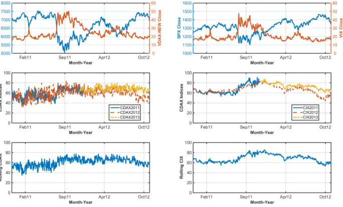
Figure 1: Top: DAX, VDAX-NEW, SPX and VIX closing prices. Middle: CDAX and CIX indices. Bottom: Rolling CDAX and CIX indices.
The new CDAX indices, the VDAX-NEW (for ease of notation from now on just called 'VDAX'), the DAX and their respective US counterparts are depicted in Figure 1. The
later ones are publicly available data from CBOE's website. To allow a longer term analysis, we additionally computed a rolling correlation index by the following procedure: for 'usual' trading days far o the indices' maturities, the rolling index is just dened via the mean of the two available closed-end correlation indices. Ten days before an index maturity, the weight of the maturing index is decreased linearly to zero while after the maturity date, the newly started correlation index is included with an linearly (up to 50%) increasing weight over the next ten trading days.
As can be seen, even though the absolute levels are similar over time, the CDAX is more volatile than its US counterpart. This can be explained by the fact that only 26 index components are used while the CIX is calculated on the basis of 50 single stocks.
3 Dependence Analysis
Firstly we want to analyze the multivariate dependencies between equity, volatility and correlation. In the literature, it is well known, that the rst two exhibit a negative correlation and a quick look at Figure 1 conrms this theory for our chosen data set as well. When considering implied correlation, the picture is not that clear even though e.g. the nancial crisis 2007/2008 has led to increasing correlation at least on the downside (cf. Mittnik(2014) for a good overview on supporting studies). To get a clearer picture for our data, we need to exclude misleading factors like volatility clustering and consider just the pure dependencies. This will be done by ARMA-GARCH ltering of the log returns from which we have 477 available for each data series. We estimated all models
Data Type Ljung-Box ARCH-LM Error distribution DAX ARMA(0,0)-GARCH(1,1) 0.4137 0.8830 Hansen's skewed-t
VDAX ARMA(0,1)-GARCH(1,0) 0.1836 0.5414 Hansen's skewed-t
CDAX ARMA(1,1)-GARCH(1,1) 0.6006 0.2910 Hansen's skewed-t
SPX ARMA(1,1)-GARCH(1,0) 0.1172 0.4681 Hansen's skewed-t
VIX ARMA(1,1)-GARCH(1,1) 0.2866 0.5047 Hansen's skewed-t
CIX ARMA(1,1)-GARCH(1,1) 0.9269 0.6771 Hansen's skewed-t
Table 2: Best tted models in terms of BIC for which the Ljung-Box and ARCH-LM test could not reject the null hypothesis.
from ARMA(0,0)-GARCH(0,0) to ARMA(1,1)-GARCH(1,1) using normal, Student-tand
Hansen's skewed-t distributed errors (cf. Hansen (1994)). Afterwards we dropped all
models for which the Ljung-Box (cf. Ljung and Box(1978)) and/or ARCH-LM test (cf.
Engle (1988)) could not reject the null hypothesis and selected for each time series the best of the remaining in terms of BIC. The results can be found in Table2.
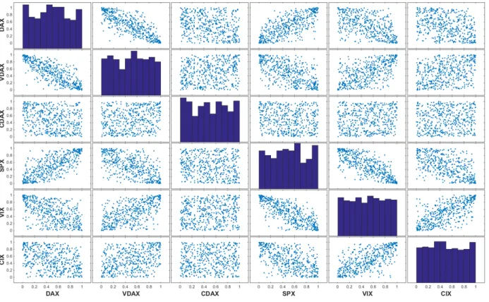
Figure 2: Filtered and transformed time-series.
Using the estimated parameters of the selected error distributions, we transformed the residuals to univariate uniform distributions so that only the multivariate dependencies remain. The bivariate scatter plots are shown in Figure2.
For the equity and volatility indices within each country we can clearly see the negative tail correlation. Also, DAX and SPX as well as VDAX and VIX show a positive tail dependence, even though it looks not as strong. When it comes to implied correlation the picture gets more ambivalent: while the CIX and SPX show negative tail dependence, it gets positive when looking at CIX and VIX conrming the industry-wide paradigm that in times of crisis, correlation goes up similar to volatility. However, the CDAX does not provide a clear picture even though one can still calculate a Pearson-correlation of−0.24
with the DAX and +0.21with the VDAX residuals. The weaker dependence compared
to the CIX could be explained by the DAX-implied correlation index showing a greater variability due to the fact that it is based on just about half the amount of single stocks. As we will see in the next section, it still holds important forecasting power for the VDAX.
4 VDAX forecasting based on implied correlation
Even though the study ofZhou(2013) indicates that implied correlation could hold some predictive power about its related equity index (and his realized volatility) this can only work to some extend if one believes in the ecient market hypothesis. However, as we will show in this section, it might be especially interesting for practitioners to use implied correlation indices for volatility forecasting. Therefore we model the logarithmic VDAX returns(rtVDAX)t∈Zby an ARMAX setup via
rtVDAX = a0+a1rVDAXt−1 +γ1r CDAX t−1 +γ2r VIX t−1 +γ3r CIX t−1 +εt+b1εt−1 (3) for t ∈ Z with (εt)t∈Z iid∼ (
0,1) and estimate this model under all possible parameter
restriction based on the rst 80% of our data time series. Afterwards the remaining 20% are used to evaluate the out of sample one-step forecasts, keeping the parameters xed, via their mean-squared-error (MSE) dened by
MSE= 1 n−m n ∑ i=m+1 [ ̂rVDAX t −r VDAX t ] 2 (4)
where n denotes the length of the whole time series while m is given by the training
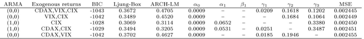
cuto (80% in our case). Of the 32 considered setups, the top 5 performers in terms of the MSE are listed in Table 3. In fact, the best presented model has also the lowest BIC. In general, we can see that the CDAX, VIX and CIX have a positive impact on the VDAX, conrming our ndings from the previous section. The inclusion of implied correlation indices improves volatility forecasting to a level which we were not able to reach with classical ARMA models even when allowing higher orders. Interestingly, one can see that although the top two performers do not include lagged VDAX returns, we are not able to nd any signicant autocorrelations or ARCH-eects in the error terms anymore.
ARMA Exogenous returns BIC Ljung-Box ARCH-LM α0 α1 β1 γ1 γ2 γ3 MSE (0,0) CDAX,VIX,CIX -1043 0.3672 0.4705 0.0009 − − 0.0209 0.1618 0.1202 0.002445
(0,0) VIX,CIX -1042 0.3489 0.4520 0.0009 − − − 0.1684 0.1064 0.002449
(1,0) CIX -1028 0.3069 0.3114 0.0009 0.0652 − − − 0.3380 0.002450
(1,0) CDAX,CIX -1029 0.3494 0.3205 0.0009 0.0531 − 0.0251 − 0.3487 0.002451
(0,0) CDAX,VIX -1042 0.3702 0.4627 0.0009 − − 0.0185 0.1946 − 0.002455
Table 3: ARMAX-models and out-of-sample prediction error measured by MSE
5 Concluding remarks
We calculated an implied correlation index for the German DAX and analyzed the depen-dence structure with its equity and volatility relatives as well as with the corresponding SPX related indices. Furthermore we have shown that the inclusion of implied corre-lation can eectively improve implied volatility forecasting. This leads to a potentially large amount of possible applications in derivative pricing, portfolio optimization as well as risk management and should further encourage exchanges to follow the CBOE and publish implied correlation, too.
References
Aboura, S., Chevallier, J., 2014. Volatility equicorrelation: A cross-market perspective. Economics Letters 122, 289295.
Barone-Adesi, G., Whaley, R. E., 1986. The valuation of American call options and the expected ex-dividend stock price decline. Journal of Financial Economics 17 (1), 91 111.
Barone-Adesi, G., Whaley, R. E., 1987. Ecient analytic approximation of American option values. The Journal of Finance 42 (2), 301320.
Black, F., Scholes, M., 1973. The pricing of options and corporate liabilities. The Journal of Political Economy, 637654.
Blair, B. J., Poon, S., Taylor, S. J., 2001. Modelling s&p 100 volatility: The information content of stock returns. Journal of Banking & Finance 25 (9), 16651679.
Campa, J. M., Chang, P. H. K., 1998. The forecasting ability of correlations implied in foreign exchange options. Journal of International Money and Finance 17 (6), 855880. Chicago Board Options Exchange, 2009. CBOE S&P 500 Implied Correlation
IndexAvail-able online: http://www.cboe.com/micro/impliedcorrelation/.
Christensen, B. J., Prabhala, N. R., 1998. The relation between implied and realized volatility. Journal of Financial Economics 50 (2), 125150.
Corrado, C. J., Miller Jr., T. W., 2005. The forecast quality of CBOE implied volatility indexes. Journal of Futures Markets 25 (4), 339373.
Deutsche Börse, 2007. Guide to the Volatility Indices of Deutsche BöerseAvailable online: http://www.dax-indices.com/EN/MediaLibrary/Document/VDAX_L_2_4_e.pdf. Driessen, J., Maenhout, P. J., Vilkov, G., 2009. The price of correlation risk: Evidence
Engle, R., 1988. Autoregressive conditional heteroscedasticity with estimates of the vari-ance of United Kingdom ination. Econometrica 96, 893920.
Fernandes, M., Medeiros, M. C., Scharth, M., 2014. Modeling and predicting the CBOE market volatility index. Journal of Banking & Finance 40, 110.
Fleming, J., 1998. The quality of market volatility forecasts implied by s&p 100 index option prices. Journal of Empirical Finance 5 (4), 317345.
Fleming, J., Ostdiek, B., Whaley, R. E., 1995. Predicting stock market volatility: a new measure. Journal of Futures Markets 15 (3), 265302.
Hansen, B. E., 1994. Autoregressive conditional density estimation. International Eco-nomic Review 35, 705730.
Härdle, W. K., Silyakova, E., 2012. Implied basket corre-lation dynamicsSFB 649 Discussion Paper. Available online: http://sfb649.wiwi.hu-berlin.de/papers/pdf/SFB649DP2012-066.pdf.
Linders, D., Schoutens, W., 2014. A framework for robust measurement of implied corre-lation. Journal of Computational and Applied Mathematics 271, 3952.
Ljung, G. M., Box, G. E. P., 1978. On a measure of a lack of t in time series models. Biometrika 65 (2), 297303.
Mittnik, S., 2014. VaR-implied tail-correlation matrices. Economics Letters 122 (1), 69 73.
Sheppard, K., 2013. MFE ToolboxAvailable online: https://www.kevinsheppard.com/MFE_Toolbox.
Siegel, A. F., 1997. International currency relationship information revealed by cross-option prices. Journal of Futures Markets 17 (4), 369384.
Skintzi, V. D., Refenes, A.-P. N., 2005. Implied correlation index: A new measure of diversication. Journal of Futures Markets 25 (2), 171197.
Walter, C. A., Lopez, J. A., 2000. Is implied correlation worth calculating? Evidence from foreign exchange options. The Journal of Derivatives 7 (3), 6581.
Zhou, H., 2013. On the predictive power of the implied correlation index.Working Paper. Available online: https://www2.bc.edu/~zhouho/JMP.pdf.