Asymmetric Properties of Office Rent Adjustment

(1)

Asymmetric Properties of Office Rent Adjustment

Dirk Brounen&Maarten Jennen

Published online: 20 May 2009

#The Author(s) 2009. This article is published with open access at Springerlink.com

Abstract In this paper we use an error correction model for understanding the changes in real office rents for a panel of 15 U.S. MSA’s over the period 1990-2007. We find that office rents in all cities react positively to a rise in office employment and lagged rent changes, while lagged deviations from equilibrium rent levels exhibit a slow and partial adjustment over time. Given the non-negativity constraint of vacancy rates we extend the basic model by examining whether rents react to positive changes in employment conditional on the vacancy rate level. Our results show that office rents react significantly stronger to increases in employment when vacancy rates are below the long-term average. We also repeat the analysis for clusters of cities based on similarities in rent and employment dynamics using multi dimensional scaling. The cluster results confirm the overall conclusions and show that our results are not solely valid for the full panel of cities.

Keywords Office rents . Error correction model . Panel data

Introduction

In this study we show that the impact of increases in demand for office space on changes in office rents depends on the disequilibrium in the demand-supply relationship. If vacancy rates are below their long term average office rents react significantly stronger to positive changes in office employment when compared to periods of abundant supply. Understanding rent dynamics is key to both users and investors in office markets, markets that have developed into a significant proportion of the overall economy. According to the U.S. Bureau of Labor Statistics office employment accounts for over 19% of non-farm employment. This statistic represents a total of 26 million office based employees DOI 10.1007/s11146-009-9188-9

D. Brounen

:

M. Jennen (*)

Rotterdam School of Management, Erasmus University, Burg. Oudlaan 50, 3062 PA, Rotterdam, The Netherlands

e-mail: mjennen@rsm.nl D. Brounen

e-mail: dbrounen@rsm.nl

M. Jennen

(2)

in the U.S. by the end of 2007. For metropolitan areas like San Francisco, Washington DC and New York the weight of office employment can reach peaks of close to 30%. Office rents are also a key input variable for construction decisions and to a large extent determine the profitability of new office investments. Hence, a vast strand of academic literature has developed over the years, which aims at cracking the DNA code of office rents. In these models, rents are typically related to changes in employment, office supply and vacancy levels. However, in almost all of these studies the authors assume that these relationships are symmetric, and thus that changes in employment will have similar scale effects irrespective of the level of the vacancy rate. Early studies by Wheaton (1987) already showed that vacancy rates evolve around a natural rate, and that given the non-negativity constraint vacancy rates tend to reach more distinctive peaks than troughs. Therefore, an increase in office employment, when vacancy rates are low, is likely to have a very different impact on rents, than when rates are high. Englund et al. (2008a) are the first to include these asymmetric properties into their model calibration. They explicitly studied asymmetric rent adjustments depending on the level of vacancy rates when modeling Stockholm office rents for the period 1977–2002 and reported a significant increase in the explanatory power of their rent models due to this inclusion. This paper will add to the existing literature by applying an asymmetric rent adjustment model to a unique panel set of quarterly data that covers fifteen metropolitan areas (MSA’s) in the United States over the period 1990–2007. Measured by net rentable area of office floor space these MSA’s are the largest in the U.S. and include Atlanta, Boston, Chicago, Dallas, Denver, Detroit, Houston, Los Angeles, Minneapolis, New York, Philadelphia, Pittsburgh, San Francisco and Washington DC. Besides a panel that includes all MSA’s in one specification we also estimate the model based on different clusters. We group MSA’s with multi dimensional scaling based on similarity in rent- or employment dynamics and run panel data regressions based on these clusters. The clustering methodology benefits from an increase in the number of observations when compared to analysis on a MSA level while keeping the in-group homogeneity as large as possible. Our results show that changes in office employment have a larger impact on office rents when vacancy rates are below their long term average. This finding implies for office investments that new demand does not influence rent rates in a symmetric way but is most influential when prevailing vacancy rates are relatively low. We also show that the coefficients are similar in sign and magnitude across clusters.

The paper continues as follows. After discussing the office market literature that is most relevant for our research, we discuss the rent adjustment model that will be applied in the subsequent analysis. Before discussing our results, we first present our dataset and review the main attributes of the markets that are included in our sample. In our results we explicitly compare results that were yielded from competitive model specifications; models with and without asymmetric properties. Besides discussing pooled panel results we also look at results, for clusters of cities. The main results will be summarized in our conclusions.

Modeling Office Rent Adjustments

The earliest office literature focused on vacancy rates and typically modelled office rent dynamics as a function of deviations from the natural vacancy rate that is

(3)

required to clear the market. Wheaton and Torto (1988) use U.S. national time series data on office rent levels and vacancy rates and find that excess vacancy rates affect real rents, while the natural vacancy rate is influenced by variables such as the local tenant structure, average lease terms in the market, expected absorption rates and operating costs. The main problem with this specification is the assumption that office rents keep on decreasing as long as the prevailing vacancy rate is above the perceived natural rate which does not fit actual relationships. Hendershott (1996), in a study of the Sydney office market, introduced a more general rent adjustment model in which changes in real rents are a function of vacancy and rent deviations from equilibrium levels. Equation1 shows the basic form of this type of real estate rent modelling. %ΔRt¼a vt vt1 þb R_t Rt1 ð1Þ Where vt* is the estimated natural vacancy rate and Rt* is the time-varying

equilibrium real office rent. This model offers a more general adjustment path for office rents with pleasing long-run properties, as effective rents are specified as adjustments to gaps between both the natural and actual vacancy rates and equilibrium and actual gross rents. With this equation, vacancy rates do not have to overshoot following a supply shock. After high vacancy rates have dragged rents significantly below equilibrium, the known eventual return to equilibrium acts as a force causing real rents to rise, even when the vacancy rate is still above the natural rate. This model is estimated by Hendershott et al. (1999) using data from the City of London for the period 1977-1996 and shows that the model tracks the market dynamics.

Hendershott et al. (2002) and Hendershott et al. (2002) extend these rent adjustment models by deriving a model that incorporates supply and demand factors within an Error Correction Model (ECM). This model is derived as a reduced-form estimation equation for the occupied office space and has the benefit that it does not require estimates for variables such as depreciation rates and operating expenses as is shown in Hendershott et al. (2002) where both a rent adjustment equation in line with Eq. 1 and an error correction model are estimated. Demand for space (D) is modelled as a function of real effective rent (R) and a proxy for office employment (E)1:

D¼l0R

l1_El2 ð₂Þ

Where theλi’s are constants with the price elasticity,λ1, expected to be negative

andλ2, the income elasticity, positive. Demand for office space, a function ofRand Eas in Eq.2, equals the product of available office space (SU) and one minus the prevailing office vacancy rate (v):

D Rð ;EÞ ¼ð1vÞSU ð3Þ Given the fact that real estate markets clear towards equilibrium through changes in rents and vacancy levels (as shown in Eq.3), vacancy enters the error correction model as a fitted variable indicated asbvin order to prevent endogeneity problems.

1

(4)

The procedure we use to model vacancy levels is in line with Hendershott et al. (2002) and consists of an AR(4) model based on quarterly observations. Adjusted R2 for the ten cities included in our analysis of the AR(4) model over the period 1990– 2006 range from 0.93 to 0.95. Rearranging Eqs. (2) and (3) by logarithmic transformation, including fitted vacancy levels, and extracting real rent levels results in Eq. (4).

lnRi;t¼g0þg1lnEi;tþg2lnb 1bvi;t

SUi:tc þui;t ð4Þ Where the subscriptsi and tdenote individual MSA’s and quarters respectively. The ECM which is used to model changes in real prime rents in a panel data approach estimates long run equilibrium relationships and short-term corrections. Due to frictions, as already indicated by Wheaton (1987) in a study of the cyclic behaviour of the U.S. office market, office markets usually do not clear within short-run periods of time. We measure this imbalance as the residual of Eq. 4 and subsequently introduce this variable as a factor in the short-run model. The rationale for including the residual in the rent adjustment model is the delay in restoration of equilibriums in real estate markets due to factors such as long term contracts and high search costs. Equation5shows the disequilibrium.

ui;t¼lnRi;tg0g1lnEi;tg2lnb 1bvi;t

SUi:tc ð5Þ Inclusion of the dependent variable in Eq. 5 in the rent adjustment model is possible if the variable is stationary which is equal to the independent variables being cointegrated. Since we base our model on panel data we apply the Levin et al. (2002) panel unit root test.2

Taking log differences of Eq. 4 and adding the stationary residual from Eq. 5

leads to the short-run rent adjustment model as depicted in Eq. 6 with an added lagged dependent variable to include the autoregression present in the change in real rent series.3 ΔlnRi;t¼a0þa1ΔlnEi;tþa2Δln 1bvi;t SUi;t þa3ui;t1 þa₄Δln R_i_;_t₁þ"i_;_t ð6Þ

According to Eq. (6) office rents react to short-run changes in causal variables and to lagged residuals of the long-run model, as a reflection of market imbalances.4The immediate responses to employment shocks and changes in occupied space are given by the coefficientsα1and α2.

We use an extended version of Eq. 6 to capture the asymmetry in office rent adjustments. By including an interaction term between changes in lnEtand a dummy

variable, that takes value 1 if the vacancy rate is below the MSA long term average

2

Tests for the presence of a unit root in the regression error terms shows that all residuals used in our study are stationary.

3

A regression of rent changes on rent changes lagged one period result in a coefficient of 0.32 which is significant at the 1% level.

4_{Modelling results are expected to indicate that}_α

0equals zero,α1,α2,α3andα5are positive, while,α4is

expected to display a negative sign.α3indicates the speed of adjustment towards equilibrium. Ifα3equals

−1 there is full equilibrium restoration after one period whileα3between zero and−1 or larger than−1

(5)

vacancy rate and the change in office employment positive, and 0 otherwise, we test the hypothesis that office rents react stronger to changes in office employment when the market is tight. This results in the following rent adjustment equation:

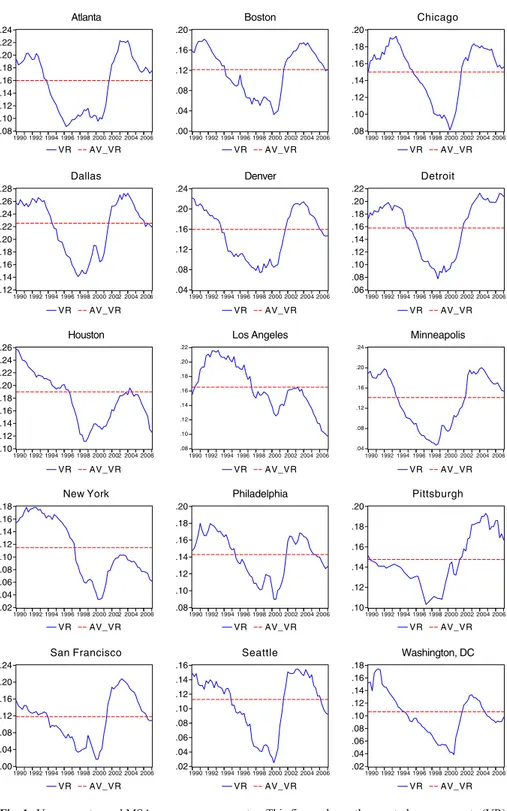
ΔlnRi;t¼a0þa1ΔlnEi;tþa2Δlnb 1bvi;t SUi;tc þa3ui;t1 þa4ΔlnRi;t1þa5 ΔlnEþi;t VR dummyi;tþ"i;t ð7Þ Figure1 shows for each MSA when the prevailing vacancy rate was above or below the local long term average vacancy rate. Our hypothesis is that the impact of office employment changes on rents is higher when vacancy rates are low when compared to a less tense office market.

We estimate and evaluate models (6) and (7) to test the effects of including the asymmetric properties based on our panel data of fifteen MSA’s over 69 quarters, resulting in a sample of 1035 observations. So far the office literature has been dominated by papers focusing on explaining the rent dynamics of one single office market. Examples are London by Wheaton, Torto and Evans (1997a), Hendershott et al. (1999), and Farelly and Sanderson Farrelly and Sanderson (2005), Stockholm by Gunnelin and Söderberg (2003), Englund et al. (2008a,b), Sydney by Hendershott (1996), San Francisco by Rosen (1984), Hong Kong by Hui and Yu (2006), Dublin by D’Arcy et al. (1999), and Boston by McClure (1991).

Few studies exist that analyze multiple markets. D’Arcy et al. (1997) examine 22 European cities and use pooled analysis with city dummies based on size of office stock, growth of real GDP and growth in service sector employment. Giussani et al. (1992) estimate rent models for ten European cities. Different demand side variables are tested in a pooled regression and for the individual cities. They find that coefficients are comparable in sign and magnitude across cities. Hendershott et al. (2002) estimate panel data error correction models for retail and office property rents for eleven regions in the U.K. covering 29 years. They estimate separate regional models and combine regions in panels based on communality in income and price elasticities. The main finding is that, while economic divers can vary between regions, that there is no evidence of differences in the operation of the regional property markets outside London. De Wit and van Dijk (2003) test rent models for static and dynamic panels for 46 office district across Asia, Europe and the U.S. and up to 56 quarterly observations per district.

Data

The data set in this study consists of quarterly, MSA level, real estate and employment data covering the period 1990-2007. Torto Wheaton Research (TWR) is the source of our real estate data which combines an extensive geographical coverage with a broad set of relevant real estate data. For the 15 largest office markets in the U.S. we have data on office completions, net absorption of office space, the net rentable area of office space in the MSA, office market vacancy rates and the TWR office rent index.5 Data on office completions reflects the square

5

The data gathering and compilation methodology of TWR has been discussed in detail in Wheaton et al. (1997b).

(6)

.08 .10 .12 .14 .16 .18 .20 .22 .24 1990 1992 1994 1996 1998 2000 2002 2004 2006

VR AV_VR VR AV_VR VR AV_VR

Atlanta .00 .04 .08 .12 .16 .20 1990 1992 1994 1996 1998 2000 2002 2004 2006 Boston .08 .10 .12 .14 .16 .18 .20 1990 1992 1994 1996 1998 2000 2002 2004 2006 Chicago .12 .14 .16 .18 .20 .22 .24 .26 .28 1990 1992 1994 1996 1998 2000 2002 2004 2006 Dallas .04 .08 .12 .16 .20 .24 1990 1992 1994 1996 1998 2000 2002 2004 2006 Denver .06 .08 .10 .12 .14 .16 .18 .20 .22 1990 1992 1994 1996 1998 2000 2002 2004 2006 Detroit .10 .12 .14 .16 .18 .20 .22 .24 .26 1990 1992 1994 1996 1998 2000 2002 2004 2006 Houston .08 .10 .12 .14 .16 .18 .20 .22 1990 1992 1994 1996 1998 2000 2002 2004 2006 Los Angeles .04 .08 .12 .16 .20 .24 1990 1992 1994 1996 1998 2000 2002 2004 2006 Minneapolis .02 .04 .06 .08 .10 .12 .14 .16 .18 1990 1992 1994 1996 1998 2000 2002 2004 2006 New York .08 .10 .12 .14 .16 .18 .20 1990 1992 1994 1996 1998 2000 2002 2004 2006 Philadelphia .10 .12 .14 .16 .18 .20 1990 1992 1994 1996 1998 2000 2002 2004 2006 Pittsburgh .00 .04 .08 .12 .16 .20 .24 1990 1992 1994 1996 1998 2000 2002 2004 2006 San Francisco .02 .04 .06 .08 .10 .12 .14 .16 1990 1992 1994 1996 1998 2000 2002 2004 2006 Seattle .02 .04 .06 .08 .10 .12 .14 .16 .18 1990 1992 1994 1996 1998 2000 2002 2004 2006 Washington, DC

Fig. 1 Vacancy rates and MSA average vacancy rates. This figure shows the quarterly vacancy rate (VR)

(7)

footage of office space completed each period or new space under construction due to completion in near future. The figure on net absorption reflects the net change in competitively leased space per period in square feet. The square footage is the amount of new space being brought into a market over a period of time, minus the change in vacant space over that same time period. Net rentable area data contain all office buildings whose size exceeds for most markets 20,000 or 30,000 square feet and results from information gathered by local CB Commercial offices throughout the United States. Information on office market vacancy rates is the result of an extensive survey by CB Commercial, which covers the vast majority of competitively rented buildings.

Different forms of office rent indices have been applied in extant literature. Private companies that provide the data apply different methodologies when constructing indices and face the problem of determining the true rent paid on a contract. This problem is caused by the incentive that property owners and tenants have not to disclose rent rates as this would limit future negotiation bandwidths. Furthermore, property owners offer all kinds of incentives in cash and kind to attract potential tenants. As the value of the incentives is positively related to the prevalent vacancy rate there is no fixed adjustment possible over time. McDonald (2002) discusses five different measures of rent per square foot that have been employed in empirical office market research and ranks the different rent indices in increasing accuracy as follows: [ I ] asking rent (gross and net), [ II ] face rent on new leases (gross and net), [ III ] consideration rent averaged over the term of the lease (rent levels are adjusted for broker commission and months of free rent but both on gross and net basis) [ IV ] consideration rent index (corrected for building and contract details) and [ V ] effective net rent that measures the net present value of cash flows over the term of the lease. The TWR office rent index that we use in our study is of type [ IV ] and is based on information contained in CB Commercial deals. Sivitanides (1997) and Mourouzi-Sivitanidou (2002) are examples of papers that use data by the same provider which is based on hedonic methodology as employed by Wheaton and Torto (1994) and Webb and Fisher (1996). Englund et al. (2008b) create a similar hedonic rent index for Stockholm for the period 1972-2002.

Being at the heart of the negotiations and deals provides CB Commercial with a broad set of contract and building details that subsequently enter the office rent index in the form of control variables. The basic rent specification equation is as follows:

logðRÞ ¼a0þa1SQFT þa2TERMþa3HIGHþa4NEWþa5GROSS

þXb_iDi 1993 i¼1979 þ30XdjSj 30 j¼1 ; ð8Þ where;

R total consideration rent per square foot per year SQFT square feet of lease

TERM length of the lease in years

HIGH dummy variable (1 for 5 + stories, 0 otherwise) NEW dummy variable (1 for new building, 0 otherwise) GROSS dummy variable (1 for gross rent, 0 otherwise)

(8)

Di dummy variable for each period

Sj dummy variable for up to 30 submarkets in MSA

The TWR rent index which is used in this study exhibits the rent for a five year, 10,000 ft gross rent lease in an existing building which is located in an average area in the MSA. The rent modeling presented in this study is based on real, instead of the reported nominal, rent levels. The U.S. Bureau of Labor Statistics provides consumer price indices (CPI) on a detailed MSA level which we use to adjust the nominal rent indices. The MSA level CPI is constructed with the first quarter of 1987 as base level, therefore all reported real rent levels are in Q1 1987 dollar values.

Our model of office rent changes builds upon changes in real estate variables and an office space demand factor. In line with existing literature we measure demand for office space as the number of people employed in office occupying industries. We gather employment data from the U.S. Bureau of Labor Statistics which provides a detailed overview of MSA level employment for a broad range of industry classifications. The definition of what employment sectors constitute office demand is not uniform across studies of office market dynamics. An extensive literature study of measures of office employment shows that most studies use employment in finance, insurance and real estate (FIRE), and service industries as a proxy for office employment. This type of office employment definition is used by for example Hekman (1985), Wheaton (1987), Wheaton et al. (1997b), Sivitanides (1997), Sivitanides (1998), Shilton (1998) Hendershott et al. (1999), Mourouzi-Sivitanidou (2002)6, Hendershott et al. (2002), Farrelly and Sanderson (2005), and Englund et al. (2008a,b). Other studies use a narrower approximation of office employment which only includes FIRE industries (see for example Rosen (1984), Hui and Yu (2006) and Pollakowski et al. (1992). Modeling office rents for small geographic areas such as financial heart of London (a.k.a.“The City”) or the financial district of Manhattan is probably well approximated with the narrower definition of office employment. However, for broader geographic areas, such as the MSA’s we use in this study, we propose the broader measure such as employed in the majority of office rent studies. Figure2 provides an overview of the industries that make up office employment according to the definition we use in this study.

The weight of professional and business service employment in total office employment, measured as the sum of FIRE and service sector employment, is on average 0.67 for all 15 MSA’s. The weight ranges between 0.58 for New York, a MSA with a strong financial and thus FIRE employment base, and 0.77 for Washington DC where services play a relatively large role. The service component of office employment increased for all MSA’s over the study period. The average change in FIRE employment is 21% between 1990 and 2007 (−8% in New York, up to 54% in Denver) while the average change in professional and business services is 54% (18% in Pittsburgh and 120% in Dallas). The average change across MSA’s in total office employment over our study period is 42%.

One potential problem with the office employment data is the strong seasonal component in the “administration and support and waste management and

6

She includes the ratio of FIRE to other office employment to take account on the idea that FIRE employment takes more square feet per employee.

(9)

remediation services” industry which works through to the overall office employment figure. In a perfect market companies would adjust their demand for space on a frequent basis; thereby minimizing rent costs. However, companies cannot adjust their space demand continuously due to moving costs, search time and long-term contracts. For this reason we expect companies to maximize their utility by renting floor space that lies somewhere between the maximum and minimum requirement to house all employees over contract duration. To overcome the impact of seasonality on our demand variable we use a four quarter moving average measure for the industry with high seasonal changes.7

Table 1 shows the correlation between changes in office employment for the whole country, the weighted average of MSA’s included in this study8, and the individual MSA’s.. The average correlation of changes in employment across all MSA’s is 0.48; reflecting strong differences in employment growth or composition across the sample. The table shows that the Atlanta, Detroit, Houston, Los Angeles and Pittsburgh are the MSA’s with on average the lowest correlation with other markets and that these are the only MSA’s that exhibit statistically non-significant correlations.

Office Employment

Financial Activities _{Business Services}Professional and

Finance and Insurance

Real Estate and Rental and Leasing

Credit intermediation and Related Activities Insurance Carriers and Related Activities Real Estate Professional, Scientific and Technical Services Management of Companies and Enterprises Admin., Support and Waste Mgt. and Remediation Services Architectural, Engineering and Related Services

Computer Systems Design and Related Services

Administrative and Support Services Employment Services Investigation and Security Services Services to Buildings and Dwellings Office Employment

Financial Activities _{Business Services}Professional and

Finance and Insurance

Real Estate and Rental and Leasing

Credit intermediation and Related Activities Insurance Carriers and Related Activities Real Estate Professional, Scientific and Technical Services Management of Companies and Enterprises Admin., Support and Waste Mgt. and Remediation Services Architectural, Engineering and Related Services

Computer Systems Design and Related Services

Administrative and Support Services Employment Services Investigation and Security Services Services to Buildings and Dwellings

Fig. 2 Office employment make-up. This figure shows the composition of office employment. Office

employment is defined as number of employees occupied in financial activities and professional and business services. Moving down through the figure each line combines the upper industry with the sub-industries it is composed of

7

We also tried the U.S. Statistics Bureau X12 procedure to delete the seasonality, but despite its theoretical superiority, peaks and troughs remain which does not fit demand for real estate assets.

8

(10)

T able 1 Co rrelation change in of fice empl oyment T otal _US 15 MSA s Atlanta Boston Chicago Dallas Denver Detro it Houston Los Angel es Minneapolis New York Philadelphi a Pittsb urg h San Francisco Se attle W ash ington, DC T otal U S 1 .829(** ) .656(**) .732(** ) .663(**) .763(** ) .653(**) .539(** ) .355(**) .473(** ) .545(** ) .704(** ) .670(**) .245(*) .618(** ) .693(** ) .554(** ) 15 MSAs .829(** ) 1 .642(**) .896(** ) .786(**) .831(** ) .725(**) .552(** ) .533(**) .640(** ) .673(** ) .910(** ) .734(**) .446(** ) .699(** ) .781(** ) .722(** ) A tlanta .656(** ) .642(** ) 1 .569(** ) .61 1(**) .568(** ) .591(**) .592(** ) 0.162 0.220 .484(** ) .481(** ) .417(**) 0.219 .439(** ) .450(** ) .339(** ) Bos ton .732(** ) .896(** ) .569(**) 1 .710(**) .681(** ) .674(**) .457(** ) .460(**) .499(** ) .664(** ) .827(** ) .620(**) .443(** ) .617(** ) .674(** ) .645(** ) Chi cago .663(** ) .786(** ) .61 1(**) .710(** ) 1 .666(** ) .659(**) .506(** ) .450(**) .370(** ) .589(** ) .601(** ) .588(**) .286(*) .498(** ) .580(** ) 459(**) D allas .763(** ) .831(** ) .568(**) .681(** ) .666(**) 1 .672(**) .430(** ) .605(**) .429(** ) .504(** ) .704(** ) .612(**) .331(** ) .676(** ) .751(** ) .490(** ) D enver .653(** ) .725(** ) .591(**) .674(** ) .659(**) .672(** ) 1 .468(** ) .491(**) .273(*) .583(** ) .571(** ) .454(**) .276(*) .658(** ) .682(** ) .3 79(** ) D etroit .539(** ) .552(** ) .592(**) .457(** ) .506(**) .430(** ) .468(**) 1 0.1 12 .342(** ) .432(** ) .354(** ) .279(*) 0.088 .340(** ) .359(** ) .297(* ) H ouston .355(** ) .533(** ) 0.162 .460(** ) .450(**) .605(** ) .491(**) 0.1 12 1 .275(*) .279(*) .399(** ) .412(**) 0.199 .522(** ) .569(** ) .298(*) Lo s Angele s .473(** ) .640(** ) 0.220 .499(** ) .370(**) .429(** ) .273(*) .342(** ) .275(*) 1 .297(*) .563(** ) .345(**) 0.131 .31 1(**) .401(** ) .449(** ) M inneapolis .545(** ) .673(** ) .484(**) .664(** ) .589(**) .504(** ) .583(**) .432(** ) .279(*) .297(*) 1 .593(** ) .424(**) .301(*) .481(** ) .541(* * ) .358(** ) N ew Y ork .704(** ) .910(** ) .481(**) .827(** ) .601(**) .704(** ) .571(**) .354(** ) .399(**) .563(** ) .593(** ) 1 .701(**) .480(** ) .551(** ) .674(** ) .706(** ) P hiladelphia .670(** ) .734(** ) .417(**) .620(** ) .588(**) .612(** ) .454(**) .279(*) .412(**) .345(** ) .424(** ) .701(** ) 1 .429(** ) .399(** ) .64 5(** ) .612(** ) P ittsburg h .245(*) .446(** ) 0.219 .443(** ) .286(*) .331(** ) .276(*) 0.088 0.199 0.131 .301(*) .480(** ) .429(**) 1 .280(*) .448(** ) .482(** ) S an Franc isco .618(** ) .699(** ) .439(**) .617(** ) .498(**) .676(** ) .658(**) .340(** ) .522(**) .31 1(**) .481(** ) .551(** ) .399(**) .280(*) 1 .64 5(** ) .456(** ) S eattle .693(** ) .781(** ) .450(**) .674(** ) .580(**) .751(** ) .682(**) .359(** ) .569(**) .401(** ) .541(** ) .674(** ) .645(**) .448(** ) .645(** ) 1 .491(** ) W ashington, DC .554(** ) .722(** ) .339(**) .645(** ) .459(**) .490(** ) .379(**) .297(*) .298(*) .449(** ) .358(** ) .706(** ) .612(**) .482(** ) .456(** ) .491(** ) 1 Th is table shows the correlation o f changes in of fice empl oyment betwe en pairs of MSA ’ s, the national change in of fice empl oyment (T otal U .S.) and an emp loym ent weigh ted ave rage of the 15 MS A ’ s inclu ded in the study (15 MS A ’ s). (**) and (*) indicate signif icance at 0.01 and 0.05 levels respec tively

(11)

Table 2 provides an overview of summary statistics of office data for the 15 MSA’s covered in this study. New York is by far the largest office market at the end of 2006 with a total square footage of over 400 million; over 60% larger than the second in line, Los Angeles and more than 6.5 times the size of Minneapolis which is the smallest office market covered in this study. Average real rents in 1987 constant dollars range between $9.7 in Houston and $24.4 in New York. Summary statistics for the vacancy rate show that all cities, when examining the mean over the study period, report double digit vacancy rates. Vacancy rates over the study period range between 1.7%, in San Francisco near the end of the Dotcom boom, to 30.3% in Houston towards the end of the 1980’s.

Figure3displays the time series of vacancy rates; real rent levels and the number of employees in office occupying industries over the period 1990-2007. The Figure shows that the vacancy rate for all MSA’s over the study period is often a close mirror image of real rent index despite the disturbing influence of new construction and hidden vacancy rates, as discussed in Englund et al. (2008b). Vacancy rates show similar patterns across all MSA’s and are characterized by high but steady levels over the years 1988-1994, which was a period characterized by a downturn in the U.S. economy partly due to the collapse of the junk bond market and a credit crunch. Over the whole, vacancy rates decreased over the period 1995-1998 preceding a period of low vacancy rates during the economic boom period 1998-2000. The latter period clearly shows the non-negativity constraint of vacancy rates as vacancies reached their local minima during the years 1998–2000, triggering new construction and the lowest space usage per employee over the study period as shown in Fig.4.9

After the turn of the millennium the U.S. economy hit hard times with the crash of the Dotcom bubble and the September 11 attacks on New York and Washington DC. The combination of ongoing new supply and decreasing employment at office occupying companies in all 15 MSA’s lead to a steep increase in vacancy rates over the period 2000–2003.

Real rent levels show similar patterns across MSA’s over time. Rent expressed in constant 1987 dollars show large dispersion across cities. In the first quarter of 2000 real rent levels were as low as $11.29 in Houston, which alternates with Denver for the lowest rent per square foot and as high as $28.51 in New York, where renting office space was most expensive over the whole study period. The discrepancy between the highest and lowest rent values is fairly consistent over time. On average the highest rent is 2.64 times the lowest rent over all quarters with a range of 2.1 to 3.6 over the study period.

Empirical Results

This section presents the results for the two stage error correction model for changes in real office rents. One of the contributions of this study is the addition of a test of asymmetry in rent response to positive changes in office employment. Therefore we

9

We measure space usage per employee in square feet as: (net rentable area*(1-vacancy rate))/office employment).

(12)

Table 2 Descriptive statistics

MSA Mean Min. Year / Quarter Min Max Year / Quarter Max

Panel A Atlanta 97,534 65,299 88Q1 126,691 07Q1 Boston 134,036 110,054 88Q1 154,920 07Q1 Chicago 193,125 160,835 88Q1 218,883 07Q1 Dallas 119,491 107,327 88Q1 139,324 07Q1 Denver 72,428 64,437 88Q1 85,372 07Q1 Detroit 62,018 50,664 88Q1 70,391 07Q1 Houston 127,040 121,447 88Q1 137,171 07Q1 Los Angeles 159,395 129,121 88Q1 173,390 07Q1 Minneapolis 57,723 47,998 88Q1 65,113 06Q4 New York 418,706 397,501 88Q1 427,568 07Q1 Philadelphia 87,196 68,891 88Q1 100,200 07Q1 Pittsburgh 59,027 53,050 88Q1 65,274 06Q4 San Francisco 73,119 63,071 88Q1 83,542 07Q1 Seattle 61,192 43,793 88Q1 75,599 07Q1 Washington, DC 211,601 159,481 88Q1 262,044 07Q1 All 128,909 43,793 427,568 Panel B Atlanta 11.6 10.0 93Q2 13.1 88Q2 Boston 17.0 12.8 92Q4 27.0 00Q4 Chicago 15.2 12.9 05Q3 18.3 88Q2 Dallas 11.0 9.1 93Q4 14.6 98Q4 Denver 9.8 8.2 91Q4 12.8 00Q2 Detroit 11.0 9.1 07Q1 14.1 88Q4 Houston 9.7 8.3 93Q4 11.6 00Q3 Los Angeles 13.6 11.3 95Q1 17.0 88Q1 Minneapolis 14.5 11.7 92Q4 18.3 88Q2 New York 24.4 18.3 93Q4 34.6 01Q1 Philadelphia 12.5 10.2 06Q3 16.2 89Q4 Pittsburgh 11.7 9.6 06Q3 13.1 00Q2 San Francisco 14.1 10.9 05Q1 23.1 00Q2 Seattle 14.3 12.2 04Q4 18.6 98Q4 Washington, DC 17.8 14.5 93Q2 23.5 00Q4 All 13.9 8.2 34.6 Panel C Atlanta 16.0% 8.7% 96Q2 22.3% 04Q1 Boston 12.1% 3.3% 00Q2 18.2% 91Q3 Chicago 15.0% 8.1% 00Q2 19.2% 93Q3 Dallas 22.5% 14.1% 97Q4 28.3% 88Q2 Denver 16.0% 7.4% 98Q3 27.3% 88Q1 Detroit 15.8% 7.8% 98Q4 21.3% 04Q1

(13)

estimate both a symmetric and an asymmetric model specification, based on Eqs.6

and 7 respectively. Table3 displays the results for the full panel including all 15 MSA’s. The top panel displays the results for the long run model. We base this model on non-differenced data and use it to calculate the prevailing rent disequilibrium.

The long run model does not differ between the symmetric and asymmetric model as it is merely used to determine the equilibrium rent level. Our regression results show that the long run model has an adjusted R-squared of approximately 0.80 with a Durbin Watson coefficient considerably below unity. The coefficients and model fit estimates from the long run model are comparable to the findings for European office markets as reported in Hendershott et al. (2002) and Brounen and Jennen (2009), and are a direct result of the trending variables used in the long-run model. The bottom panel in Table3 shows the result for the differenced rent model. In the symmetric model specification we show that rents react positively to changes in office employment and lagged changes in office rents. The coefficient for the error correction term is between zero and minus one which indicates a partial adjustment towards equilibrium over one quarter periods. The magnitude of this estimate is however very small, pointing at very slow adjustment over time.10The measure for occupied space shows an unexpected positive sign which is however only significant at the 5% level. The second short run model specification presented in Table3shows the result for the asymmetric model. Coefficients in the asymmetric model are similar to the results in the symmetric model in both sign and statistical significance, but with an even lower statistical significance for the occupied space variable. The

Table 2 (continued)

MSA Mean Min. Year / Quarter Min Max Year / Quarter Max

Houston 19.0% 11.2% 98Q3 30.3% 88Q1 Los Angeles 16.5% 9.7% 07Q1 21.6% 93Q2 Minneapolis 14.1% 4.7% 98Q3 21.9% 88Q3 New York 11.5% 3.3% 00Q2 17.9% 91Q2 Philadelphia 14.3% 9.0% 00Q3 18.0% 91Q1 Pittsburgh 14.7% 10.3% 97Q2 19.3% 04Q4 San Francisco 11.8% 1.7% 00Q1 20.8% 03Q2 Seattle 11.3% 2.5% 00Q2 17.2% 89Q2 Washington, DC 10.6% 3.9% 00Q4 17.4% 91Q2 All 14.7% 1.7% 30.3%

This table shows descriptive office market statistics for 15 U.S. MSA’s over the period 1988 till the first

quarter of 2007. Panel A shows descriptive statistics for net rentable area which is the sum of rentable

floor space of all office buildings in the MSA. Figures are in‘000s of square feet. Panel B shows summary

statistics of Torto Wheaton Research real rent (in 1987.1 constant dollars) per square foot. Panel C shows summary statistics for the vacancy rate

10

The error correction term is−0.008 in the symmetric model for the whole panel. This number implies

(14)

8 12 16 20 24 300 350 400 450 500 550 600 1990 1992 1994 1996 1998 2000 2002 2004 2006 1990 1992 1994 1996 1998 2000 2002 2004 2006 1990 1992 1994 1996 1998 2000 2002 2004 2006

VR REAL_RENT OE VR REAL_RENT OE VR REAL_RENT OE

1990 1992 1994 1996 1998 2000 2002 2004 2006 1990 1992 1994 1996 1998 2000 2002 2004 2006 1990 1992 1994 1996 1998 2000 2002 2004 2006

Atlanta 0 5 10 15 20 25 30 400 450 500 550 600 650 Boston 8 12 16 20 700 800 900 1000 1100 Chicago 8 12 16 20 24 28 300 400 500 600 700 Dallas 4 8 12 16 20 24 160 200 240 280 320 Denver 4 8 12 16 20 24 360 400 440 480 520 560 Detroit 8 12 16 20 24 28 300 350 400 450 500 550 Houston 8 12 16 20 24 900 1000 1100 1200 1300 Los Angeles 4 8 12 16 20 24 280 320 360 400 440 Minneapolis 0 10 20 30 40 1700 1800 1900 2000 2100 2200 New York 8 10 12 14 16 18 20 480 520 560 600 640 680 Philadelphia 8 10 12 14 16 18 20 180 190 200 210 220 Pittsburgh 0 5 10 15 20 25 400 440 480 520 560 600 San Francisco 0 4 8 12 16 20 200 240 280 320 360 Seattle 0 5 10 15 20 25 400 500 600 700 800 900 Washington, DC

Fig. 3 Office market dynamics. This figure shows the dynamics in vacancy rate (VR, left axis in %), the

Torto Wheaton Research office rent index in real terms (Real_rent, left axis in constant 1987.1 dollars) in

$ per square foot and office employment (OE, right axis in‘000s employees) for all 15 MSA’s covered in

(15)

8 12 16 20 24 170 180 190 200 210 1990 1992 1994 1996 1998 2000 2002 2004 2006

VR FT2_PER_EMPLOYEE VR FT2_PER_EMPLOYEE VR FT2_PER_EMPLOYEE

Atlanta 0 4 8 12 16 20 200 210 220 230 240 250 260 1990 1992 1994 1996 1998 2000 2002 2004 2006 Boston 8 12 16 20 165 170 175 180 185 190 195 1990 1992 1994 1996 1998 2000 2002 2004 2006 1990 1992 1994 1996 1998 2000 2002 2004 2006

1990 1992 1994 1996 1998 2000 2002 2004 2006 1990 1992 1994 1996 1998 2000 2002 2004 2006

1990 1992 1994 1996 1998 2000 2002 2004 2006

1990 1992 1994 1996 1998 2000 2002 2004 2006 1990 1992 1994 1996 1998 2000 2002 2004 2006

1990 1992 1994 1996 1998 2000 2002 2004 2006

1990 1992 1994 1996 1998 2000 2002 2004 2006 1990 1992 1994 1996 1998 2000 2002 2004 2006

1990 1992 1994 1996 1998 2000 2002 2004 2006

1990 1992 1994 1996 1998 2000 2002 2004 2006 1990 1992 1994 1996 1998 2000 2002 2004 2006 Chicago 12 16 20 24 28 160 180 200 220 240 Dallas 4 8 12 16 20 24 220 230 240 250 260 270 Denver 4 8 12 16 20 24 108 112 116 120 124 Detroit 8 12 16 20 24 28 220 240 260 280 300 Houston 8 12 16 20 24 112 116 120 124 128 Los Angeles 4 8 12 16 20 24 132 136 140 144 148 152 Minneapolis 0 4 8 12 16 20 175 180 185 190 195 200 205 New York 8 10 12 14 16 18 20 124 128 132 136 140 144 Philadelphia 10 12 14 16 18 20 ₂₄₀245 250 255 260 265 270 Pittsburgh 0 5 10 15 20 25 124 128 132 136 140 144 148 San Francisco 0 4 8 12 16 185 190 195 200 205 210 215 Seattle 0 4 8 12 16 20 260 280 300 320 340 360 Washington, DC

Fig. 4 Occupied office space per office employee. This figure shows vacancy rate dynamics (VR, left

axis in %) and the office space usage per employee (FT2_per_employee, left axis in ft2per employee)

(16)

Table 3 Regression results (all cities)

All City Panel

Symmetric Model Asymmetric Model

Long-run model Constant 8.559 *** 8.559 *** (0.968) (0.968) ln (Et) 1.292 *** 1.292 *** (0.095) (0.095) ln [(1−v^t)SUt] −1.225 *** −1.225 *** (0.132) (0.132) N 990 990 R2_-adj _0.799 _0.799 DW 0.060 0.060 Short-run model Constant −0.002 *** −0.003 *** (0.000) (0.000) Δln (Et) 2.499 *** 1.503 *** (0.272) (0.314) Δln [(1−v^t)SUt] 0.584 ** 0.156 * (0.279) (0.275) ut-1 −0.008 *** −0.015 *** (0.002) (0.002) Δln Rt-1 −0.419 *** 0.399 *** (0.030) (0.029) [Δln E +t] * VR_DUMMYt — 2.406 *** (0.401) N 975 975 R2_-adj _0.399 _0.421 DW 1.913 1.918

This table reports the error correction model of office rents for a panel of 15 MSA’s included in the study

based on quarterly observations over the period 1990–2007. The long-run model lnRt=α0+α1lnEt+

α2ln[1-v^t]SUtis estimated as a cross sectional fixed effect model.The dependent variable is real office

rent in 1987.1 constant U.S. dollars. We estimate office employment (Et) as the sum of employment in

finance, insurance, real estate, professional- and business services.[1−v^t]SUtis an estimate for occupied

space, wherev^is the fitted vacancy rate based on an AR(4) model andSUis the supply of office space in

square feet. The results include the symmetric and asymmetric models which differ in the short-run model

only. The symmetric short-run model∆lnRt=α0+α1∆lnEt+α2∆ln[1−v^t]SUt t+α3ut−1+α4∆lnRt−1is

estimated as a cross sectional fixed effect model.Δmeasures the one period change in variables.ut−1is

the one period lagged residual of the long-run model.∆lnRt−1is the one period lagged change in real

prime rents. The asymmetric short-run model∆lnRt =α0 +α1∆lnEt +α2∆ln[1−v^t ]SUt +α3ut−1 +

α4∆lnRt−1+α5[∆lnE +t]VR_DUMMYtis estimated as a cross sectional fixed effect model. [∆lnE +t]

reflects positive one period changes in office employment and takes value zero is the change in

employment is negative. VR_DUMMYtis a dummy variable that takes value 1 if the vacancy rate in timet

is below the MSA average vacancy rate, and 0 otherwise. DW is the Durbin-Watson statistic. Standard error statistics appear in parentheses. ***, **, * indicate significance at the 1%, 5% and 10% level respectively

(17)

positive and significant coefficient for the asymmetry variable shows that rents react significantly stronger to positive changes in office employment when vacancy rates are below the long term average, when compared to times of abundant vacant space. This finding is in line with expectations. If vacancy rates are high, new demand for space will first alleviate the owners of non-income producing vacant space before a clear effect on office rents is visible. When vacancy rates are low the effect of additional demand for office space as a result of an increase in office employment is more directly related to office rents. However, including this asymmetric element in the model enhances the fit of the model only marginally.

Cluster Analysis

The panel results presented in Table 3 assume that the coefficients for the independent variables are equal across all MSA’s. In order to relax this assumption we create panels based on similarity in the pattern of rent and office employment changes over the sample period. In this way we are able to maintain the benefit of large sample sizes, examine clusters with maximum between cluster heterogeneity, while keeping the within sample homogeneity as large as possible. Hendershott et al. (2002) is the only other known study that groups regions based on some similarity. Their paper studies rent changes for a range of regions and estimates separate models for“London”and“Other”regions in the UK for 11 regions and 29 years. Clusters in the Hendershott et al. (2002) paper are based on similarities of the income and price elasticities in the long run models. In this study we use an alternative methodology in which we use multi dimensional scaling (MDS) and subsequent hierarchical clustering analysis to group MSA in two clusters based on similarities in changes in rent and office employment over time. MDS is a powerful tool for visualizing correlations between pairs of cities or other instances (see for example Groenen and Franses (2000) for an application in stock market correlation analysis). MDS creates points in a low dimensional space where each dot reflects for example a city. Clusters of cities appear if dots in the low dimensional space appear close to each other in the output. The benefit over more traditional correlation analysis is the way MDS shows not only the similarity between individual pairs of instances but also the way in which all other observations are related. Besides the visual application, MDS output also includes common space coordinates which forms the input for the geographic representation of similarities. The common space coordinates form the input for hierarchical clustering analysis; the foundation for the actual cluster formation. We test different dimensional settings for the MDS and found, according to the guidelines by Kruskal (1964), that the use of three dimensions is optimal in our study. Our clusters based on communalities in rent and office employment changes over the study period are shown in Fig.4. Panels A and B show the clusters based on rent and employment changes, respectively. Based on real rent changes we form two clusters. One cluster consists of Boston, New York and San Francisco (further indicated as cluster A2) and the other cluster encompasses all other MSA’s (cluster A1).

If we base the clusters on office employment changes, Fig.5 shows that three main clusters arise. One cluster consists of Atlanta and Detroit (cluster B3), a second

(18)

cluster includes New York, Philadelphia, Pittsburg, Los Angeles and Washington DC (cluster B2) and the third cluster consists of the remaining MSA’s (cluster B1).11 Panel A1 in Table4 shows the results for cluster A1. Coefficients and signs are comparable to the findings presented in Table3with a model fit that is slightly lower than the result for a panel including all MSA’s. The error correction term shows that rent very slowly adjust towards equilibrium over the term of one quarter; a finding shared with all other model specifications presented in this study. Results of the short run model show that the impact of changes in our estimate of occupied space is not statistically different from zero. Again, we show that the rent adjustment as a result

Fig. 5 Hierarchical clusters. This figure shows the dendrogram which results after a hierarchical

clustering analysis based on three dimensional common space coordinates. Common space coordinates are constructed with multi dimensional scaling. Panel A shows clusters based on changes in office rents and Panel B shows clusters based on changes in office employment

11_{One interesting finding from this clustering methodology based on similarities in office rent or}

employment changes is that clusters are not in line with geographic locations of the MSA’s. Further

analysis could provide more insight into the driving forces behind the correlations; possible causes are similarities in local GDP drivers or employment composition.

(19)

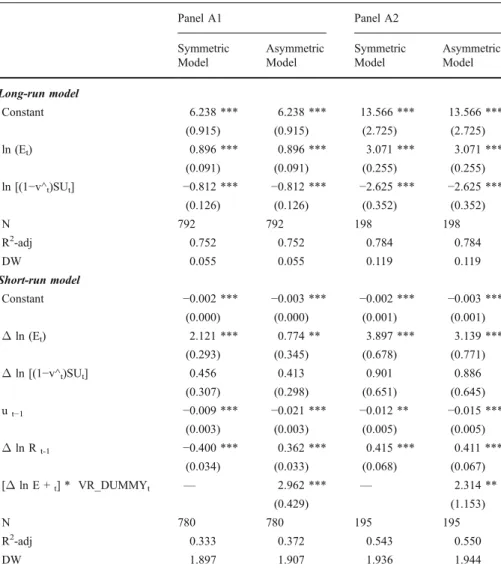
Table 4 Regression results for clusters based on communality in office rent changes Panel A1 Panel A2 Symmetric Model Asymmetric Model Symmetric Model Asymmetric Model Long-run model Constant 6.238 *** 6.238 *** 13.566 *** 13.566 *** (0.915) (0.915) (2.725) (2.725) ln (Et) 0.896 *** 0.896 *** 3.071 *** 3.071 *** (0.091) (0.091) (0.255) (0.255) ln [(1−v^t)SUt] −0.812 *** −0.812 *** −2.625 *** −2.625 *** (0.126) (0.126) (0.352) (0.352) N 792 792 198 198 R2_-adj _0.752 _0.752 _0.784 _0.784 DW 0.055 0.055 0.119 0.119 Short-run model Constant −0.002 *** −0.003 *** −0.002 *** −0.003 *** (0.000) (0.000) (0.001) (0.001) Δln (Et) 2.121 *** 0.774 ** 3.897 *** 3.139 *** (0.293) (0.345) (0.678) (0.771) Δln [(1−v^t)SUt] 0.456 0.413 0.901 0.886 (0.307) (0.298) (0.651) (0.645) ut−1 −0.009 *** −0.021 *** −0.012 ** −0.015 *** (0.003) (0.003) (0.005) (0.005) Δln Rt-1 −0.400 *** 0.362 *** 0.415 *** 0.411 *** (0.034) (0.033) (0.068) (0.067) [Δln E +t] * VR_DUMMYt — 2.962 *** — 2.314 ** (0.429) (1.153) N 780 780 195 195 R2_-adj _0.333 _0.372 _0.543 _0.550 DW 1.897 1.907 1.936 1.944

This table reports the error correction model of office rents for a panel of 15 MSA’s included in the study based on

quarterly observations over the period 1990–2007. The sample is split in two Panels based on communality in

office rent changes. The long-run model lnRt=α0+α1lnEt+α2ln[1−v^t]SUtis estimated as a cross sectional

fixed effect model.The dependent variable is real office rent in 1987.1 constant U.S. dollars. We estimate office

employment (Et) as the sum of employment in finance, insurance, real estate, professional- and business

services.[1−v^t]SUtis an estimate for occupied space, wherev^tis the fitted vacancy rate based on an AR(4)

model andSUtis the supply of office space in square feet. The results include the symmetric and asymmetric

models which differ in the short-run model only. The symmetric short-run model∆lnRt=α0+α1∆lnEt+α2∆ln

[1−v^t]SUt t+α3ut−1+α4∆lnRt−1is estimated as a cross sectional fixed effect model.Δmeasures the one

period change in variables.ut−1is the one period lagged residual of the long-run model.∆lnRt−1is the one

period lagged change in real prime rents. The asymmetric short-run model∆lnRt=α0+α1∆lnEt+α2∆ln[1−v^t]

SUt+α3ut−1 α4∆lnRt−1+α5[∆lnE +t]VR_DUMMYtis estimated as a cross sectional fixed effect model.

[∆lnE +t] reflects positive one period changes in office employment and takes value zero is the change in

employment is negative. VR_DUMMYtis a dummy variable that takes value 1 if the vacancy rate in timetis

below the MSA average vacancy rate, and 0 otherwise. DW is the Durbin-Watson statistic. Standard error statistics appear in parentheses. ***, **, * indicate significance at the 1%, 5% and 10% level respectively

(20)

T able 5 Re gression res ults for clus ters based on com munality in of fice emp loyment changes Pa nel B1 Panel B2 Panel B3 Sym metric Model Asymm etric Model Symme tric Mod el Asymm etric Mod el Symme tric Mod el Asymm etric Mod el Lo ng-ru n model Co nstant 8.845 *** 8.84 5 *** 8.98 4 *** 8.98 4 *** 7.55 2 *** 7.552 *** 1.337 1.73 3 1.73 3 1.19 0 1.19 0 ln (E t ) 1.291 *** 1.29 1 *** 1.25 1 *** 1.25 1 *** 1.02 5 *** 1.025 *** 0.126 0.12 6 0.16 9 0.16 9 0.15 7 0.157 ln [(1 − v^ t )SU t ] − 1.247 *** − 1.24 7 *** − 1.22 6 *** − 1.22 6 *** − 1.02 9 *** − 1.029 *** 0.179 0.17 9 0.23 3 0.23 3 0.18 9 0.189 N 552 552 345 345 138 138 R 2-adj 0.684 0.68 4 0.87 2 0.87 2 0.36 6 0.366 DW 0.058 0.05 8 0.07 5 0.07 5 0.14 6 0.146 Sh ort-run mode l Co nstant − 0.003 *** − 0.00 3 *** − 0.00 2 *** − 0.00 3 *** − 0.00 2 * * − 0.002 ** 0.000 0.00 0 0.00 1 0.00 1 0.00 1 0.001 Δ ln (E t ) 2.549 *** 1.70 7 *** 3.22 5 *** 1.70 3 * * 1.29 9 * * 0.969 0.382 0.48 2 0.57 9 0.82 9 0.60 1 0.748

(21)

Panel B1 Panel B2 Panel B3 Symme tric Model Asymm etric Model Sym metric Mod el Asymm etric Mod el Symme tric Mod el A symmetric Mod el Δ ln [(1-v^ t )SU t ] 0.663 * 0.591 0.97 9 * 0.82 6 0.57 7 0.579 0.382 0.379 0.55 3 0.55 2 0.77 2 0.773 ut − 1 − 0.013 *** − 0.016 *** − 0.00 4 − 0.00 8 * − 0.01 8 * − 0.020 * 0.003 0.003 0.00 4 0.00 5 0.01 1 0.01 1 Δ ln R t − 1 − 0.464 *** 0.456 *** 0.32 5 *** 0.30 6 *** 0.25 9 *** 0.254 *** 0.042 0.041 0.05 5 0.05 5 0.08 7 0.087 [ Δ ln E + t ] * VR_ DUMM Yt — 1.586 *** — 2.48 1 * * — 0.593 0.560 0.97 5 0.798 N 520 520 325 325 130 130 R 2-ad j 0.463 0.469 0.30 7 0.31 8 0.18 9 0.187 D W 1.795 1.809 1.98 1 1.96 9 1.57 2 1.581 This table reports the error cor rection model of of fice rents for a pan el of 15 MSA ’ s inclu ded in the study base d o n qua rterly observa tions ove r the per iod 1990 – 2007 . T h e sam ple is split in tw o Panels based on com munality in of fice emp loym ent cha nges. Th e long-run model ln Rt = α0 + α1 ln Et + α2 ln[ 1 − v^ t ] SU t is estim ated as a cro ss sectiona l fixed eff ect model . The depend ent var iable is real of fice rent in 1987 .1 constan t U.S. dollars. W e estim ate of fice employm ent ( Et ) as the sum of emp loym ent in fina nce, insurance, real esta te, professional-and busin ess ser vices. [1 − v^t ]SU t is an estimate for occ upied spac e, where v^t is the fitted vacan cy rate based on an A R(4) model and SU t is the supp ly of of fice space in square feet. The results inclu de the symm etric and asym metric mode ls which dif fer in the shor t-run mode l only . T h e symm etric shor t-run mode l ∆ ln Rt = α0 + α1 ∆ ln Et + α2 ∆ ln[1 − v^t ] SU tt + α3 ut− 1 + α4 ∆ ln Rt− 1 is estim ated as a cro ss sectiona l fixed ef fect model. Δ measur es the one per iod change in variables. ut− 1 is the one period lagged residual of th e long-run mode l. ∆ ln Rt− 1 is the one period lagg ed change in real prim e rents. The asym metric short-run mode l ∆ ln Rt = α0 + α1 ∆ ln Et + α2 ∆ ln[1 − v^t ] SU t + α3 ut− 1 + α4 ∆ ln Rt− 1 + α5 [ ∆ ln E+ t ]VR_DU MMY t is estim ated as a cross sec tional fixed ef fect model. [ ∆ ln E+ t ] reflects positiv e one period change s in o ffice employm ent and take s valu e zero is the cha nge in emp loym ent is negative. VR_ DUMM Yt is a dummy variable that takes valu e 1 if the vacan cy rate in time t is below the MS A average vacancy rate, and 0 otherwise. D W is the Durb in-W atso n statistic. Sta ndard err or statistics appea r in parentheses. ***, **, * indicate signif icance at the 1%, 5% and 10% level respecti vely

(22)

of an increase in office employment, the asymmetric model specification, is stronger when vacancy rates are below their long term averages. The results for the remaining MSA’s, as presented under Panel A2 in Table4, are largely comparable in sign and magnitude with a strong increase in model fit when compared to the panel of all MSA and panel A1.

Table5 shows the results for the clusters based on communalities in changes in office employment across MSA’s. Panels B1 and B2 are comparable to the results presented in Tables 3 and 4. Overall we find that all included variables are statistically significant with expected signs but also show that the variable that measures occupied space is hardly or not significant. Panel B3 stands out with model fit considerably below the other model specifications in both the long-run and the short-run model. Changes in office employment, office demand and the asymmetry measure are not significant for asymmetric model specification presented for cluster B3 while they are for most other specifications.

Conclusion

In this paper we use an error correction model for understanding the changes in real office rents for a panel of 15 U.S. MSA’s over the period 1990–2007. We find that office rents react positively to a rise in office employment, lagged changes in office rents and that there is only very slow error correction towards estimated equilibrium rents. Given the non-negativity constraint of vacancy rates we extend the model by examining whether rents react to changes in employment conditional on the vacancy rate. Our results show that office rents react significantly stronger to increases in employment when vacancy rates are below the long-term average. We relax the assumption that all MSA’s exhibit the same reaction to changes in independent variables by introducing results based on clustering. We base clusters on similarities in changes in rent and office employment with multi dimensional scaling. Generally we find that there are large differences in model fit across the clusters we examined but that there are only small and insignificant differences in coefficients across clusters. We thus conclude that the cluster results confirm the results found for the panel that includes all MSA’s.

Acknowledgements The authors would like to thank Peter Englund and other participants in the

Cambridge-UNC Charlotte-Amsterdam Symposium 2008 in Amsterdam, for their helpful feedback. Furthermore we would like to thank the editors of the JREFE Special Issue, Richard Buttimer, Erasmo Giambona and Kanak Patel for their comments. We are grateful to Torto Wheaton Research for sharing their valuable data with us.

Open Access This article is distributed under the terms of the Creative Commons Attribution

Noncommercial License which permits any noncommercial use, distribution, and reproduction in any medium, provided the original author(s) and source are credited.

References

Brounen, D., & Jennen M. (2009), Office rent determinants: a tale of ten cities,Journal of Real Estate

Finance and Economics, forthcoming.

D’Arcy, E., McGough, T., & Tsolacos, S. (1997). National economic trends, market size and city growth

(23)

D’Arcy, E., McGough, T., & Tsolacos, S. (1999). An econometric analysis and forecasts of the office

rental cycle in the Dublin area.Journal of Property Research, 16(4), 309–321.

De Wit, I., & van Dijk, R. (2003). The global determinants of direct office real estate returns.Journal of

Real Estate Finance and Economics, 26(1), 27–45.

Englund P., Gunnelin Å., Hendershott P. H., & Söderberg B. (2008a), Asymmetries in property space

market adjustment,Paper presented at the Rotterdam School of Management real estate symposium.

Englund, P., Gunnelin, Å., Hendershott, P. H., & Söderberg, B. (2008b). Adjustment in property space

markets: taking long-term leases and transaction costs seriously.Real Estate Economics, 36(1), 81–

109.

Farrelly, K., & Sanderson, B. (2005). Modeling regime shifts in the city of London office rental cycle.

Journal of Property Research, 22(4), 325–344.

Giussani, B., Hsia, M., & Tsolacos, S. (1992). A comparative analysis of the major determinants of office

rental values in Europe.Journal of Property Valuation and Investment, 11, 157–173.

Groenen, P. J. F., & Franses, P. H. (2000). Visualizing time-varying correlations across stock markets.

Journal of Empirical Finance, 7, 155–172.

Gunnelin, Å., & Söderberg, B. (2003). Term structures in the office rental market in Stockholm.Journal of

Real Estate Finance and Economics, 26(2/3), 241–265.

Hekman, J. S. (1985). Rental price adjustments and investment in the office market.AREUEA Journal, 13

(1), 32–47.

Hendershott, P. H. (1996). Rental adjustment and valuation in overbuilt markets: Evidence from the

Sydney office market.Journal of Urban Economics, 39, 51–67.

Hendershott, P. H., Lizieri, C. M., & Matysiak, G. A. (1999). The Workings of the London office market.

Real Estate Economics, 27(2), 365–387.

Hendershott, P. H., MacGregor, B., & White, M. (2002). Explaining real commercial rents using an error

correction model with panel data.Journal of Real Estate Finance and Economics, 24(1/2), 59–87.

Hui, E. C. M., & Yu, K. H. (2006). The dynamics of Hong Kong’s office rental market.International

Journal of Strategic Property Management, 10, 145–168.

Kruskal, J. B. (1964). Multidimensional scaling by optimizing goodness of fit to a nonmetric hypothesis.

Psychometrika, 29(1), 1–27.

Levin, A., Lin, C. F., & Chu, S. S. (2002). Unit root tests in panel data: Asymptotic and finite sample

properties.Journal of Econometrics, 108, 1–24.

McClure, K. (1991). Estimating occupied office space: comparing alternative forecast methodologies.The

Journal of Real Estate Research, 6(3), 305–314.

McDonald, J. F. (2002). A survey of econometric models of office markets.Journal of Real Estate

Literature, 10(2), 223–242.

Mourouzi-Sivitanidou, R. (2002). Office rent processes: The case of U.S. metropolitan markets.Real

Estate Economics, 30(2), 317–344.

Pollakowski, H. O., Wachter, S. M., & Lynford, L. (1992). Did office market size matter in the 1980s? A

time-series cross sectional analysis of metropolitan area office markets. AREUEA Journal, 20(1),

303–324.

Rosen, K. T. (1984). Toward a model of the office building sector.AREUEA Journal, 12(3), 261–269.

Shilton, L. (1998). Patterns of office employment cycles.Journal of Real Estate Research, 15(3), 339–

354.

Sivitanides, P. S. (1997). The rent adjustment process and the structural vacancy rate in the commercial

real estate market.Journal of Real Estate Research, 13(2), 195–209.

Sivitanides, P. S. (1998). Predicting office returns: 1997–2001.Real Estate Finance, 15(1), 33–42.

Webb, R. B., & Fisher, J. D. (1996). Development of an effective rent (lease) index for the Chicage CBD.

Journal of Urban Economics, 39(1), 1–19.

Wheaton, W. C. (1987). The cyclic behavior of the national office market.AREUEA Journal, 15(4), 281–

299.

Wheaton, W. C., & Torto, R. G. (1988). Vacancy rates and the future of office rents.Journal of the

American Real Estate and Urban Economics Association, 16(4), 430–436.

Wheaton, W. C., & Torto, R. G. (1994). Office rent indices and their behavior over time.Journal of Urban

Economics, 35(2), 121–139.

Wheaton, W. C., Torto, R. G., & Evans, P. (1997a). The cyclic behavior of the Greater London office

market.Journal of Real Estate Finance and Economics, 15(1), 77–92.

Wheaton, W. C., Torto, R. G., & Southard, J. A. (1997b). The CB Commercial/Torto Wheaton Database.