Fast Speaker Recognition using Efficient Feature Extraction Technique

(1)

Fast Speaker Recognition using Efficient Feature Extraction

Technique

1

Sejal Shah, 2Archana Bhise

1

Electronics Department, Mumbai University, K. J. Somaiya Institute of Engineering and Information Technology Mumbai, Maharashtra, India

2

Electronics and Telecommunications Department, Mumbai University, K. J. Somaiya Institute of Engineering and Information Technology

Mumbai, Maharshtra, India

Abstract

Digital processing of speech signal and speaker recognition algorithm is very important for fast and accurate automatic voice recognition technology. A direct analysis of the voice signal is complex due to too much information contained in the signal. Therefore the digital signal processes such as Feature Extraction and Feature Matching are introduced to represent the voice signal. The non-parametric method for modeling the human auditory perception system, Mel Frequency Cepstral Coefficients (MFCCs) is utilized as extraction technique. MFCC imitates the human hearing system; therefore it provides better recognition rates than Linear Predictive Coefficients (LPC). For the present work, work, the non linear sequence alignment known as Dynamic Time Warping (DTW) is used as features matching technique. Since voice signal tends to have different temporal rate, the alignment is important to produce better performance. This paper presents the viability of MFCC to extract features of speech signal and DTW to compare the corresponding test patterns.

Keywords:Dynamic Time Warping (DTW). Hamming Window, Mel filter banks

1. Introduction

Voice Signal identification consists of the process of converting a speech waveform into features that are useful for further processing. There are many algorithms and techniques that are used. It depends on features capability to capture time, frequency and energy and convert into set of coefficients for cepstrum analysis. Generally, human voice conveys information such as gender, emotion and identity of the speaker. The objective of speaker recognition is to determine which speaker is present based on the individual’s utterance. Several techniques have been proposed for reducing the mismatch between the testing and training environments [1]. Many of these methods operate either in spectral or in cepstral domain. Human voice is converted into digital signal form to produce digital data representing each level of signal at every discrete time step. The digitized speech samples are

then processed using (Mel Frequency Cepstrum Coefficients) MFCC [3] to produce voice features. After that, the coefficients of voice features go through DTW (Dynamic Time Warping) algorithm [7] to select the pattern that matches with any one from the database and input sample which gives least distance.

The rest of the paper is organized as follows: principles of speaker recognition is given in section II, the methodology of the study is provided in section III, which is followed by result and discussion in section IV, and finally concluding remarks are given in section V.

2. Speaker Recognition

Anatomical structure of the vocal tract is unique for every person and hence the voice information available in the speech signal can be used to identify the speaker. Recognizing a person by her/his voice is known as speaker recognition. Since differences in the anatomical structure are an intrinsic property of the speaker, voice comes under the category of biometric identity. Using voice for identity has several advantages. One of the major advantages is remote person authentication. Like any other pattern recognition systems, speaker recognition systems also involve two phases namely, training and testing [1]. Training is the process of similarizing the system with the voice characteristics of the speakers registered. Testing is the actual recognition task. The block diagram of training phase is shown in Fig.1. Feature vectors representing the voice characteristics of the speaker are extracted from the training utterances and are used for building the reference models. During testing, similar feature vectors are extracted from the test utterance, and the degree of their match with the reference is obtained using some matching technique. The level of match is used to arrive at the decision. The block diagram of the testing phase is given in Fig.2.

(2)

Speech

Fig.1: Block Diagram of Training phase

Test Sample

Fig. 2: Block Diagram of Testing Phase.

2.1 Feature Extraction

The general methodology of audio classification involves extracting discriminatory features from the audio data and feeding them to a pattern classifier. Different approaches [5] and various kinds of audio features were proposed with varying success rates. The features can be extracted either directly from the time domain signal or from a transformation domain depending upon the choice of the signal analysis approach. Some of the audio features that have been successfully used for audio classification include Mel-Frequency Cepstrum Coefficients (MFCC) [8] and Linear Predictive coding (LPC).

2.1.1 Mel Frequency Cepstrum Coefficients

Human perception of frequency contents of sounds for speech signal does not follow a linear scale. Thus for each tone with an actual frequency, f, measured in Hz, a subjective pitch is measured on a scale called the ‘mel’ scale. The mel frequency scale is a linear frequency spacing below 1000 Hz and a logarithmic spacing above 1000Hz. As a reference point ,the pitch of a 1 KHz tone, 40dB above the perceptual hearing threshold, is defined as 1000 mels. Therefore we can use the following approximate formula to compute the mels for a given frequency f in Hz.

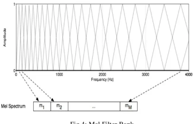
Mel(f) = 2595*log10(1 + f/700) (1) The approach to simulate the subjective spectrum is to use a filter bank, one filter for each desired mel-frequency component. The filter bank has a triangular band pass frequency response and the spacing as well as the bandwidth is determined by a constant mel-frequency interval. The mel scale filter bank is a series of 40 triangular band pass filters that have been designed to

simulate the band pass filtering believed to occur in the auditory system. This corresponds to series of band pass filters with constant bandwidth and spacing on a mel frequency scale.

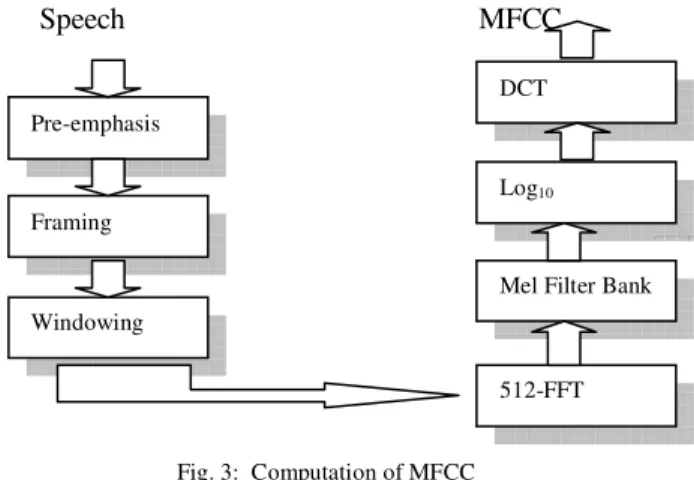
As shown in Figure 3, MFCC consists of seven computational steps. Each step has its function and mathematical approaches as discussed briefly in the following:

Speech MFCC

Fig. 3: Computation of MFCC

Pre-Emphasis processes the passing of signal through a filter which emphasizes higher frequencies. This process will increase the energy of signal at higher frequency. First order FIR filter is used, which is described in the form of difference equation as given below.

y(n)=x(n)-ax(n-1) 0 ≤ a ≤ 1 (2)

where y(n)and x(n)are the output and the input of the filter respectively. Typical value of ‘a’ is 0.95 (> 20 dB gain for high frequency).

The speech signal is divided into frames of N samples. Adjacent frames are being separated by M (M<N). Typical values used are M = 100 and N= 256. This is to ensure that the spectral properties are nearly constant and stable in the framed duration.

Each frame is passed through a window to avoid abrupt transition between the frames. Hamming window is used as window shape by considering the next block in feature extraction processing chain and integrates all the closest frequency lines. The Hamming window of length N is given as:

w(n) = 0.54 – 0.46 cos(2πn/(N-1)) 0 ≥ n ≥ N-1 = 0 otherwise (3)

As can be observed from the above equation, that the shape of the window is cosine, which ensures no ripples Feature Extraction Generate /Update Database Pre-emphasis Framing Windowing DCT Log10

Mel Filter Bank

512-FFT Feature

Extraction Similarity _Measure Decision _Logic

(3)

around the edges of the frames in frequency spectrum of the frames.

To convert each frame of N samples from time domain to frequency domain DFT is used. But complexity of DFT is N2 and Fast Fourier Transform (FFT) is N*log2(N). Hence

FFT is used to convert the time domain speech sample. In general, choose N=512, 1024 or 2m. Magnitude and phase at N equidistant digital frequencies between 0 and 2π (rad/sec). Corresponding analog frequencies are kFs/N Hz, k=0, 1... N-1.

Human hearing is not equally sensitive to all frequency bands. It is linear roughly up to 1000 Hz. It is less sensitive at higher frequencies i.e. human hearing perception is non-linear roughly above 1000 Hz. A set of filters with triangular band pass frequency response is believed to occur in the human auditory system. One filter is assigned for each desired mel-frequency component.

Fig 4: Mel Filter Bank

Human response to signal level is logarithmic. Human response is less sensitive to slight differences in amplitude at high amplitudes than low amplitudes. Logarithm compresses dynamic range of values making feature extraction less sensitive to dynamic variation. It makes frequency estimates less sensitive to slight variations in input (power variation due to speaker’s mouth moving closer to mike). Since the phase information is not useful in the recognition problem, it is discarded.

In this final step, the log mel spectrum is converted back to time. The result is called the mel frequency cepstrum coefficients (MFCC). The cepstral representation of the speech spectrum provides a good representation of the local spectral properties of the signal for the given frame analysis. Because the mel spectrum coefficients (and so their logarithm) are real numbers, coefficients are converted to time domain using the Discrete Cosine Transform (DCT).

2.2 Feature Matching

The feature vectors obtained after the first phase of the recognition are stored and used for comparison against the testing speech sample. DTW algorithm [7] is based on Dynamic Programming techniques. This algorithm is for measuring similarity between two time series which may vary in time or speed. This technique is also used to find the optimal alignment between two times series if one time series may be “warped” non-linearly by stretching or shrinking it along its time axis. This warping between two time series can then be used to find corresponding regions between the two time series or to determine the similarity between the two time series.

2.2.1 Dynamic Time Warping

The classic DTW is computed as follows:

Suppose we have two time series Q and C, of length n and m respectively, where:

Q = q1, q2… qi,…,qn (4) C = c1, c2… cj… cm (5)

To align two sequences using DTW, an n-by-m matrix where the (ith, jth) element of the matrix contains the distance d (qi, cj) between the two points qi and cj is

constructed. Then, the absolute distance between the values of two sequences is calculated using the Euclidean distance computation:

d (qi,cj) = (qi - cj)2 (6)

Each matrix element (i, j) corresponds to the alignment between the points qi and cj. Then, accumulated distance is measured by:

D (i, j) = min [D (i-1, j-1), D (i-1,j), D (i, j-1)] + d (i, j) (7) In the process of finding the optimal path, the algorithm has to follow certain constraints as listed below:

Monotonic condition: the path will not turn back on itself, both i and j indexes either stay the same or increase, they never decrease.

Continuity condition: The path advances one step at a time. Both i and j can only increase by 1 on each step along the path.

Boundary condition: the path starts at the bottom left and ends at the top right.

Adjustment window condition: a good path is unlikely to wander very far from the diagonal. The distance that the path is allowed to wander is the window length r.

Slope constraint condition: The path should not be too steep or too shallow. This prevents very short sequences matching very long ones. The condition is expressed as a

(4)

ratio n/m where m is the number of steps in the x direction and m is the number in the y direction.

After m steps in x you must make a step in y and vice versa.

3. Methodology

For the proposed work, the objective is to identify the speaker uttering as one amongst the set of speakers whose voice samples are stored in database. For this, the system is trained by speech samples of set of speakers. The speech samples of the various speakers are taken in a noise free environment and saved in database. The speech samples consist of digits ‘1’ to ‘5’. The feature vectors of the stored speech samples are evaluated. When the system is trained to identify some finite speakers, the system is tested in real time. In testing phase the speaker utters a digit. MFCC of the recorded speech is calculated and then using DTW algorithm the test sample’s feature vectors are compared against all the feature vectors stored in database. The sample whose feature vector gives least distance between the test sample, is identified as the speaker.

For the application to run successfully, the recordings for the database as well as during testing phase have to be done in noise free environment. Generally, the numbers of MFCC coefficients are around 10 to 15. For the present work, 13 coefficients are calculated.

4. Results and Discussion

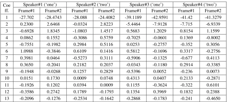
The recordings for testing purpose are done in real time and in clean environment. The table I shows the MFCC for the speech samples of four different speakers uttering two digits.

Applying DTW directly to the MFCC vectors and comparing all the speech samples of the database against the recorded one, proves to be quite time consuming. As a solution to this problem, Euclidean Distance between the feature vectors of the speech samples is found out. This facilitates faster processing and removal of majority of less probable speech samples to be applied to DTW. The first five speech samples from the database to have least Euclidean distances are selected to be applied to DTW for comparison against the test speech sample. But before evaluating Euclidean distance, the silence part from the speech samples has to be removed for reliable results. Fig. 5 shows the speech sample before and after the removal of silence period.

Fig.5: Original Signal and Silence Removed Signal

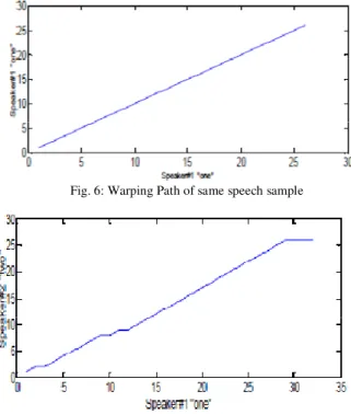
Fig.6 and Fig.7 given below show the warping paths obtained using DTW algorithm on speech samples. It is seen that the warping path between the same speech samples is a perfect straight line corresponding to least distance between the speech samples. Whereas in the second case, where the speech samples are from different speakers for different uttered word is slightly different from a straight line.

Fig. 6: Warping Path of same speech sample

(5)

Table I: MFCC coefficients for first two frames for four different speakers uttering different digits. Coe

ff.

Speaker#1 (‘one’) Speaker#2 (‘two’) Speaker#3 (‘one’) Speaker#4 (‘two’)

Frame#1 Frame#2 Frame#1 Frame#2 Frame#1 Frame#2 Frame#1 Frame#2

1 -27.702 -28.4743 -28.088 -24.4082 -39.1189 -42.9591 -41.42 -41.3279 2 0.2300 2.6468 -0.0324 2.8223 -5.4464 -7.9128 -7.715 -6.9339 3 -0.6928 1.8345 -1.0803 1.4517 0.5683 1.2029 0.8154 1.1599 4 0.0862 0.1552 -0.3086 0.5759 -0.7025 -0.0601 0.1369 -0.8002 5 -0.7551 -0.1982 0.2984 0.5116 0.0253 -0.2757 -0.352 0.3056 6 1.0988 -0.3846 0.6109 0.1416 0.5812 -0.1696 0.3317 -0.2756 7 0.3981 0.0464 -0.5273 0.3111 -0.5906 -0.1325 -0.677 0.4113 8 0.3650 -0.2041 0.2182 0.2037 -0.0343 -0.1180 0.2914 -0.3385 9 -0.1948 -0.0268 0.1257 0.2829 -0.5396 0.0052 -0.236 0.0073 10 0.0151 0.1730 0.0009 0.0748 0.4313 0.0407 0.2133 -0.2871 11 -0.1926 0.1202 0.0394 0.0009 0.1155 -0.3624 -0.322 0.6101 12 -0.3586 0.2742 0.1789 -0.1793 0.1354 0.3969 0.1832 0.2388 13 -0.2096 -0.1276 -0.2534 -0.1642 -0.2868 -0.1783 -0.241 -0.4650

The table shown below gives the difference in the distance between two speech samples using LPC and DTW. Table II: Distance between speech samples using MFCC and LPC

Speaker#1 “one” Speaker#2 “one” Speaker#3 “one” Speaker#4 “two” Speaker#5 “two” MFCC LPC MFCC LPC MFCC LPC MFCC LPC MFCC LPC Speaker#1 “one” 52.62 5.2 94.23 0.99 190.1 2.12 76.96 3.9 63.1 1.15 Speaker#2 “one” 94.23 0.99 71.43 0.58 128.1 2.25 88.22 6.45 82.19 0.72 Speaker#3 “one” 190.1 2.12 128.1 2.25 0 0 139.1 6.53 197.25 2.13 Speaker#4 “two” 76.96 3.9 88.22 6.45 203.9 6.53 79.9 4.7 60.28 5.09 Speaker#5 “two” 63.07 1.15 82.19 0.72 197.2 2.13 60.28 5.09 47.44 1.2 The recordings for testing purpose are done in real time and in

clean environment. A small experiment was conducted to compare the accuracy rate obtained for Speaker Recognition using MFCC and LPC. Both types of features were extracted from the same set of speech samples. These features were applied for comparison to DTW. The results of the experiment are tabulated. Table II shows the DTW distance between two speech samples using MFCC and LPC. From Table II it can be seen that using MFCC inter-speaker variation is higher than that using LPC. So the use of MFCC is justified.

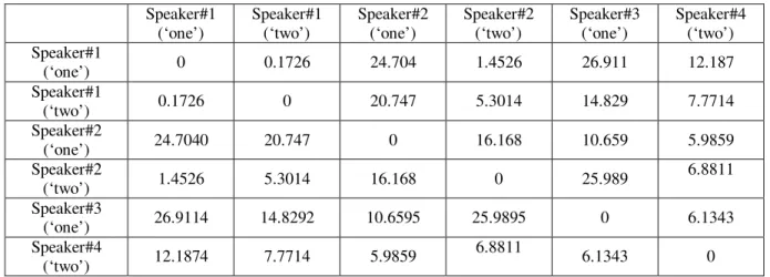
After the silence removal from the speech samples, MFCCs are evaluated for all the speech samples stored in the database. Table III shows that the DTW distance between the feature vectors of four different speakers for two different spoken

digits. It can seen that the distance between feature vectors of two different speakers uttering a word is significantly higher than that of the distance between feature vectors of same speakers.

Table IV shows the final results. The recordings are done in noise free environment. It can be seen that accuracy rates are fairly good for all the speakers. For speaker “Mandar” as it can be seen that the recognition rate is 60 % which means that during the testing phase of the project speech sample of Mandar was correctly identified 6 times out of 10 trials.

(6)

Table III: DTW distance for four different speakers uttering two different digits Speaker#1 (‘one’) Speaker#1 (‘two’) Speaker#2 (‘one’) Speaker#2 (‘two’) Speaker#3 (‘one’) Speaker#4 (‘two’) Speaker#1 (‘one’) 0 0.1726 24.704 1.4526 26.911 12.187 Speaker#1 (‘two’) 0.1726 0 20.747 5.3014 14.829 7.7714 Speaker#2 (‘one’) 24.7040 20.747 0 16.168 10.659 5.9859 Speaker#2 (‘two’) 1.4526 5.3014 16.168 0 25.989 6.8811 Speaker#3 (‘one’) 26.9114 14.8292 10.6595 25.9895 0 6.1343 Speaker#4 (‘two’) 12.1874 7.7714 5.9859 6.8811 6.1343 0

Table IV: Final Results in noise free environment

Sejal

Mandar

Bhavik

“one”

100

60

90

“two”

80

70

“three”

30

80

70

“four”

40

70

80

“five”

100

80

Fig. 8: Chart showing final results for noise free recordings Table V show the results of the system recorded in noisy environment. It can be seen from the observations of the table that the accuracy rates drop down by a small amount.

Table V: Final Results in noisy environment

Sejal

Mandar

Bhavik

“one”

90

60

80

“two”

60

70

“three”

30

70

60

“four”

40

70

80

“five”

80

70

Fig. 9: Chart showing final results for noisy environment

5. Conclusion

This paper has discussed two speaker recognition algorithms which are important in improving the speaker recognition performance. The result of the reviewed studies on Speaker Recognition yielded the answer that MFCC and DTW work well together for text-dependent Speaker Recognition purposes. The technique was able to authenticate the particular speaker based on the individual information that was included in the speech signal. Since MFCC is based on human auditory sense, the coefficients 0% 20% 40% 60% 80% 100% Sejal Mandar Bhavik 0% 20% 40% 60% 80% 100% Sejal Mandar Bhavik

(7)

provide better results compared to Linear Prediction Coefficients (LPC). The results show that these techniques could be used effectively for speaker recognition purposes. Together with smaller adjustments and improvements of the weak spots of these two techniques, it can be concluded that a fully operational Speaker Recognition program can be developed in a Matlab environment. The computational strain caused by the multi-template model used was noticeable even with only two templates using a modern computer. A speaker trained with ten repetitions of any digit would have to wait several seconds in testing mode for a result.The author hopes future evaluation of the system will determine its true performance.

References

[1] Lindasalwa Muda, Mumtaj Begam and I. Elamvazuthi, “Voice Recognition Algorithms using Mel Frequency Cepstral Coefficient (MFCC) and Dynamic Time Warping (DTW) Techniques”, Journal of Computing, Vol. 2, issue 3, March 2010, ISSN 2151-9617.

[2] Reynolds, D.A.,. "An overview of automatic speaker recognition technology,". Acoustics, Speech, and Signal Processing, 2002. Proceedings. (ICASSP '02). IEEE International Conference on , vol.4, no., pp. IV-4072-IV-4075 vol.4, 2002.

[3] Ayaz Keerio, Bhargav Kumar Mitra, Philip Birch, Rupert Young, and Chris Chatwin. "On Preprocessing of Speech Signals". International Journal of Signal Processing ; Vol.5 No.3 2009 [Page 216].

[4] PremaKanthanP. And Milkhad W.B.(2001), “ Speaker Verification/Recognition and the Importance of Selective Feature Extraction : Review”, MWSCAS Vol 1, 57-61. [5] Campbell, J. P. "Speaker Recognition",. 1999. Technical

report, Department of Defence,Fort Meade.

[6] Al-Akaidi, Marwan. "Introduction to speech processing". Fractal Speech Processing. s.l. : Cambridge University Press The Edinburgh Building, Cambridge CB2 2RU, UK, 2004.

[7] Liu, Li, He, Jialong and Palm, G.,. "Signal modeling for speaker identification,". Acoustics, Speech, and Signal Processing, 1996. ICASSP-96. Conference Proceedings., 1996 IEEE International Conference on , vol.2, no., pp.665-668 vol. 2, 7-10 May 1996.

[8] Picone, J.W.,. "Signal modeling techniques in speech recognition," . Proceedings of the IEEE , vol.81, no.9, pp.1215-1247, Sep 1993.

[9] Jayanna H S, Mahadeva Prasanna S R. "Analysis, Feature Extraction, Modeling and Testing Techniques for Speaker Recognition". IETE Tech Rev 2009;26:181-90.

[10] Md. Rashidul Hasan, Mustafa Jamil, Md. Golam Rabbani, Md. Saifur Rahman. "Speaker Identification using Mel Frequency cepstral coefficients". 3rd International Conference on Electrical & Computer Engineering ICECE 2004, 28-30 December 2004, Dhaka, Bangladesh.

[11] “Automatic Speech and Speaker Recognition, Advanced Topics”, Edited by Chin-Hui Lee, Frank K. Soong, Kuldip K.Paliwa1

[12] D. Charlet, D. Jouvet, "Optimizing Feature Set for Speaker Verification", Proceedings of the IEEE , vol.81, no.9, pp.1215-1247, 1997.

[13] Vibha Tiwari, "MFCC and its Applications in Speaker Recognition", MWSCAS Vol 1, 57-61. 2010.

[14] Md. Rashidul Hasan, Mustafa Jamil, Md. Golam Rabbani, Md. Saifur Rahman. "Speaker Identification using Mel Frequency cepstral coefficients". 3rd International Conference on Electrical & Computer Engineering ICECE 2004, 28-30 December 2004, Dhaka, Bangladesh.

[15] “Automatic Speech and Speaker Recognition, Advanced Topics”, Edited by Chin-Hui Lee, Frank K. Soong, Kuldip K.Paliwa1 International Journal of Signal Processing ; Vol.5 No.3 2009 [Page 216].

[16] Reynolds, D.A.,. "An overview of automatic speaker recognition technology,". Acoustics, Speech, and Signal Processing, 2002. Proceedings. (ICASSP '02). IEEE International Conference on , vol.4, no., pp. IV-4072-IV-4075 vol.4, 2002.

[17] Ayaz Keerio, Bhargav Kumar Mitra, Philip Birch, Rupert Young, and Chris Chatwin. "On Preprocessing of Speech Signals". International Journal of Signal Processing ; Vol.5 No.3 2009 [Page 216].

[18] Campbell, J. P. "Speaker Recognition",. 1999. Technical report, Department of Defence,Fort Meade.

[19] Archana Bhise, Sejal Shah, “ Speaker Recognition”, International Journal of Global Technology Initiatives: Vol 2 page C-123-129