Bi-label Propagation for Generic Multiple Object Tracking

(1)

Bi-label Propagation for Generic Multiple Object Tracking

Wenhan Luo

1

, Tae-Kyun Kim

1

, Bj¨orn Stenger

2

, Xiaowei Zhao

1

, Roberto Cipolla

3 1

_{Imperial College London,}

2

_{Toshiba Research Europe,}

3

_{University of Cambridge}

{w.luo12,tk.kim,x.zhao}@imperial.ac.uk, [email protected], [email protected]

Abstract

In this paper, we propose a label propagation framework to handle the multiple object tracking (MOT) problem for a generic object type (cf. pedestrian tracking). Given a tar-get object by an initial bounding box, all objects of the same type are localized together with their identities. We treat this as a problem of propagating bi-labels, i.e. a binary class label for detection and individual object labels for track-ing. To propagate the class label, we adopt clustered Multi-ple Task Learning (cMTL) while enforcing spatio-temporal consistency and show that this improves the performance when given limited training data. To track objects, we prop-agate labels from trajectories to detections based on affin-ity using appearance, motion, and context. Experiments on public and challenging new sequences show that the pro-posed method improves over the current state of the art on this task.

1. Introduction

Multiple Object Tracking (MOT) plays an important role in the computer vision literature. The problem is difficult due to frequent occlusions and appearance similarity be-tween objects. Owing to advances in object detection (es-pecially in pedestrian detection [9, 11]), in some cases the task can be solved efficiently using a tracking-as-detection approach. However, generalizing the task to other objects (see our data sets in Sec. 4) would require training a detec-tor for each new object type, which is impractical.

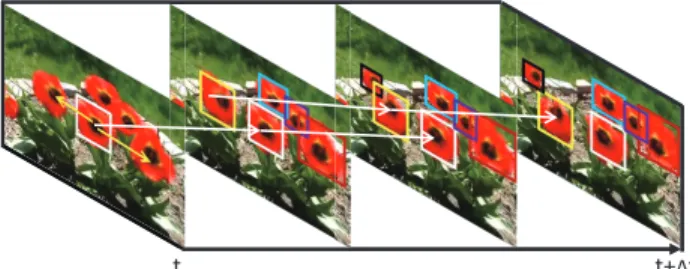
In this paper we deal with the problem of tracking mul-tiple objects of the same generic type given only one ini-tial bounding box [18], and our task is to recover multiple trajectories from image observations. Treating sliding win-dows as points in a spatio-temporal cuboid and the initial bounding box as a single labeled point, we aim to discover and track new objects by propagating labels to similar can-didates. From this perspective, our problem shares great similarity with semantic video segmentation [3] which aims to label all the pixels in a video given pixel labels in the first frame. However, these two problems have significant

dif-t t+_ѐt

Figure 1: The proposed framework. Yellow arrows indicate the propagation of class labels within the same frame and white ar-rows indicate object label propagation over time (best viewed in color).

ferences: labels in video segmentation involve only a fixed number of pre-defined classes, whereas labels in our prob-lem involve both binary classes (objectvs. background) and multiple classes (specific object identities). Thus the num-ber of classes in our problem varies as objects appear or disappear. Also, in video segmentation more than one pixel can share the same label while in our case object labels are exclusive.

We treat the labels as a combination of binary class labels and object labels (identities), and we refer to de-tection responses as an intermediate layer between image observations and trajectory estimations. Furthermore, we propose a sequential label propagation framework (Fig. 1) to propagate class labels and object labels in both spatial and temporal domains. This so calledbi-label propagation

framework coincides with a tracking-by-detection strategy: through spatially propagating the class labels (yellow ar-rows in Fig. 1), we solve the detection problem, discovering the appearance and disappearance of objects; by temporally propagating object labels (white arrows in Fig. 1), we tackle the multi-object tracking problem.

Learning a robust detector from a single training instance is challenging and standard methods tend to either overfit (e.g. using a kernel Support Vector Machine (SVM)) or un-derfit (e.g. using a linear SVM). To address the generaliza-tion issue, we train multiple detectors inspired by ensemble learning. Multiple detectors are inherently related to each other since they are dealing with the same type of objects.

(2)

The motivation of Multiple Task Learning (MTL) [10] is to learn multiple related tasks simultaneously rather than in-dependently. Thus, we treat training each of the detectors as one task and adopt clustered MTL (cMTL) [32] to reg-ularize the training process of multiple detectors. In addi-tion, we assume that images and hence detection results do not change drastically from frame to frame. We model this spatio-temporal consistency by integrating it into the cMTL formula during the class label propagation.

Our key contributions are (1) proposing a probabilistic framework for jointly propagating class and object labels in spatial and temporal domains for generic MOT and (2) in-troducing cMTL for generic object detection and improving it by considering the spatio-temporal consistency.

2. Related work

MOT methods can be grouped into two categories [23]: sequential (or online) approaches, which output trajectories on the fly, and batch (or off-line) approaches, which output results after processing all frames.

Sequential approaches derive a cost function and es-timate the lowest cost state based on sophisticated ap-pearance, motion and interaction models. For example, to maintain discrimination of individual objects, Yang et al. [29] fuse multiple components: bags of local features, a head model, and a color model of torso regions. In [6], generic object category and instance-specific information are integrated to track multiple objects in a particle filter framework. Inspired by crowd simulation models, a dy-namic model considering social motion patterns is intro-duced in [21]. Similarly, Yamaguchi et al. [27] develop an agent-based behavior model taking social and environ-mental factors into account to predict destinations of pedes-trians. The work in [14] estimates object motion based on structured crowd patterns and learns spatio-temporal varia-tions using a set of hidden Markov models.

Batch approaches exhibit a delay in outputting results, but they tend to be more robust as they can access all ob-servations simultaneously. Typical batch approaches [7, 12, 15, 28] cast the problem as a data association prob-lem, linking short-term observations such as single detec-tion responses or tracklets into longer trajectories using methods such as the Hungarian algorithm [25], greedy bi-partite matching [24], min-cost network flow [8, 26], K-Shortest Paths [4], or discrete-continuous Conditional Ran-dom Fields (CRF) [19].

Methods for generic object detection in video data re-quire either pre-trained detectors [30] or off-line train-ing [1]. Models are adapted to a given input video in order to improve the detection accuracy, e.g. by iterative boost-ing [1].

The closest work to ours is coupled detection and track-ing [16, 26]. However, most work assumes that a detector

X 1 X2 Xn Y 0 Y1 Y2 Yn Z 0 Z1 Z2 Zn (a) (b)

Figure 2: (a) Our graphical model. (b) Top to bottom: sliding windowsX, detection responsesY, and trajectoriesZ. For sake of display, we only show two trajectories (best viewed in color).

is available that has been trained off-line. For example, [26] use a dictionary of foreground images for pedestrian de-tection together with background subtraction. The work in [16] employs off-line trained pedestrian and car detec-tors. In terms of problem setting, we follow the model-free approaches in [18, 31]. The method of Zhang and van der Maaten requires initialization with bounding boxes of all objects and in contrast to our method does not discover new similar objects [31]. Luo and Kim first train a generic object detector, and subsequently employ the detector to regular-ize the training of multiple trackers [18]. In contrast to this approach, we learn detection with the help of tracking,i.e. the spatio-temporal consistency, as well as tracking based on detection, in a joint optimization framework.

3. Bi-label Propagation

3.1. Bayesian perspective

LetX,YandZrepresent sliding windows (image obser-vations), detection responses and trajectories, respectively. Fig. 2(a) shows our graphical model which has three lay-ers: image observation, detection, and trajectory layer, re-spectively. The darkly shaded nodes are observed nodes, the transparent nodes are hidden (or latent) nodes, and the lightly shaded nodes (Y0 and Z0) are partly observed as we are given only a single initial bounding box in the first frame. From the image layer to the detection response layer we propagate class labels. From the detection response layer to the trajectory layer we propagate object labels. Solving our problem corresponds to maximizingP(Z|X). Introducing variableY, we obtain

(3)

whereP(Y|X)models class label propagation (detection) andP(Z|X, Y)models object label propagation (tracking). We expand it sequentially as

max Zt,Yt

P(Zt|Xt, Yt, Z0:t₋1)P(Yt|Xt, Yt₋1), (2) and solve this estimation problem by decomposition. Tak-ing the negative logarithm of Eq. 2, we rewrite it as:

min

Wt,Θt

LC(Wt) +LO(Θt), ₍₃₎

where LC(Wt) models class label propagation, LO(Θt)

models object label propagation andWt,Θt are

parame-ters representing the detector and propagation configuration at timet. To minimize the function, we

(1) fixΘt₋1to minimizeLCviaWt;

(2) fixWt, minimizeLOviaΘt;

(3)t←t+ 1(go to the next frame).

3.2. Class label propagation

Let us review the Bayesian formula of class label propa-gationP(Yt|Xt, Yt−1)in Eq. 2. We want to maximize the likelihood ofYtconditioned on observationsXt(spatial

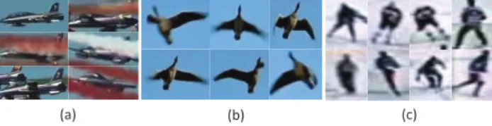
do-main) and the previous estimationYt−1(temporal domain). Our detection problem differs from the traditional detec-tion problem as we do not have sufficient data to handle large intra-class variation. Fig. 3 illustrates the extent of intra-class variation in three test videos.

As training a single classifier leads to underfitting or overfitting, we train multiple detectors and make a decision based on all of them. Moreover, by treating training each detector as one task, we investigate the relationship among multiple detectors and adopt clustered MTL to train these detectors simultaneously, improving the generalization abil-ity.

In the first frame, we add small perturbations to the ini-tial bounding box (slight shift, rotation, scale changes) to augment the positive data. Sliding windows with an over-lap (intersection/union) of the positive samples between0.2 and0.3are negative samples. In the following frames, we collect confident instances as positive samples and augment the training data in the same way.

By randomly sampling a subset of instances from the whole training data without placement m times, we ob-tainmsets of training dataXl,t,i ∈ Rd×Nt,i, i = 1, ..., m

and their labelsYt,i ∈ {1,−1}Nt,i, where the subscript “l”

means “labeled”,dis the feature space dimension andNt,i

is the number of instances. Let the multiple detectors be W = [w1, ...,wm] ∈ Rd×m. Using the least square error

the data cost term is∑m_i₌₁∥XT_l,t,iwt,i−Yt,i∥2. The

detec-tors are related as they are dealing with objects of the same type. Meanwhile, as a result of data distribution a cluster of instances are more similar to each other compared with

(a) (b) (c)

Figure 3:Illustration of intra-class variance. Shown are cropped regions from (a) theAirshowsequence, (b) theGoosesequence and (c) theHockeysequence.

others,e.g. some instances exhibit a similar viewpoint while some do not. Consequently, some detectors will be closer to each other in the model parameter space. We therefore assume that the detectors formkclusters asCj, j= 1, ..., k,

and model the coupling among all detectors following [32]:

k ∑ j=1 ∑ v∈Cj ∥wv−w¯j∥2=tr(WTW)−tr(FTWTWF), (4)

wherew¯jis the mean of the detectors within the same

clus-ter, tr(•)is the trace norm, andF ∈ Rm×k is an orthog-onal cluster indicator matrix with Fi,j = √1_n_j if i ∈ Cj

andFi,j = 0otherwise. Along with regularization of each

detector∑m_i₌₁ ∥wi∥2=tr(WTW), we have a

regulariza-tion termtr(W((1 +η)I−FFT)WT), whereηis a weight parameter. Following the convex relaxation of cMTL [32], this regularization term is relaxed totr(W(ηI+M)−1WT), subject totr(M) =k,M≼I,M∈Sm+, whereS

m

+ is the set of positive semi-definite (PSD) matrices andM≼Imeans I−Mis PSD.

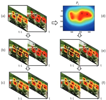
Traditional MOT applies a detector to every frame inde-pendently. By contrast, we find that detection responses in two subsequent frames should not change drastically. To utilize such information, we track confident instances via a weak tracker (KLT in our implementation) from framet−1 to framet, and produce a density mapPt(see an example in

Fig. 4(d)) by smoothing the confidence scores with a Gaus-sian (σ= 5). Based onPt, sliding windowsXu,t ∈Rd×N

(here the subscript “u” means “unlabeled”) can be weakly labeled asΨ(Pt)which is the summation of the density of

pixels close to their centers (within a circle of radius 4). The cost term∥_m1 ∑m_i₌₁XT_u,twt,i−Ψ(Pt)∥2can be

consid-ered as a weakly supervised term which propagates labels in the temporal domain. Intuitively, it assists the detector to recall more instances; Fig. 4 shows this concept. Yellow boxes indicate the detection results (also positive instances), black boxes are negative instances, and white boxes are un-labeled samples. With the help of spatio-temporal consis-tency, some candidates have weak labels indicated by the orange boxes in frame tshown in Fig. 4(e), and the weak labels help to recover missed detections, see the dashed yel-low box in frametin Fig. 4(f) which is a missed detection caused by occlusion in Fig. 4(c). Based on the terms

(4)

de-t t t t t 100 200 300 50 100 150 200 P_t (a) (b) (c) (d) (e) (f) t-1 t-1 t-1 t-1 t-1

Figure 4: Illustration of how the spatio-temporal consistency guides the detection procedure (best viewed in color).

scribed above, we have

LC(Wt) =_|α tr(Wt(ηI_{z+Mt)−1WTt_}) regularization + λ 2∥ 1 m m ∑ i=1 XT_u,twt,i−Ψ(Pt)∥2 | {z }

spatio₋temporal consistency + m ∑ i=1 1 2Nt,i∥

XT_l,t,iwt,i−Yt,i∥2

| {z }

loss

s.t. tr(Mt) =k,Mt≼I,Mt∈Sm+

(5) We treat this as a joint convex problem with regard toWand M [2]. Following [32], we adopt the Accelerated Project Gradient method to optimize this function. Labels ofXu,t

are obtained by averaging the scores of all detectors as:

Yu,t= 1 m m ∑ i=1 XT_u,twt,i (6)

We choose candidates with a score greater than zero and apply non-maximum suppression to output final class labels Yu,t∈ {−1,1}N.

3.3. Object label propagation

In the Bayesian formula Eq. 2, object label propagation isP(Zt|Xt, Yt, Z0:t₋1), where the estimation ofZtis

con-ditioned on detection responsesYtand the history of

esti-mationsZ0:t−1. Let thentrajectories at timet−1be T ={Ti|Ti=< TiA, T M i , T C i >, i= 1, ..., n}, (7) t t ȣ௧ t-1 t-1

Figure 5:Object labels are propagated from trajectories (different colors mean different objects) in framet−1to detection responses in framet. Note the proximity of a flower indicated by the black dashed circle (best viewed in color).

whereTA

i ,TiM andTiC indicate appearance, motion, and

context information, and let the m detection responses at timetbe D={Dj|Dj =< DAj, D L j, D C j >, j= 1, ..., m}, (8)

whereD_jA,DL_j andD_jCrepresent the appearance, location and context information. Tracking is carried out by propa-gating object labels from trajectories to detection responses via a configuration variableΘt ∈ Rn×m. Initially, all the

elements of Θt are 0. If an element Θtij is switched to

1, then the label of trajectoryTi is propagated to detection

response Dj, and the propagated quantity depends on the

affinityS(Ti→Dj)betweenTiandDj (here “→” means

consideringDjas a component ofTiat timet), which is

de-termined by appearance, motion and context. Fig. 5 shows this process. Objects are assumed to move smoothly, so we only consider detection responses within Ti’s

spatio-temporal proximityΩi(a circle with radiusdT h) and

mini-mize the following energy function: LO(Θt) =− ∑ i ∑ j∈Ωi S(Ti→Dj)Θtij. (9)

Appearance Model. We simply consider the intensity cue for appearance affinity. The appearance modelTA

i of

trajectoryTiconsists of the last15templates of this object,

and the appearance similarity betweenDjandTiis

SA(Ti→Dj) =med(NCC(TiA, D A

j)), (10)

where NCC(•,•)is the normalized cross-correlation (NCC) similarity measure andmed(•)is the median.

Motion Model. We maintain the past three dis-placements and predict a displacement veci weighted by [4₇,2₇,1₇], where older values are weighted higher. Given Dj, the actual displacementvecj is the difference between

DL

j and the most recent location of the object corresponding

toTi. The motion affinity is

SM(Ti→Dj) =cos(veci, vecj). (11)

Context Model. In modeling context information, we follow the work in [22] and employ 2D histograms of

(5)

T1 T2 _T 3 T4 T5 D1 D2 D3 D4 (a) (b)

Figure 6: Context model. Contexts of (a) trajectories and (b) detection responses are modeled by histograms, counting objects within an object’s proximity.

nearby objects to improve the robustness. As shown in Fig. 6, there are (a) five trajectories and (b) four detection responses. To compute a histogram forTi, we divide the

neighborhood ofTiintoMpartitions (hereM = 4for sake

of display). For each object located in this neighborhood we compute a distance vector relative toTi. According to the

distance vector, we accumulate the distance values for each partition. By normalization, we obtain anM-bin histogram Hi. The context affinity is

SC(Ti→Dj) =exp(−Bhatt(Hi,Hj)). (12)

Having obtained affinities based on three cues, we combine them as follows:

S(Ti→Dj) =SA(Ti→Dj)∗SM(Ti→Dj)∗SC(Ti→Dj).

(13) We minimize the energy (Eq. 9) by greedy search in an iterative way. First we turn off all propagation switches. We then compute the affinities of all propagation pairs and turn on the propagation switch (sayTi andDj) which most

de-creases the energy. At the same time,Dj is labeled as the

extension ofTi. We remove this pair of trajectory and

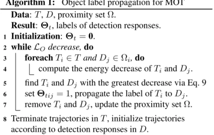
de-tection response from the search space. This procedure is repeated until there is no further energy decrease. Finally, trajectories outside the search space are updated consider-ing the extended component. The remainconsider-ing trajectories in the search space are terminated, and new trajectories are initialized based on detection responses in the search space. For clarity, the algorithm is summarized in Algorithm 1.

4. Experiments

4.1. Data sets & Setup

We test our algorithm on eight data sets, Airshow, Goose, Sailing, Zebra, Crab, Antelope, Flower1 _{and Hockey. The}

first three are new sequences obtained from YouTube videos, and the last five are public sequences [18, 20, 31]. These data sets are challenging as they contain (1) crowd

1_{This sequence is part of the original sequence in [31] (500 frames of} the original 2249 frames)

Algorithm 1: Object label propagation for MOT Data:T,D, proximity setΩ.

Result:Θt, labels of detection responses. 1 Initialization:Θt=0.

2 whileLOdecrease,do

3 foreachTi∈T andDj∈Ωi,do

4 compute the energy decrease ofTiandDj. 5 findTiandDjwith the greatest decrease via Eq. 9 6 setΘtij= 1, propagate the label ofTitoDj. 7 removeTiandDj, update the proximity setΩ. 8 Terminate trajectories inT, initialize trajectories

according to detection responses inD.

scenarios with similar objects, (2) partial or complete oc-clusions, (3) background clutter, and (4) out-of-plane rota-tions. Parametersλ,αandηin Eq. 5 are set to be0.1,0.001 and0.001respectively. The proximity parameterdT his20.

The number of detectors is 12. For each task, we sample 2₃ instances from the whole training data. We extract HoG [9], LBP and colors as features for object detection. The thresh-old to determine the confident instances is0.5. Note that for the public data sets, we refer to results reported in [18]. For data sets which are not public, we obtain results by run-ning the authors’ code ([13, 31]) or by re-implementing the method ([18] andK-SVM).

4.2. Generic object detection

We conducted experiments on generic object detection to verify the effectiveness of the proposed cMTL based detec-tion method. Five methods were compared: (1)TLD[13] which uses a detector based on Random Ferns; (2)K-SVM. We train K independent SVMs on clustered training data fromK-means clustering and detect objects by classifica-tion. This is a typical way to handle intra-class variance. The number of SVMs is four; we use the same number of clusters in our algorithm; (3)GMOT[18] is a framework which handles the same problem with a detector based on a Laplacian SVM; (4) our baseline methodBLwhich uses cMTL without the spatio-temporal consistency; (5) our full method. Table 1 shows the results. A detection response is defined as true positive if its overlap with the ground truth bounding box is at least0.5.

The results indicate that: (1)TLDonly discovers a small portion of objects on some sequences. We suspect that this is due to limitations of theTLDdetector which uses two-pixel comparisons and therefore cannot handle large intra-class variance; (2)K-SVMandGMOTshow good perfor-mance, and BLgenerally outperforms these, showing the effectiveness of cMTL to handle intra-class variance; (3) the full method outperforms all other methods; in compar-ison withBLthe recall rate is increased due to the

(6)

spatio-Table 1: Generic object detection results in terms of recall and precision values. The best results are shown in bold, the second best are underlined.

Sequence Recall Precision

TLD GMO T K-SVMBL Ours TLD GMO T K-SVMBL Ours Antelope .29 .74 .88 .77 .89 .57 .66 .71 .76 .77 Goose .66 .80 .92 .85 .94 .94 .85 .97 .98 .99 Zebra .60 .80 .66 .74 .82 .92 .97 .88 .91 .91 Crab .22 .52 .55 .56 .58 .58 .81 .70 .85 .88 Flower .21 .47 .30 .50 .63 .58 .62 .95 .94 .91 Airshow .16 .13 .38 .43 .63 .52 .56 .76 .77 .75 Sailing .60 .63 .56 .67 .84 1 .93 1 1 .99 Hockey .65 .84 .43 .65 .82 .92 .89 .75 .88 .94 Avg. .56 .56 .56 .61 .70 .67 .79 .79 .88 .89

Table 2:Comparative results for different values ofK(number of SVMs inK-SVMand, correspondingly, number of clusters in our method).

Sequence Method Recall Precision

K= 2 4 6 8 Avg. 2 4 6 8 Avg. Antelope K-SVM .90 .88 .86 .84 .87 .66 .71 .72 .73 .70 Ours .83 .89 .80 .80 .82 .81 .77 .81 .80 .80 Zebra K-SVM .66 .66 .70 .70 .68 .88 .88 .89 .87 .88 Ours .73 .82 .72 .72 .75 .85 .91 .84 .84 .86 temporal consistency.

In a separate experiment we vary the numberK in K-SVM as well as the corresponding number of clusters in our algorithm. Two representative public sequences (Anti-lope and Zebra) are used in this experiment. Table 2 shows the results, which demonstrate that our algorithm outper-forms K-SVMfor most K in terms of recall rate, which is important in our setting. Note that we keepK fixed for the other experiments; a suitable choice ofKis beyond the scope of this paper.

In a more extensive comparison of the baseline method withTLDwe obtain the precision-recall curves for the An-telope and Zebra sequences, shown in Fig. 7. BL uses a threshold on the score value to determine whether a candi-date is an object, andTLD[13] uses the percentage of ferns voting for a positive decision. The results show that our baseline method outperformsTLDconsistently.

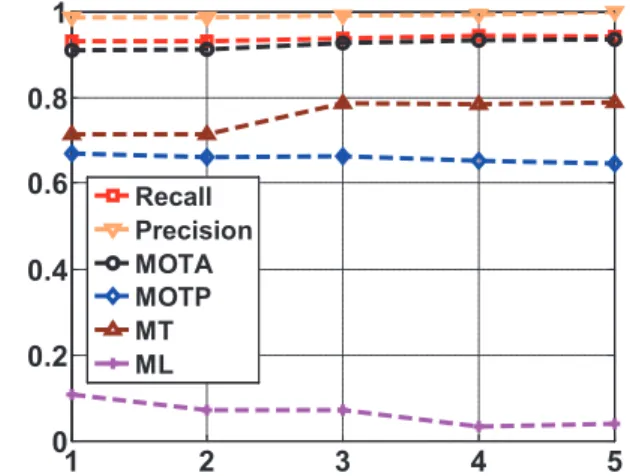
To test the variation of performance resulting from dif-ferent initial bounding boxes, we run our algorithm five times on the Goose sequence, each time labelling a differ-ent initial object. The recall rates are0.935±0.006and the precision rates 0.990±0.004, indicating low dependence on the initialization (see Fig. 8).

0 0.5 1 0.2 0.3 0.4 0.5 0.6 0.7 0.8 0.9 1 Recall Pr e c is io n Antelope BL TLD 0 0.5 1 0.65 0.7 0.75 0.8 0.85 0.9 0.95 1 Recall Pr e c is io n Zebra BL TLD

Figure 7: Precision-Recall performance ofTLDandBLon the

AntelopeandZebrasequences.

1 2 3 4 5 0 0.2 0.4 0.6 0.8 1 Recall Precision MOTA MOTP MT ML

Figure 8:Performance variation of five different initializations on theGoosesequence.

4.3. Generic MOT

We carried out experiments to compare our framework with several state-of-the-art methods on the task of detect-ing and trackdetect-ing multiple objects. The experiments are pre-sented in three parts:

(1) For each sequence we compare withTLD[13] and GMOT[18].TLDwas originally developed for single ob-ject tracking, and we extended it to multiple obob-jects by de-creasing the threshold to let it detect some similar objects and track them. It is initialized with the same bounding box as other methods.

(2) For the Zebra, Crab, Flower, Airshow and Sailing sequences, we applySPOT [31] to track multiple objects (four in our experiments) in each sequence. To compare the performance, we excerpt results corresponding to these four objects from our whole result in each sequence and evaluate the results. It is worth noting that our algorithm starts with

(7)

a single bounding box whileSPOT[31] starts with all four bounding boxes for each sequence.

(3) For the Hockey sequence, we additionally compare with [7, 6, 20] using the results from [18].

Example images are shown in Fig. 9. We adopt the cri-teria of Multiple Object Tracking Accuracy (MOTA), Mul-tiple Object Tracking Precision (MOTP) proposed in [5] as well as Mostly Tracked (MT) trajectories and Mostly Loss (ML) trajectories [17] to give quantitative results. MOTA takes the missed detection, false positives and false matches into consideration. MOTP measures the average overlap be-tween the ground truth and the true positive. MT is the ratio of the ground truth trajectories which are covered by track-ing results for more than 80% in length. ML is the ratio of the ground truth trajectories which are covered by tracking results for less than 20% in length. As shown in Table 3, the arrows following the criteria indicate the trend of better performance.

Results in Table 3 show that: (1) compared withTLD and GMOT, our method outperforms other methods on most sequences; (2) compared with SPOT, our approach achieves better results except on the MOTP metric. We sus-pect that this is due toSPOTtrackers being object-specific, thereby obtaining greater overlap scores,i.e. larger MOTP values; (3) for the Hockey sequence, our method obtains re-sults comparable with methods that use a specific off-line trained human detector.

In order to test the sensitivity on different initializations, we run our algorithm on the Goose sequence five times with different initial bounding boxes. The MOTA, MOTP, MT and ML are0.935±0.012,0.660±0.009,0.750±0.042 and0.071±0.029respectively (see Fig. 8), indicating low sensitivity to the initial labeling.

5. Conclusion

This paper proposed a framework for tracking multiple objects of the same general type, where class and object la-bels are propagated in the spatio-temporal domain. We in-troduced cMTL for generic object detection and have shown the benefit of including spatio-temporal consistency. The proposed method takes a sequential approach, entailing the limitation that object trajectories may be more fragmented than when taking a more global view of the data. Compar-ative experiments on eight sequences (five public and three new data sets) confirmed the effectiveness of the proposed method. From a practical viewpoint an advantage of our method over most other work in the area is the requirement of labeling just a single initial bounding box, thereby pro-viding a multi-object tracker without resorting to an off-line trained detector.

Table 3: Generic Multiple Object Tracking results. The table shows results in terms of four performance criteria from the lit-erature (arrows indicating direction of better performance) on five public and three new datasets.

Sequence Method MOTA↑MOTP↑MT↑ML↓

Antelope TLD [13] .088 .650 .235 .765 GMOT [18] .356 .633 .368 .368 Our method .622 .714 .691 .177 Goose TLD[13] .621 .611 .286 .179 GMOT [18] .798 .604 .643 .071 Our method .938 .649 .786 .036 Zebra TLD [13] .587 .645 .159 .420 GMOT [18] .777 .668 .435 .304 Our method .743 .683 .580 .246 SPOT [31] .661 .753 .750 0 Our method .982 .747 1 0 Crab TLD [13] .068 .646 .049 .864 GMOT [18] .391 .600 .097 .709 Our method .497 .692 .214 .689 SPOT [31] .190 .766 .500 .250 Our method .924 .724 1 0 Flower TLD [13] .053 .677 0 .632 GMOT [18] .186 .650 .053 .421 Our method .566 .718 .316 .368 SPOT [31] .372 .730 .500 .250 Our method .524 .737 .500 0 Airshow TLD [13] .013 .596 0 .733 GMOT [18] .028 .716 0 .867 Our method .415 .646 0 .067 SPOT [31] -.503 .676 0 .250 Our method .346 .650 0 0 Sailing TLD [13] .403 .737 .250 .083 GMOT [18] .548 .684 .250 .083 Our method .819 .640 .833 .083 SPOT [31] .554 .731 .750 .250 Our method .786 .652 .750 0 Hockey TLD [13] .547 .647 .179 .250 GMOT [18] .803 .691 .679 .107 Our method .766 .736 .607 .143 Brendelet al. [7] .797 .600 - -Breitensteinet al. [6] .765 .570 - -Okumaet al. [20] .678 .510 - -Avg. TLD [13] .279 .655 .140 .602 GMOT [18] .410 .637 .310 .427 Our method .613 .685 .482 .336 SPOT [31] .235 .728 .500 .200 Our method .629 .703 .650 0

References

[1] K. Ali, D. Hasler, and F. Fleuret. FlowBoost-appearance learning from sparsely annotated video. InCVPR, 2011. [2] A. Argyriou, M. Pontil, Y. Ying, and C. A. Micchelli. A

spec-tral regularization framework for multi-task structure learn-ing. InNIPS, 2007.

(8)

Zebra Antelope Crab Goose

Airshow Sailing Flower Hockey

Figure 9:Multiple object tracking results shown on frames excerpted from the videos. Different colors correspond to different objects (we only adopt 8 colors so some boxes are of the same color), the yellow lines represent trajectories.

[3] V. Badrinarayanan, F. Galasso, and R. Cipolla. Label propa-gation in video sequences. InCVPR, 2010.

[4] J. Berclaz, F. Fleuret, E. Turetken, and P. Fua. Multiple object tracking using k-shortest paths optimization. PAMI, 33(9):1806–1819, 2011.

[5] K. Bernardin and R. Stiefelhagen. Evaluating multiple object

tracking performance: the CLEAR MOT metrics.EURASIP

Journal on Image and Video Processing, 2008.

[6] M. Breitenstein, F. Reichlin, B. Leibe, E. Koller-Meier, and L. Van Gool. Robust tracking-by-detection using a detector confidence particle filter. InICCV, 2009.

[7] W. Brendel, M. Amer, and S. Todorovic. Multiobject track-ing as maximum weight independent set. InCVPR, 2011. [8] A. A. Butt and R. T. Collins. Multi-target tracking by

la-grangian relaxation to min-cost network flow. In CVPR, 2013.

[9] N. Dalal and B. Triggs. Histograms of oriented gradients for human detection. InCVPR, 2005.

[10] T. Evgeniou and M. Pontil. Regularized multi–task learning. InACM SIGKDD, 2004.

[11] P. Felzenszwalb, R. Girshick, D. McAllester, and D. Ra-manan. Object detection with discriminatively trained part-based models.PAMI, 32(9):1627–1645, 2010.

[12] J. Henriques, R. Caseiro, and J. Batista. Globally optimal solution to multi-object tracking with merged measurements. InICCV, 2011.

[13] Z. Kalal, K. Mikolajczyk, and J. Matas. Tracking-learning-detection.PAMI, 34(7):1409–1422, 2012.

[14] L. Kratz and K. Nishino. Tracking with local spatio-temporal motion patterns in extremely crowded scenes. In CVPR, 2010.

[15] C. Kuo, C. Huang, and R. Nevatia. Multi-target tracking by on-line learned discriminative appearance models. InCVPR, 2010.

[16] B. Leibe, K. Schindler, N. Cornelis, and L. Van Gool. Cou-pled object detection and tracking from static cameras and moving vehicles.PAMI, 30(10):1683–1698, 2008.

[17] Y. Li, C. Huang, and R. Nevatia. Learning to associate: HybridBoosted multi-target tracker for crowded scene. In

CVPR, 2009.

[18] W. Luo and T.-K. Kim. Generic object crowd tracking by multi-task learning. InBMVC, 2013.

[19] A. Milan, K. Schindler, and S. Roth. Detection-and

trajectory-level exclusion in multiple object tracking. In

CVPR, 2013.

[20] K. Okuma, A. Taleghani, N. de Freitas, J. Little, and D. Lowe. A boosted particle filter: Multitarget detection and tracking. InECCV, 2004.

[21] S. Pellegrini, A. Ess, K. Schindler, and L. Van Gool. You’ll never walk alone: Modeling social behavior for multi-target tracking. InICCV, 2009.

[22] V. Reilly, H. Idrees, and M. Shah. Detection and tracking of large number of targets in wide area surveillance. InECCV, 2010.

[23] X. Shi, H. Ling, X. J., and W. Hu. Multi-target tracking by rank-1 tensor approximation. InCVPR, 2013.

[24] G. Shu, A. Dehghan, O. Oreifej, E. Hand, and M. Shah. Part-based multiple-person tracking with partial occlusion han-dling. InCVPR, 2012.

[25] B. Song, T. Jeng, E. Staudt, and A. Roy-Chowdhury. A stochastic graph evolution framework for robust multi-target tracking. InECCV, 2010.

[26] Z. Wu, A. Thangali, S. Sclaroff, and M. Betke. Coupling detection and data association for multiple object tracking. InCVPR, 2012.

[27] K. Yamaguchi, A. Berg, L. Ortiz, and T. Berg. Who are you with and where are you going? InCVPR, 2011.

[28] B. Yang and R. Nevatia. An online learned CRF model for multi-target tracking. InCVPR, 2012.

[29] M. Yang, F. Lv, W. Xu, and Y. Gong. Detection driven adap-tive multi-cue integration for multiple human tracking. In

ICCV, 2009.

[30] Y. Yang, G. Shu, and M. Shah. Semi-supervised learning of feature hierarchies for object detection in a video. InCVPR, 2013.

[31] L. Zhang and L. van der Maaten. Structure preserving object tracking. InCVPR, 2013.

[32] J. Zhou, J. Chen, and J. Ye. Clustered multi-task learning via alternating structure optimization. InNIPS, 2011.