Gamma Variables
George Marsaglia
1The Florida State University
and
Wai Wan Tsang
The University of Hong Kong
Summary
The Monty Python Method for generating random variables takes a decreasing density, cuts it into three pieces, then, using area-preserving transformations, folds it into a rectangle of area 1. A random point(x;y)from that rectangle is used to
provide a variate from the given density, most of the time asx itself or a linear
function ofx. The decreasing density is usually the right half of a symmetric
density.
The Monty Python method has provided short and fast generators for normal, t and von Mises densities, requiring, on the average, from 1.5 to 1.8 uniform vari-ables. In this article, we apply the method to non-symmetric densities, particularly the important gamma densities. We lose some of the speed and simplicity of the symmetric densities, but still get a method for
variates that is simple and fast
enough to provide beta variates in the form a =( a + b ). We use an average of
less than 1.7 uniform variates to produce a gamma variate whenever1.
Imple-mentation is simpler and from three to five times as fast as a recent method reputed to be the best for changing’s.
1
Introduction
We will provide a summary of the Monty Python method here, and then show how it can be applied to provide a method for generating gamma variates for all values of the gamma parameter. The resulting algorithm is simpler and faster than any we are aware of—indeed, simple and fast enough that it can reasonably serve to provide beta variates in the form
a =(
a
+
b
). Comments on complexity and speed are in
Section 6.
The Monty Python method, developed years ago but only recently published in a journal [3], takes a decreasing sigmoid density and folds it into a rectangle of area 1, in such a way that a random point(x;y)from the rectangle can easily provide a
variate from that density—most of the time asxitself or as a linear function ofx.
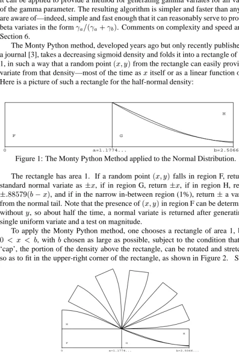
Here is a picture of such a rectangle for the half-normal density:
0 G H F a=1.1774... b=2.5066...
Figure 1: The Monty Python Method applied to the Normal Distribution. The rectangle has area 1. If a random point(x;y)falls in region F, return a
standard normal variate asx, if in region G, returnx, if in region H, return :88579(b,x), and if in the narrow in-between region (1%), returna variate
from the normal tail. Note that the presence of(x;y)in region F can be determined
withouty, so about half the time, a normal variate is returned after generating a
single uniform variate and a test on magnitude.
To apply the Monty Python method, one chooses a rectangle of area 1, base
0 < x < b, withb chosen as large as possible, subject to the condition that the
‘cap’, the portion of the density above the rectangle, can be rotated and stretched so as to fit in the upper-right corner of the rectangle, as shown in Figure 2. Since
0
F G
H H
a=1.1774... b=2.5066...
Figure 2: Rotating and stretching the cap.
‘shrink’ it vertically, so that area is preserved. And since areas of the rectangle add to 1, the slim in-between area is exactly the tail area. Packing a density into a rectangle in this way leads to relatively simple and fast procedures for generating random variables. Details and examples for normal, t, and von Mises densities are in [3].
We called this the Monty Python method because, at the time it was developed, a British TV program of that name was being shown in the US, and opening graph-ics on the program had a stylized head with its top opened and folded over with all sorts of silly images pouring out. And since our research program had investigated many different methods, we needed names to identify them. We also referred to it as the patchwork method, (see, for example, Tsang [5]), a term subsequently used by others.
2
The Monty Python method for gamma variates
In order to apply the method to generate a gamma variate
, we use the
exact-approximation method of Marsaglia [2], writing
=q(X), whereqis a monotone
function ofX, and the density ofXis such thatq(X)is exactly a
variate. That density must bef(x) =q 0 (x)q(x) ,1 e ,q(x)
=,(), and we hope to choseqsuch
thatf(x)is not necessarily close to a normal density, but rather, is close enough to
a symmetric density that we may apply the Monty Python method to it.
So our strategy is: generate a variateXfrom our nearly symmetric densityf(x)
by means of the Monty Python method, then returnq(X)as the required
variate,
for any 1. For the rare but difficult case < 1, we boost the parameter to +1by means of a method of Marsaglia that goes back to 1961: generate
as
+1 U
1=
, withU independent uniform. See Section 5.
Thisqworks remarkably well for all1: q(x)=(,1=3)(1+x= p 16) 3 ; with , p 16<x<1:
For that q, the resulting density f(x) = q 0 (x)q(x) ,1 e ,q(x) =,() is very
nearly symmetric. Furthermore, for that choice ofq(x), a single rectangle of area
1: ,3:2 < x < 3:2; 0 < y < :15625, may be used to apply the Monty Python
method, providing (total) tail areas starting at 2.5% for=1and quickly going to
less than 2%. Figure 3 showsf(x)for=1;2;4;8and the common rectangle for
applying the Monty Python method.
3
Monty Python for nearly symmetric densities,
1
.
We find we are able to apply the Monty Python method only for1. For<1
we must to resort to generating a
variate as +1 U 1= . If1is fixed and we
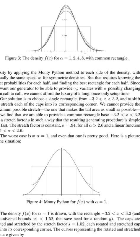
0 0.1 0.2
-4 -2 2 4
x
Figure 3: The densityf(x)for=1;2;4;8, with common rectangle.
density by applying the Monty Python method to each side of the density, with virtually the same speed as for symmetric densities. But that requires knowing the exact probabilities for each half, and finding the best rectangle for each half. Since we want our generator to be able to provide
variates with
possibly changing
from call to call, we cannot afford the luxury of a long, once-only setup time. Our solution is to choose a single rectangle, from,3:2<x <3:2, and to shift
and stretch each of the caps into its corresponding corner. We cannot provide the maximum possible stretch—the one that makes the tail area as small as possible— but we find that we are able to provide a common rectangle base,3:2<x<3:2
and a stretch factorsin such a way that the resulting generating procedure is simple
and fast. The stretch factor is constant,s=:94, for all>2:6and a linear function
for1<<2:6.
The worst case is at=1, and even that one is pretty good. Here is a picture
of the situation:
-4 -2 2 4
x
Figure 4: Monty Python forf(x)with=1.
The densityf(x)for=1is drawn, with the rectangle,3:2<x <3:2(and
the universal boundsjxj < 1:52, that save need for a randomy). The caps are
rotated and stretched by the stretch factors=1:02, each rotated and stretched cap
put into its corresponding corner. The curves representing the rotated and stretched caps are given by
Right cap:3:2(1+s),sf(s(+3:2,x)); x>0;
so that a single formula applies by attaching the sign ofxto 3.2.
If Figure 4 is enlarged enough, it becomes clear that the left cap is not quite rotated and stretched in an optimal way; there is a narrow gap that could be closed with a bettersfor the left side. But the simplicity ofs=1:02for each side in the
resulting algorithm is well worth that slight increase in tail area.
Note that for even this worst case, the probability that a variate must be returned from one of the tails is .024. This probability rapidly goes to less than .02 as
increases.
Plots off(x), the rectangle,3:2<x<3:2and the rotated and stretched caps
look much the same for>1, except that the tail areas get smaller. If we vary the
unit rectangle on which the Monty Python method is based, as a function of, we
find that we can squeeze the tail areas down to nearly 1%. But that compromises the simplicity of using a common rectangle,,3:2 < x < 3:2. We have chosen
to use that common rectangle, for which the tails are around 2%. As we shall see, providing tail variates is not a very expensive procedure.
We will describe the tail procedure in the next section. Assuming that, we may put our gamma generator, for any1, in the following simple form, with VNI,
UNI representing, resp., uniform variables from (-1,1) or (0,1) andq(x)=(, 1 3 )(1+x= p 16) 3 ,f(x)=q 0 (x)q(x) a,1 e ,q(x) =,(), ands=:94if>2:6, else:81+:84= p 16: x=3.2*VNI if |x|<1.52 return q(x) y=.15625*UNI if y < f(x) return q(x) z=s*(sign(b,x)-x) if y >.15625*(1+s)-s*f(z) return q(z) return a tail variate
Those seven lines summarize the generating procedure. Implemented directly, they provide a very concise gamma generator that is still quite fast. And it can be made very fast if quadratic pretests are inserted to avoid, most of the time, evaluation off(x)in step 4 orf(z)in step 6.
For evaluation,f takes the form
f(x)=e (3,1)ln(1+x= p 16),(, 1 3 )(1+x= p 16) 3 +c ; wherec = ln(, 1 3
)+ln(3=4),:5ln() ,ln (,(a)). The constant c
re-quires a loggamma routine unless, as we have done, one evaluates it directly to the required accuracy by means of polynomial approximations, ascis very nearly
a linear function ofwith asymptotic slope 1: c = ,1:53995,5=(36), 1=(81 2 ),1=(3240 3 ),1=(1215 4
)+. Of course, with quadratic pretests,c
is needed only if the random point(x;y)falls betweenf(x)orf(z)and its quadratic
4
Sampling from the tails.
When the random point(x;y)from the Monty Python rectangle falls into one of the
two ‘tail’ regions, we must provide anxfrom one of the two tails. But we don’t
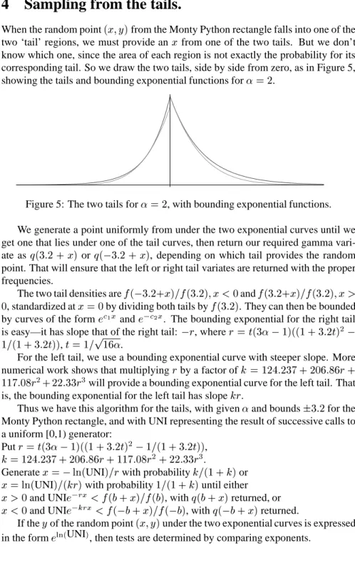
know which one, since the area of each region is not exactly the probability for its corresponding tail. So we draw the two tails, side by side from zero, as in Figure 5, showing the tails and bounding exponential functions for=2.
Figure 5: The two tails for=2, with bounding exponential functions.
We generate a point uniformly from under the two exponential curves until we get one that lies under one of the tail curves, then return our required gamma vari-ate asq(3:2+x)orq(,3:2+x), depending on which tail provides the random
point. That will ensure that the left or right tail variates are returned with the proper frequencies.
The two tail densities aref(,3:2+x)=f(3:2);x<0andf(3:2+x)=f(3:2);x> 0, standardized atx=0by dividing both tails byf(3:2). They can then be bounded
by curves of the forme c1x
ande ,c2x
. The bounding exponential for the right tail is easy—it has slope that of the right tail:,r, wherer=t(3,1)((1+3:2t)
2 ,
1=(1+3:2t)),t=1= p
16.
For the left tail, we use a bounding exponential curve with steeper slope. More numerical work shows that multiplyingrby a factor ofk=124:237+206:86r+ 117:08r
2
+22:33r 3
will provide a bounding exponential curve for the left tail. That is, the bounding exponential for the left tail has slopekr.
Thus we have this algorithm for the tails, with givenand bounds3:2for the
Monty Python rectangle, and with UNI representing the result of successive calls to a uniform [0,1) generator: Putr=t(3,1)((1+3:2t) 2 ,1=(1+3:2t)), k=124:237+206:86r+117:08r 2 +22:33r 3 .
Generatex=,ln(UNI)=rwith probabilityk=(1+k)or x=ln(UNI)=(kr)with probability1=(1+k)until either x>0and UNIe ,rx <f(b+x)=f(b), withq(b+x)returned, or x<0and UNIe ,k rx <f(,b+x)=f(,b), withq(,b+x)returned.
If theyof the random point(x;y)under the two exponential curves is expressed
in the forme ln(UNI)
5
The case
< 1.
For<1we have not found an easyq(x)for whichq 0 (x)q(x) ,1 e ,q(x) provides a family of nearly symmetric densities for the Monty Python method. So we rely on the fact that a
variate can be expressed as the product of a
+1variate and the 1=power of an independent uniform variateU:
+1 U 1= . To prove this, take logarithms. The characteristic function ofln(
+1
)is,(+1+it)=,(+1),
and the characteristic function ofln(U)=is=(+it). The product of those two
is,(+it)=,(), the characteristic function ofln(
).
6
Speed and complexity comparisons.
Many methods have been proposed for generating gamma variates. See Devroye’s thorough treatment of it and other methods for non-uniform variates [1]. We used an article by Minh [4] as an example of the current best gamma generator when we undertook to see if the Monty Python method might be better. In examining that al-gorithm, there is little doubt that the Monty Python method leads to a much simpler implementation. As for speed, we find it is also much faster. But comparisons in speed must take into account, to name a few: PC or workstation, Fortran or C, F77 or F95, Microsoft or Borland or Lahey or gnu, optimizing compilers, the way that the necessary uniform variates are provided, which parts are inline, the overhead of subroutine calls, etc.
Nonetheless, for a variety of different elements taken into account, the Monty Python method seems far and away the best we know of. For example, on a fast Silicon Graphics machine, Minh’s algorithm [4] averaged 5.234,4.324,5.572,5.473 microseconds for = 1+;2;4;10, while the Monty Python method averaged
.92,1.02,.844,.814 for those’s. Those are the times without setups. (We must use =1+for Minh, as it will not work for=1.)
The times for the MP method are based on an implementation that supplements the simple 7-line algorithm of Section 3 with quadratic pretests to avoid evaluating
f, and specific code for the tails.
Corresponding averages for repeated calls with fixed and constants
preas-signed are: 1.52, .965, .891, .846 for Minh and .64, .637, .626, .622 for Monty Python. In all comparisons, we used a common uniform generator: floatingj=69069*j
to (0,1), produced inline to avoid the overhead of an additional subroutine call. Another time comparison: on a 120 Mhz PC with Microsoft Fortran, the Minh algorithm took 29.2, 29.2, 28 microsecs for = 3;10;500, while corresponding
times for Monty Python were 9.6,9.1,9.2.
And another: on an older Sun workstation, for various, Minh averaged 75.3
microsecs, compared to 29.6 for Monty Python.
For readers who may wish to use the Monty Python method, or compare it with others, Fortran and/or C versions are available from either of us, [email protected] or [email protected].
References
[1] Devroye, Luc (1986), Non-Uniform Random Variate Generation, Springer-Verlag, New York.
[2] Marsaglia, George (1984), The exact-approximation method for generating ran-dom variables, Journal Amer. Statist. Assoc., 79, 218–221.
[3] Marsaglia, George and Tsang, Wai Wan (1997) The Monty Python Method for generating random variables, ACM Transactions on Mathematical Software, in press.
[4] Minh, Do Le (1988), Generating gamma variates, ACM Trans. on Math.
Soft-ware 14, 261–266.
[5] Tsang, Wai Wan (1982), Computer generation of random variables, Ph. D. Dis-sertation, Dept. of Computer Science, Washington State University.