A Simulation Study of Missing Data with Multiple Missing X’s

(1)

Practical Assessment, Research, and Evaluation

Volume 19 Volume 19, 2014 Article 10 2014

A Simulation Study of Missing Data with Multiple Missing X’s

Jonathan D. Rubright Ratna Nandakumar Joseph J. Gluttin

Follow this and additional works at: https://scholarworks.umass.edu/pare

Recommended Citation Recommended Citation

Rubright, Jonathan D.; Nandakumar, Ratna; and Gluttin, Joseph J. (2014) "A Simulation Study of Missing Data with Multiple Missing X’s," Practical Assessment, Research, and Evaluation: Vol. 19 , Article 10. DOI: https://doi.org/10.7275/9ew5-zd12

Available at: https://scholarworks.umass.edu/pare/vol19/iss1/10

This Article is brought to you for free and open access by ScholarWorks@UMass Amherst. It has been accepted for inclusion in Practical Assessment, Research, and Evaluation by an authorized editor of ScholarWorks@UMass Amherst. For more information, please contact [email protected].

(2)

A peer-reviewed electronic journal.

Copyright is retained by the first or sole author, who grants right of first publication to Practical Assessment, Research & Evaluation. Permission is granted to distribute this article for nonprofit, educational purposes if it is copied in its entirety and the journal is credited. PARE has the right to authorize third party reproduction of this article in print, electronic and database forms.

Volume 19, Number 10, August 2014 ISSN 1531-7714

A Simulation Study of Missing Data with Multiple Missing X’s

Jonathan D. Rubright, American Institute of Certified Public Accountants

Ratna Nandakumar, University of Delaware

Joseph J. Glutting, University of Delaware

When exploring missing data techniques in a realistic scenario, the current literature is limited: most studies only consider consequences with data missing on a single variable. This simulation study compares the relative bias of two commonly used missing data techniques when data are missing on more than one variable. Factors varied include type of missingness (MCAR, MAR), degree of missingness (10%, 25%, and 50%), and where missingness occurs (one predictor, two predictors, or two predictors with overlap). Using a real dataset, cells are systematically deleted to create various scenarios of missingness so that parameter estimates from listwise deletion and multiple imputation may be compared to the “true” estimates from the full dataset. Results suggest the multiple imputation works well, even when the imputation model itself is missing data.

Missing data are extremely common throughout social science research (Patrician, 2002; Puma, Olsen, Bell, & Price, 2009). Respondents mistakenly skip questions on a survey; pages of paper surveys get stuck together; individuals can be offended by or refuse to answer questions (Field, 2009). Regardless of reasons for missingness, all analysts at one time or another are confronted with and must address it - even if addressing it means ignoring it altogether. Yet, it is known that the missing data mechanism can impact the results of a model depending on how missingness is handled. The complexity in dealing with missingness has led some to call for statistical consultation with experts in most cases (Ferketich & Verran, 1992).

The problem is relatively simple: if respondents with missing data differ from respondents without missing data, bias can result when applying a model (Tabachnick & Fidell, 2007). However, the solutions are not so simple. Technical explications abound for missing data techniques for many types of data (Little & Rubin, 2002; Puma, et al., 2009; Schafer, 1997). However, the current literature on the use of missing data techniques is limited to exploring the impact of data missing on a single variable. Yet in practice, analysts commonly

encounter data missing on multiple variables. This article studies the impact of missingness on more than one variable when utilizing various missing data techniques.

Types of Missing Data

There are three definitions, or “types,” of missingness (Rubin, 1976). These designations are important, as the type of missingness can have a larger impact on model results than the amount of data missing from a dataset. The overall categories of missingness are missing completely at random (MCAR), missing at random (MAR), and missing not at random (MNAR).

Data are MCAR if the probability of missingness is unrelated to the value of the observation or to the value of any other variables in the data set; data are MAR if missingness depends on the value of another variable in the dataset (Allison, 2001). The final missing data pattern, MNAR, has a specified pattern, yet no secondary variable is available to explain it (Muthen & Muthen, 2004). Although some techniques are available to determine which type of missing data patterns are present (Cohen & Cohen, 1983; Cohen, Cohen, West, & Aiken, 2003), it is difficult to assess the pattern of missingness in practice (Jones, 1996).

1 Published by ScholarWorks@UMass Amherst, 2014

(3)

Practical Assessment, Research & Evaluation, Vol 19, No 10 Page 2 Rubright, Nandakumar & Glutting, Missing Data

Methods of Handling Missing Data

A number of techniques have been used to handle missing data, with success depending on the nature of the data and the nature of the missingness pattern. Common solutions historically include listwise deletion (LD), pairwise deletion, and mean substitution. Yet, more recent solutions include Maximum Likelihood, Full Information Maximum Likelihood, and Multiple Imputation (MI).

The most common way of handling missingness (and the default for all major statistical packages) is LD, which simply omits cases with missing data and runs analyses using the remaining cases. This approach works well with MCAR data, leading to unbiased parameter estimates (Allison, 2001). Still, a number of problems exist when using LD. The loss of subjects to deletion reduces power by increasing standard errors, reducing significance levels, and increasing the risk of errors of the second kind. However, when data are MAR or MNAR, LD results can be biased since the remaining cases may not be representative of the full sample (von Hippel, 2004).

In order to prevent the loss of subjects in LD, imputation techniques instead insert a reasonable value into each missing cell (Little & Rubin, 2002). The imputation technique garnering the most recent attention outside of the structural equation modeling tradition has been multiple imputation (MI). To avoid the problems of single imputations, Rubin (Rubin, 1976, 1996) developed an alternative way of including the uncertainty of imputed values by adding a portion of the residual distribution to imputed values. Rubin solves the problem of underestimating standard errors by repeating this imputation several times, generating multiple sets of new data whose imputed values vary from set to set. These separate datasets are analyzed individually, with results combined for final inferences. This process of imputing multiple times and pooling results more accurately reproduces the uncertainty surrounding the true values of missing data points.

For readers interested in implementing any of these missing data procedures, in-depth writings include Little and Rubin (2002) and Allison (2001). Additionally, Enders (2010) is a very readable book, which also helpfully provides example datasets and code for carrying out the procedures discussed here utilizing variety of statistical software programs. And, the Institute for Digital Research and Education at the University of California, Los Angeles hosts a number of

applied examples on their website at https://idre.ucla.edu/stats.

Simulation studies suggest that Maximum Likelihood and MI are generally the best methods for handling missing data (Jelicˇic´, Phelps, & Lerner, 2009). However, little data are available on how these techniques recover parameter estimates with data missing on multiple variables. This very common situation possesses a problem particularly for MI: the imputation model used to impute a value may have data missing on other variables. The extent to which MI is hampered by data missing on multiple indicators is in need of study.

Method

The purpose of this study is to compare LD and MI methods of addressing missing data on more than one variable in the context of multiple regression analysis (MRA). These techniques were selected since, other than structural equation modeling situations, they are the most widespread and commonly used missing data approaches. MRA was chosen to demonstrate the utility of these techniques because of its broad application to data in social sciences (Cohen, et al., 2003). Real data will be utilized in this study so that the impact of LD and MI on parameter estimation can be studied realistically. Various missing data conditions following MCAR and MAR are generated from real data. Parameter estimates resulting from LD and MI treatments are compared to the complete dataset results to assess bias in estimation. This procedure is replicated multiple times to reduce sampling error and to obtain estimates on how well these techniques perform on average within each condition.

Data are taken from the joint standardization sample for the Differential Ability Scales (DAS-1) and the Adjustment Scales for Children and Adolescents (ASCA) (McDermott, 1993, 1999). The dataset consists of 1,268 subjects. For this study, we utilize reading ability, spatial ability, verbal ability, and mean parental educational achievement.

In performing the MRA, spatial and verbal ability scores serve as predictors while reading scores serve as the criterion. Descriptive statistics of these variables for the complete dataset are shown in Table 1. All three variables are standardized so that regression coefficients are standardized and without an intercept. The MRA model is given as:

Reading = β1Spatial + β2Verbal + ε

2 https://scholarworks.umass.edu/pare/vol19/iss1/10

(4)

Table 1. Descriptive statistics for complete data. Variable Mean SD Minimum Maximum

Reading 100.66 14.58 55 145

Spatial 100.86 14.233 56 144

Verbal 100.2 14.35 55 140

Regression assumptions were verified for the complete data, assuring linearity, approximately normal studentized residuals, and no worrisome outliers or variance inflation factors. MRA results from the complete data are summarized in Table 2. The overall model was statistically significant, and both predictors made statistically significant, unique contributions to the prediction (p<0.001) of the criterion.

Table 2. Results of multiple regression analysis

for the complete data set

Variable B SE t ratio p value R2

Spatial 0.137 0.025 5.37 <0.001 0.349 Verbal 0.516 0.025 20.22 <0.001 Starting with this full dataset, eighteen conditions are produced with different types and percentages of missingness. Missing data are created based on three factors: the percent missing, the number of variables where missingness occurs, and type of missingness (MCAR and MAR). For the degree of missing, three levels are studied: 10% missing, 25% missing, and 50% missing. For the number of variables on which data were missing, three cases are studied: missing only on one independent variable (spatial ability), missing equally on

both variables (verbal and spatial abilities) without overlap, and missing on both variables with overlap. The combination of these two factors results in nine different combinations of data sets as displayed in Table 3.

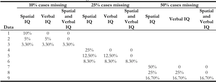
In the first three data sets 10% of data are missing. In Data 1, all 10% are missing on spatial ability. In Data 2, 5% of data are missing on spatial only, and 5% are missing on verbal only. In Data 3, one third data is missing on spatial ability, one third data is missing on verbal ability, and one third is missing on both spatial and verbal abilities. Data 4-6 and 7-9 are produced in a similar manner with 25% of cases missing and 50% of cases missing, respectively. The first nine datasets, Dataset 1 to Dataset 9, are produced as MCAR following the missing data conditions in Table 3. The next 9 datasets, Dataset 10 to Dataset 18, also following the pattern in Table 3, are produced to be MAR conditional on a related variable, mean parental educational achievement. For example, Dataset 7 has 50% data missing completely at random on the variable spatial IQ, while Dataset 16 also has 50% data missing on the variable spatial IQ, but missing conditional on the variable mean parental education. Conditional here means that subjects with lower mean parental education are more likely to have missing data.

On each of the eighteen datasets, MRA is performed using LD, and again using MI. MI is implemented utilizing 50 imputations, including the parental education variable as part of the imputation model. Regression estimates from the complete data are compared with estimates from all datasets using absolute bias. Absolute bias is computed as follows:

Table 3. Generated datasets with missing data.*

10% cases missing 25% cases missing 50% cases missing

Data Spatial IQ Verbal IQ Spatial and Verbal IQ Spatial IQ Verbal IQ Spatial and Verbal IQ Spatial IQ Verbal IQ Spatial and Verbal IQ 1 10% 0 0 2 5% 5% 0 3 3.30% 3.30% 3.30% 4 25% 0 0 5 12.50% 12.50% 0 6 8.30% 8.30% 8.30% 7 50% 0 0 8 25% 25% 0 9 16.70% 16.70% 16.70%

*Cell values denote percentage of data missing on each predictor.

3 Published by ScholarWorks@UMass Amherst, 2014

(5)

Absolute bias = complete complete     missing (1) where complete is the regression coefficient associated

with the complete data, and missing is the regression

coefficient utilizing one of the missing data techniques on one of the generated datasets. For example, suppose

complete

 = 0.5 and missing= 0.4. Then, absolute bias is

0.2 (or 20%), meaning that the bias of estimation in the regression estimate associated with the missing data technique is 20% for that condition. PROC MI and PROC MIANALYZE in SAS version 9.2 (SAS) are used to perform regression analysis and imputation, with all regression using direct-entry MRA.

Within the specifications of each condition, data are deleted randomly. However, calculations of absolute bias resulting from only one replication are subject to fluctuation due to sampling. More accurate estimates of absolute bias within each condition can be made by repeating this process multiple times. Here, the process of randomly deleting data, implementing a missing data technique, and comparing the regression estimates with those from the full dataset is repeated 500 times for each condition in order to estimate the average absolute bias within each condition.

To test overall mean differences in absolute bias across missing data techniques taking into consideration the experimental factors (percent of missingness, type of missingness, and location of missingness), a repeated measures analysis of variance (ANOVA) is carried out, one for each regression estimate [β1 (spatial) and β2

(verbal)]. Since two missing data techniques are run on a single simulated dataset, technique is treated as the repeated (within) factor. The independent variables are the amount of missingness (10%, 25%, 50%), type of missingness (MCAR, MAR), and where missingness occurs (one independent variable, two independent variables without overlap, two independent variables with overlap). The total sample size for each ANOVA is 9,000, resulting from 500 replications for each of the 18 conditions. As the focus of this work is on the missing data technique, only the within factor main effects and interactions are investigated. Between factor main effects only address average differences in absolute bias across the experimental factors, which is not of interest.

With a large number of replications (500) for each condition purposely used to be able to detect small differences, it is likely that the ANOVAs will be

over-powered. To combat the impact of an over-powered test, practical significance is determined by both a significant p-value (p<0.001) and a large effect size (partial η2_{>0.138). Partial η}2_{is the proportion of variance}

explained by the effect under scrutiny not explained by other effects in the model.

Results

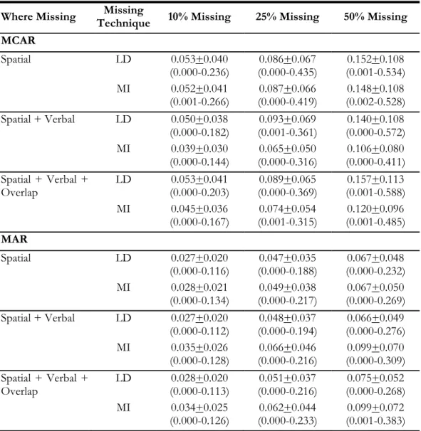
Tables 4 and 5 display results for the spatial ability coefficient and Tables 6 and 7 display results for the verbal ability coefficient. Table 4 shows means, standard deviations, and ranges of absolute bias in the spatial (β1)

coefficient by condition. It can be seen that, across all conditions, bias worsens as the percentage of missing data increases from 10 to 50 percent. Comparing results between LD and MI techniques for dealing with missing data, under the MCAR pattern for all three missing conditions bias is about the same or smaller for MI than for LD. When missing data follows the MAR pattern, however, the bias is small for MI only when data are missing on only one variable (here, spatial). When missing data occurs on more than one variable under MCAR, LD seems to be a better technique to deal with missing data.

In order to see if meaningful differences exist among the different factors studied, an ANOVA was performed to test for differences. In performing a repeated measures ANOVA on these biases, the procedure assumes that the dependent variable (mean absolute bias) is normally distributed, and that sphericity holds. Examination of the histograms and P-P plots suggests no outliers or worrisome deviation from normality. Mauchley’s Test of Sphericity is not needed, as the within factor (missing technique LD versus MI) has only two factors.

Examining the ANOVA results on the spatial biases as displayed in Table 5 shows that half of the within effects and interactions are statistically significant at p<0.001, but none meet the large effect size (partial η2_{>0.138) criteria. Since no effect meets both criteria,}

none of the effects are further explored.

The means, standard deviations, and ranges of absolute bias in the verbal (β2) coefficient by condition

are presented in Table 6. Just as in the case of spatial coefficient, across all conditions, bias worsens as the percentage of missing data increases from 10 to 50 percent. However, unlike the spatial coefficient, the bias for MI is smaller than LD for all missing conditions for both MCAR and MAR patterns. To further examine

4 https://scholarworks.umass.edu/pare/vol19/iss1/10

(6)

meaningful differences on the different factors studied, an ANOVA was performed to test for differences. The normality assumptions hold for these data as well.

Examining the ANOVA results on the spatial biases as displayed in Table 7, it can be seen that all of the within effects and interactions are statistically significant

Table 4. Mean, standard deviation, and range of bias in the spatial coefficient by

condition.

Where Missing _TechniqueMissing 10% Missing 25% Missing 50% Missing

MCAR Spatial LD 0.053+0.040 (0.000-0.236) (0.000-0.435) 0.086+0.067 (0.001-0.534) 0.152+0.108 MI 0.052+0.041 (0.001-0.266) (0.000-0.419) 0.087+0.066 (0.002-0.528) 0.148+0.108 Spatial + Verbal LD 0.050+0.038 (0.000-0.182) (0.001-0.361) 0.093+0.069 (0.000-0.572) 0.140+0.108 MI 0.039+0.030 (0.000-0.144) (0.000-0.316) 0.065+0.050 (0.000-0.411) 0.106+0.080 Spatial + Verbal + Overlap LD 0.053+0.041 (0.000-0.203) (0.000-0.369) 0.089+0.065 (0.001-0.588) 0.157+0.113 MI 0.045+0.036 (0.000-0.167) (0.001-0.315) 0.074+0.054 (0.001-0.485) 0.120+0.096 MAR Spatial LD 0.027+0.020 (0.000-0.116) (0.000-0.188) 0.047+0.035 (0.000-0.232) 0.067+0.048 MI 0.028+0.021 (0.000-0.134) (0.000-0.217) 0.049+0.038 (0.000-0.269) 0.067+0.050 Spatial + Verbal LD 0.027+0.020 (0.000-0.112) (0.000-0.194) 0.048+0.037 (0.000-0.276) 0.066+0.049 MI 0.035+0.026 (0.000-0.128) (0.000-0.216) 0.066+0.046 (0.000-0.309) 0.099+0.070 Spatial + Verbal + Overlap LD 0.028+0.020 (0.000-0.113) (0.000-0.216) 0.051+0.037 (0.000-0.268) 0.075+0.052 MI 0.034+0.025 (0.000-0.126) (0.000-0.233) 0.062+0.044 (0.001-0.383) 0.099+0.072

Table 5. ANOVA univariate testes for within effects on absolute bias of the spatial

variable. Source DF MS F p Partial _η₂ Technique 1 0.013 8.73 0.003 0.001 Technique*Percent 2 0.001 1.00 0.366 0.000 Technique*Type 1 0.809 547.29 <0.001 0.057 Technique*Percent*Type 2 0.099 66.83 <0.001 0.015 Technique*Location 2 0.004 2.73 0.065 0.001 Technique*Percent*Location 4 0.004 2.42 0.047 0.001 Technique*Type*Location 2 0.177 119.42 <0.001 0.026 Technique*Percent*Type*Location 4 0.024 15.94 <0.001 0.007 Error 8982 0.001 †p<0.001 and partial η2_>0.138 5 Published by ScholarWorks@UMass Amherst, 2014

(7)

at p<0.001. This was anticipated due to the large sample size used in the simulation. Examining the effect sizes (last column in Table 7), it can be seen that four effects meet the minimum effect size requirement. However, the main effect and two-way interactions can only be interpreted within the context of the significant three-way interaction.

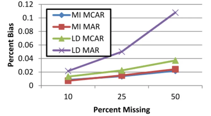
The three-way interaction between technique, percent, and type of missingness is significant,

F(2,8982)=1861.36, p<0.001, partial η2_{=0.293, Cohen’s}

large effect. A plot of the means is shown in Figure 1. As shown in Figure 1, the absolute bias in the verbal coefficient using MI is very similar with MCAR or MAR data, and gets slightly higher in bias as the percentage of missingness increases. LD performs worse than MI when handling MCAR data, and similarly increases in bias when missing data rates increase. However, LD with

MAR data shows significantly higher rates of absolute bias than MI with data MAR, and gets dramatically worse as the percentage of missingness increases.

Figure 1. Unconditional means of absolute bias in

the verbal coefficient by technique, percent, and type of missingness. 0 0.02 0.04 0.06 0.08 0.1 0.12 10 25 50 Percent Bias Percent Missing MI MCAR MI MAR LD MCAR LD MAR

Table 6. Mean, standard deviation, and range of bias in the verbal coefficient by

condition.

Where Missing _TechniqueMissing 10% Missing 25% Missing 50% Missing

MCAR Spatial LD 0.013+0.010 (0.000-0.063) (0.000-0.087) 0.023+0.017 (0.000-0.140) 0.038+0.029 MI 0.007+0.005 (0.000-0.035) (0.000-0.049) 0.011+0.008 (0.000-0.066) 0.019+0.014 Spatial + Verbal LD 0.013+0.010 (0.000-0.063) (0.000-0.079) 0.023+0.017 (0.000-0.156) 0.036+0.027 MI 0.009+0.007 (0.000-0.041) (0.000-0.058) 0.014+0.010 (0.000-0.093) 0.022+0.016 Spatial + Verbal + Overlap LD 0.014+0.010 (0.000-0.046) (0.000-0.082) 0.022+0.016 (0.000-0.165) 0.038+0.030 MI 0.010+0.008 (0.000-0.046) (0.000-0.060) 0.017+0.012 (0.000-0.113) 0.025+0.020 MAR Spatial LD 0.022+0.010 (0.000-0.050) (0.001-0.096) 0.050+0.018 (0.047-0.175) 0.107+0.025 MI 0.005+0.003 (0.000-0.021) (0.000-0.030) 0.008+0.005 (0.000-0.041) 0.011+0.007 Spatial + Verbal LD 0.022+0.010 (0.000-0.056) (0.002-0.100) 0.050+0.018 (0.021-0.171) 0.109+0.024 MI 0.008+0.006 (0.000-0.028) (0.000-0.054) 0.017+0.011 (0.000-0.102) 0.027+0.019 Spatial + Verbal + Overlap LD 0.021+0.010 (0.000-0.054) (0.002-0.115) 0.050+0.018 (0.039-0.174) 0.107+0.025 MI 0.009+0.006 (0.000-0.028) (0.000-0.063) 0.020+0.013 (0.000-0.091) 0.035+0.021 6 https://scholarworks.umass.edu/pare/vol19/iss1/10 DOI: https://doi.org/10.7275/9ew5-zd12

(8)

Discussion

This simulation study attempted to stretch the limits of missing data techniques in the novel, yet realistic, situation where data are missing on more than one X variable in the context of MRA. Previous studies have examined the impact of various missingness factors with missingness occurring on only one X variable. In this study, missingness was examined in a simulation setting where missing data were created multiple times and analyzed in terms of mean absolute bias across replications. Simulating missingness patterns multiple times allows for more accurate comparisons of absolute bias across factors of missingness type (MCAR and MAR), percent of missingness (10, 25, and 50 percent), and missing technique (MI and LD).

In this more realistic scenario, results closely mirror those from previous studies on the topic. MI preforms better at recreating the true regression coefficients than LD. Additionally, more missing data leads to more bias in the regression parameter estimates. And, MAR data is more difficult to faithfully recreate than MCAR, especially for LD.

However, these relationships only held true for one of the regression coefficients (verbal) considered in this study. As shown in Table 2, the standardized regression coefficient for the verbal variable’s prediction of reading ability was much higher than the spatial variable. Thus, there was a greater opportunity for the missing data conditions studied here to impact the estimation of that variable’s coefficient. As a limitation of this study, these results may change if a different dataset, different variables, and different relationships between variables were observed.

It is notable that the magnitude and direction of the factors considered in this study mirrored those from previous studies, since this design specifically sought to examine the impact when data were missing on more than one variable. Interestingly, the location of missingness did not impact the amount of bias in the regression coefficients. That is, it did not matter in this case whether data were missing on one variable, on two variables, or on two variables with overlap. This is especially important since the MI method requires the specification of an imputation model that depends on these supplementary variables to guide the imputation. These results reaffirm that MI works better than LD, especially when data are MAR. This study also provides confidence that MI can perform in cases where data are missing on multiple variables, even when the imputation model itself is missing data.

References

Allison, P. (2001). Missing data. Thousand Oaks, CA: Sage Publications.

Cohen, J., & Cohen, P. (1983). Applied multiple regression/correlation analysis for the behavioral sciences

(Second ed.). Hillsdale, NJ: Erlbaum.

Cohen, J., Cohen, P., West, S., & Aiken, L. (2003).

Applied multiple regression/correlation analysis for the behavioral sciences (Third ed.). Mahwah, NJ: Erlbaum.

Enders, C. K. (2010). Applied missing data analysis. New York: Guilford Press.

Ferketich, S., & Verran, J. (1992). Analysis issues in outcomes research Patient outcomes research: Examining the effectiveness of nursing practice (pp. 174-188). Washington, DC: U.S. Department of Health

Table 7. ANOVA univariate tests for within effects on absolute bias of the verbal

variable. Source DF MS F p Partial _η₂ Technique 1 3.268 17507.3 <0.001 0.661† Technique*Percent 2 0.626 3350.96 <0.001 0.427† Technique*Type 1 1.367 7322.33 <0.001 0.449† Technique*Percent*Type 2 0.347 1861.36 <0.001 0.293† Technique*Location 2 0.035 189.68 <0.001 0.041 Technique*Percent*Location 4 0.004 21.02 <0.001 0.009 Technique*Type*Location 2 0.008 40.34 <0.001 0.009 Technique*Percent*Type*Location 4 0.003 14.34 <0.001 0.006 Error 8982 0.000 †p<0.001 and partial η2_>0.138. 7 Published by ScholarWorks@UMass Amherst, 2014

(9)

and Human Services.

Field, A. (2009). Discovering Statistics Using SPSS (Third ed.). Thousand Oaks, CA: Sage.

Jelicˇic´, H., Phelps, E., & Lerner, R. (2009). Use of missing data methods in longitudinal studies: The persistence of bad practices in developmental psychology. Developmental Psychology, 45, 1195-1199. Jones, M. (1996). Indicator and stratification methods

for missing explanatory variables in multiple linear regression. Journal of the American Statistical

Association, 91, 222–230.

Little, J., & Rubin, D. (2002). Statistical analysis with missing data (Second ed.). New York: Wiley. McDermott, P. (1993). National standardization of

uniform multisituational measures of child and adolescent behavior pathology. Psychological Assessment, 5, 413-424.

McDermott, P. (1999). National scales of differential learning behavior among American children and adolescents. School Psychology Review, 28, 280-291. Muthen, L., & Muthen, B. (2004). Mplus user guide. Los

Angeles: Statmodel.

Patrician, P. (2002). Multiple Imputation for Missing Data. Research in Nursing & Health, 25, 76-84. Puma, M., Olsen, R., Bell, S., & Price, C. (2009). What

to do when data are missing in group randomized controlled trials (NCEE 2009-0049). Washington, DC:

National Center for Education Evaluation and Regional Assistance, Institute of Education Sciences, U.S. Department of Education. Rubin, D. (1976). Inference and missing data.

Biometrika, 63, 581-592.

Rubin, D. (1996). Multiple imputation after 18+ years.

Journal of the American Statistical Association, 91, 473-489.

SAS (Version 9.2). Cary, NC: SAS Institute Inc. Schafer, J. (1997). Analysis of incomplete multivariate data.

London: Chapman & Hall.

Tabachnick, B., & Fidell, L. (2007). Using multivariate statistics (Fifth ed.). Boston: Allyn and Bacon. von Hippel, P. T. (2004). Biases in SPSS 12.0 missing

value analysis. American Statistician, 58, 160–165.

Citation:

Rubright, Jonathan D, Nandakumar, Ratna and Gluttin, Joseph J. (2014). A Simulation Study of Missing Data with Multiple Missing X’s. Practical Assessment, Research & Evaluation, 19(10). Available online: http://pareonline.net/getvn.asp?v=19&n=10

Authors:

Jonathan D Rubright (corresponding author) American Institute of Certified Public Accountants Psychometrician, Examinations Team

Princeton South Corporate Center 100 Princeton South, Suite 200 Ewing, NJ 08628

Jrubright [at] aicpa.org

Ratna Nandakumar University of Delaware School of Education 113 Willard Hall Newark, DE 19716 Joseph J. Glutting University of Delaware School of Education 113 Willard Hall Newark, DE 19716 8 https://scholarworks.umass.edu/pare/vol19/iss1/10 DOI: https://doi.org/10.7275/9ew5-zd12