Approximate Bayesian techniques for inference in stochastic dynamical systems

inference in stochastic dynamical

systems

M

D. V

– A

U

–

September 2010

This copy of the thesis has been supplied on condition that anyone who consults it is un-derstood to recognise that its copyright rests with its author and that no quotation from the thesis and no information derived from it may be published without proper acknowl-edgement.

Approximate Bayesian techniques for inference

in stochastic dynamical systems

M

D. V

Doctor of Philosophy, 2010

Thesis Summary

This thesis is concerned with approximate inference in dynamical systems, from a variational Bayesian perspective. When modelling real world dynamical systems, stochastic differential equa-tions appear as a natural choice, mainly because of their ability to model the noise of the system by adding a variant of some stochastic process to the deterministic dynamics. Hence, inference in such processes has drawn much attention. Here two new extended frameworks are derived and presented that are based on basis function expansions and local polynomial approximations of a recently proposed variational Bayesian algorithm. It is shown that the new extensions converge to the original variational algorithm and can be used for state estimation (smoothing). However, the main focus is on estimating the (hyper-) parameters of these systems (i.e. drift parameters and diffusion coefficients). The new methods are numerically validated on a range of different sys-tems which vary in dimensionality and non-linearity. These are the Ornstein-Uhlenbeck process, for which the exact likelihood can be computed analytically, the univariate and highly non-linear, stochastic double well and the multivariate chaotic stochastic Lorenz ’63 (3-dimensional model). The algorithms are also applied to the 40 dimensional stochastic Lorenz ’96 system. In this inves-tigation these new approaches are compared with a variety of other well known methods such as the ensemble Kalman filter / smoother, a hybrid Monte Carlo sampler, the dual unscented Kalman filter (for jointly estimating the systems states and model parameters) and full weak-constraint 4D-Var. Empirical analysis of their asymptotic behaviour as a function of observation density or length of time window increases is provided.

Keywords: Bayesian inference, variational techniques, dynamical systems, stochastic

1 Introduction 13

1.1 How random are phenomena? . . . 14

1.2 From ODEs to SDEs . . . 15

1.3 Bayesian inference . . . 18

1.4 Thesis outline . . . 19

1.5 Disclaimer . . . 20

2 Problem statement and existing methodologies 22 2.1 Foreword . . . 23

2.1.1 Chapter outline . . . 23

2.2 Stochastic processes . . . 23

2.2.1 Examples . . . 24

2.3 Partially observed diffusions . . . 26

2.4 Problem definition . . . 27 2.5 Existing methodologies . . . 28 2.5.1 Sequential approaches . . . 28 2.5.2 MCMC approaches . . . 29 2.5.3 Variational approaches . . . 30 2.5.4 Non-Bayesian approaches . . . 31 2.6 Discussion . . . 33 3 Systems studied 34 3.1 Foreword . . . 35 3.1.1 Chapter outline . . . 35

3.2 The Ornstein-Uhlenbeck process . . . 35

3.3 The double well system . . . 38

3.4 The Lorenz ’63 (3D model) . . . 39

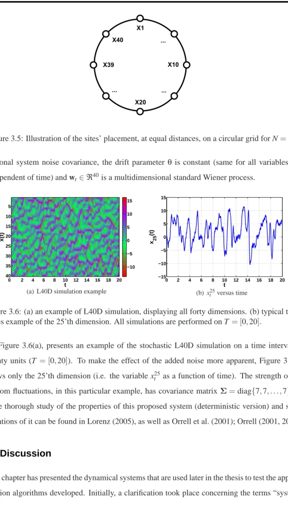
3.5 The Lorenz ’96 (40D model) . . . 40

3.6 Discussion . . . 42

4 The variational Gaussian process approximation algorithm 44 4.1 Foreword . . . 45

4.1.1 Chapter outline . . . 45

4.2 Basic setting . . . 46

4.3 Approximate inference for diffusions . . . 46

4.3.1 Variational Free energy . . . 47

4.3.2 Optimal approximate posterior process . . . 47

4.3.3 Gaussian process posterior moments . . . 48

4.4 State estimation (smoothing algorithm) . . . 48

4.5 Hyper-parameter estimation . . . 50

4.5.1 Discrete approximations to the posterior distributions . . . 51

4.5.3 Parameters to estimate . . . 53

4.6 Discussion . . . 54

5 Radial basis function extension 55 5.1 Foreword . . . 56

5.1.1 Chapter outline . . . 56

5.2 Radial basis function networks . . . 56

5.3 Global approximation of the variational parameters . . . 57

5.4 Results of state estimation . . . 60

5.5 Results of parameter estimation . . . 66

5.6 Discussion . . . 72

6 Local polynomial extension 74 6.1 Foreword . . . 75

6.1.1 Chapter outline . . . 75

6.2 Polynomial approximation of the variational parameters . . . 75

6.3 Numerical simulations . . . 80

6.3.1 Experimental setup . . . 80

6.3.2 Results of state estimation . . . 81

6.3.3 Results of parameter estimation . . . 87

6.3.4 Stochastic Lorenz ’96 (40D) . . . 91

6.4 Discussion . . . 93

7 Comparison with other methods 95 7.1 Foreword . . . 96

7.1.1 Chapter outline . . . 96

7.2 Methods implemented . . . 97

7.2.1 Ensemble Kalman filter / smoother . . . 97

7.2.2 Unscented Kalman filter / smoother / dual estimation . . . 98

7.2.3 Hybrid Monte Carlo . . . 100

7.2.4 Full weak constraint 4D-Var . . . 101

7.3 State estimation . . . 104

7.4 Parameter estimation . . . 107

7.4.1 Infill asymptotic behaviour . . . 107

7.4.2 Increasing domain asymptotic behaviour . . . 112

7.5 Discussion . . . 115 8 Conclusions 118 8.1 Foreword . . . 119 8.2 Summary . . . 119 8.3 Future directions . . . 122 8.4 Epilogue . . . 125

A Derivations of the VGPA framework 133 A.1 Basic setting . . . 133

A.2 Approximate Inference . . . 134

A.2.1 Optimal approximate posterior process . . . 136

A.2.2 Smoothing algorithm . . . 139

A.3 Parameter Estimation . . . 148

A.3.1 Initial State . . . 148

A.3.2 Drift Parameter . . . 150

A.3.3 System Noise Covariance Parameter . . . 150

A.4 Summary . . . 152

B Computing the new gradients of the RBF extension 153 B.1 Gradient of the approximate

L

B.2 Gradient of the approximate

L

C Computing the new gradients of the LP extension 155 C.1 Gradient of the approximate

L

C.2 Gradient of the approximate

L

D Analytic expressions of the systems studied 157 D.1 Ornstein - Uhlenbeck (OU) system equations . . . 157

D.2 Double Well (DW) system equations . . . 162

D.3 Lorenz ’63 (L3D) system equations . . . 167

D.4 Approximations using the unscented transformation . . . 176

E Approximate solutions of the moment equations 180 E.1 Marginal means . . . 181

E.2 Marginal variances . . . 183

1.1 An example of ODE vs SDE . . . 17

1.2 Probabilities from a frequency point of view . . . 18

2.1 Examples of standard Wiener process in 1D and 2D. . . 26

3.1 Example of an OU trajectory . . . 37

3.2 The double well potential & simulations . . . 38

3.3 Chaotic behaviour of Lorenz ’63 dynamical system. . . 39

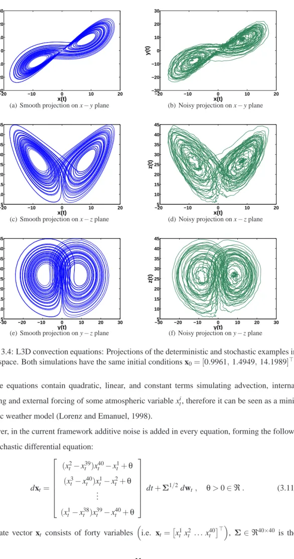
3.4 L3D convection equations: Projections in phase space. . . 41

3.5 L40D latitude circle . . . 42

3.6 Lorenz ’96 simulation example . . . 42

5.1 An example of a radial basis function network . . . 57

5.2 Assumed “true” trajectories of the non-linear systems, for the validation of the RBF approximation framework . . . 61

5.3 HMC vs RBF approximation, on the DW system . . . 62

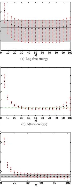
5.4 Comparison of the log free energy and the KL divergence, at convergence . . . . 64

5.5 Sensitivity of the RBF approximation to the widths of the Gaussian basis functions 65 5.6 HMC vs RBF approximation, on the L3D system . . . 66

5.7 Summary statistics illustrating the convergence of the RBF approximation to the original VGPA on the L3D . . . 67

5.8 Results on the stochastic L40D . . . 67

5.9 Approximate marginal likelihood profiles for the DW (hyper-) parameters . . . . 68

5.10 Conditional estimation of the DW (hyper-) parameters . . . 69

5.11 Joint estimation ofσ2andθ, for the DW system . . . 69

5.12 L3D𝜽andΣ_{profiles . . . . 70}

5.13 Summary statistics for the SCG number of iterations . . . 71

5.14 L40D (hyper-) parameter profiles . . . 71

6.1 An example of the local polynomial approximation, on a univariate system . . . 76

6.2 Different approximation methods on At and bt . . . 79

6.3 Runge-Kouta 2’nd order integration method, with the LP approximation algorithm 80 6.4 OU and DW sample paths used for the validation of the LP algorithm . . . 81

6.5 L3D example used for the validation of the LP algorithm . . . 81

6.6 Marginal mt and st of the LP approximation on the OU system . . . 82

6.7 Summary statistics of the LP convergence to the original VGPA, on the OU system 83 6.8 HMC vs LP on a single DW realisation . . . 84

6.9 Summary statistics of the LP convergence to the original VGPA, on the DW system 84 6.10 Free energy (LP algorithm) as both order of polynomials (Mo) and number of observations (Nobs) vary . . . . 85

6.11 HMC vs LP on a single L3D realisation . . . 86 6.12 Potential energy trace of the HMC posterior sampling algorithm, on the L3D system 86

6.13 Summary statistics of the LP convergence to the original VGPA, on the L3D system 87 6.14 OU system: profile marginal likelihood and discrete approximation to the posterior

distribution of the drift parameter, obtained with the LP algorithm . . . 88

6.15 OU system: profile marginal likelihood and discrete approximation to the posterior distribution of the noise parameter, obtained with the LP algorithm . . . 89

6.16 DW system: profile marginal likelihood and discrete approximation to the poste-rior distribution of the drift parameter, obtained with the LP algorithm . . . 90

6.17 DW system: profile marginal likelihood and discrete approximation to the poste-rior distribution of the noise parameter, obtained with the LP algorithm . . . 90

6.18 L3D system: profile marginal likelihood of the drift parameter vector𝜽 and the diagonal elements of the system noise matrixΣ_{, obtained with the LP algorithm . 91} 6.19 L3D system: approximations to the posterior distribution of the drift parameter vector𝜽, obtained with HMC sampling and the LP algorithm . . . 92

6.20 Lorenz 40D: original sample path and assimilation examples with the LP algorithm 92 6.21 Lorenz 40D: approximate marginal profiles for the drift parameterθand the sys-tem noise variance on the 20’th dimension. . . 93

7.1 Ensemble Kalman filter . . . 97

7.2 Ensemble Kalman filter and smoother . . . 105

7.3 Unscented Kalman filter and smoother . . . 105

7.4 Gaussian process regression with the squared exponential and OU kernels . . . . 105

7.5 Variational Bayesian vs MCMC solution . . . 106

7.6 Mapping the results of the dual UnKF algorithm to a single point estimate (mean value) . . . 108

7.7 Estimation of the drift parameters in the OU and DW systems, for the increasing observation density case . . . 108

7.8 Estimation of the noise parameters in the OU and DW systems, for the increasing observation density case . . . 109

7.9 Joint estimation of the drift and noise parameters in the OU and DW systems, for the increasing observation density case . . . 110

7.10 Infill asymptotic estimation results for the L3D drift parameter vector𝜽 . . . 111

7.11 Infill asymptotic estimation results for the L3D noise diagonal elements ofΣ _{. . 111}

7.12 Estimating jointly the drift and noise parameters of the L3D system with increasing observation density . . . 112

7.13 Example of an extended time-window used for the increasing domain asymptotics 113 7.14 Estimation of the drift parameterθof the OU and DW systems, in the increasing domain case . . . 114

7.15 Estimation of the noise parameterσ2_{of the OU and DW systems, in the increasing} domain case . . . 114

7.16 Jointly estimated drift and noise parameters of the OU and DW systems, in the increasing domain case . . . 115

7.17 Increasing domain asymptotic results, when estimating the L3D drift parameter vector𝜽 . . . 115

7.18 Increasing domain asymptotic results, when estimating the L3D diagonal noise parameters ofΣ _{. . . . 116}

7.19 Estimating jointly the drift parametersσ,ρandβ, and the system noise coefficients σ2 x,σ2y andσ2z, of the L3D system . . . . 116

3.1 Summary of dynamical systems. . . 43

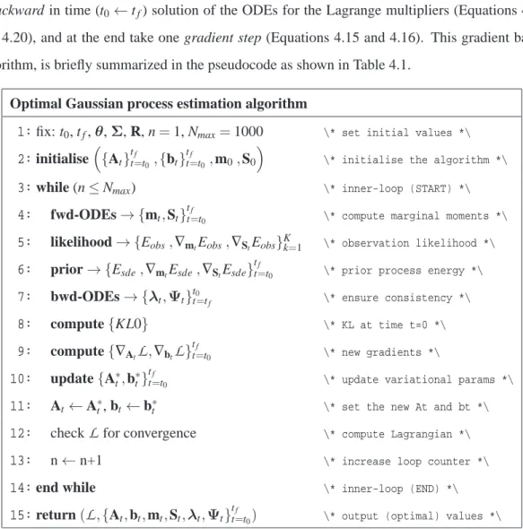
4.1 Pseudocode of the optimal Gaussian process approximation (state estimation) . . 50

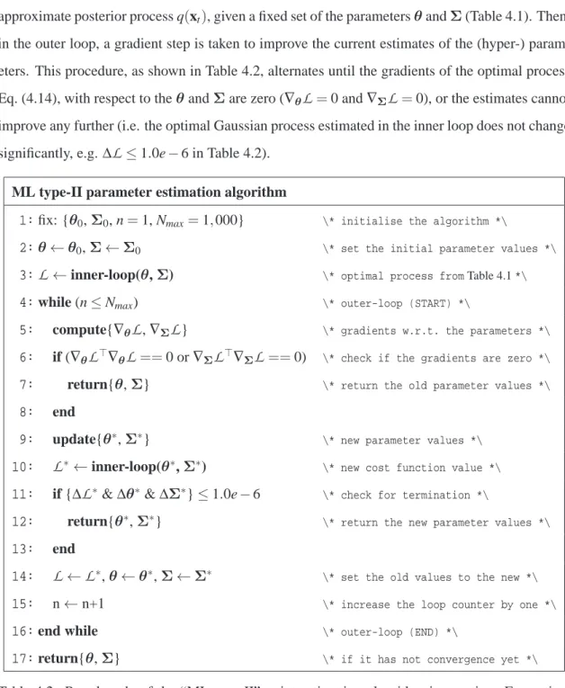
4.2 Pseudocode of the “ML type-II” point estimation algorithm . . . 52

5.1 Example ofΦ_{(t)matrix . . . . 59}

5.2 Experimental setup for the RBF framework . . . 60

6.1 Example ofΠj_{(t)matrix . . . . 78}

Undoubtedly, the person to whom I owe the most in completing this PhD thesis is my supervisor Dan Cornford. First, for giving me the opportunity to pursue one of my dreams, by offering me this PhD position and second because throughout all these four years he was very supportive, inspiring and helpful.

I am particularly thankful to professor Manfred Opper which as part of the variational in-ference in stochastic dynamic environmental models (VISDEM) project, helped me the most in understanding the variational methodology as described in Chapter 4 in this thesis. I also feel very privileged for giving me the opportunity (twice) to visit him in Berlin and work together on different extensions of the proposed variational algorithm. Also special thanks deserve Cedric Archambeau, Yuan Shen and the rest of the VISDEM project team.

An important factor that is often neglected when someone is looking back in time to resume his path is the environment in which that path was taken. I can proudly say that I was a mem-ber of the Non-linearity and Complexity Research Group (NCRG)1 at Aston University. During the first three months of my PhD the pattern analysis and neural networks (PANN) courses, that I had to undertake as part of my training, was a true “crash test” and proved an invaluable tool for the rest of my PhD. I also want to grasp the opportunity and say a big thank you to all mem-bers of the NCRG for exchanging ideas and providing insightful comments on various occasions through individual talks and group seminars. In addition I want to thank Vicky Bond for all the administrative assistance that she provided, relieving all the bureaucratic burden.

However a PhD life is not only studying and doing research. For the moments outside the lab I thank in particular my friends Erik Casagrande, Jack Raymond, Remi Barillec, Alexis Boukou-valas, George Lychnos and Patrick McGuire. Special thanks to Erik, Jack and George for being also my flatmates for almost three years.

My PhD was funded for three years from the Engineering and Physical Sciences Research Council (EPSRC), via the VISDEM project, and partially from other sources found by my super-visor. That helped critically in maintaining my focus and energy in doing my research.

Last but not least I want to express my sincere gratitude to my professors from Alexander Tech-nological Educational Institute of Thessaloniki in Greece, Panagiotis Adamidis and Konstantinos Katopodis who encouraged me and supported me in the beginning of my research career.

The need for a unified notation in the field of data assimilation has been well established (Ide et al., 1997). In order to assist the reader with the mathematical notation and glossary, used throughout this thesis, the following tables summarize the most commonly found symbols and expressions. Each term will be defined properly, when first appeared and further definitions and clarifications will be provided when necessary. As a general rule bold fonts are used for vectors or matrices, while normal fonts for scalars. Lower-case Latin letters will denote scalars or vectors, whilst upper-case matrices. Greek letters will denote model parameters.

For better presentation the notation has been organised in tables. First are given some com-monly found mathematical symbols.

Mathematical symbols and expressions Description

∼ is distributed as

∝ is proportional to

≈ approximately equal

∂a partial derivative with respect to scalar a

∇a gradient with respect to vector a

ln natural logarithm

O

pdf probability density function

w.r.t. with respect to

Next are considered the sets of numbers. In this thesis the most frequently used set is the one of real numbers. However, the set of natural numbers is used when indexing the elements of vectors or matrices, with the asterisk symbol (_∗) denoting exclusion of the zero number.

Sets Description

ℜ set of real numbers

N(∗) set of natural numbers (* excluding zero) ℜD _{D-dimensional set of real numbers}

To avoid confusion the vectors are considered column-wise unless transposed. When a vector has no index is assumed to be a (continuous) random variable. The most common index is ’t’ and denotes (continuous) time dependence (e.g. the state vector xt). For discrete time dependence the

index ’k’ is more favourable.

Vectors Description

x_∈ℜD real valued column vector

xi∈ℜ i’th element of the vector x xt∈ℜD (continuous) time dependent state vector xk∈ℜD (discrete) time dependent state vector, i.e. xk=xt=tk yk∈ℜD (discrete) time dependent observation vector

Matrices follow as a natural extension of vectors. Only upper-case letters are used and unless otherwise stated they are considered square (D_×D), where ’D’ is the number of rows /columns. If every element of a matrix is time dependent, then for notational convenience this dependency will be denoted as subscript on the whole matrix rather than on each individual element (see Appendix D).

Matrices Description

K_∈ℜD×D real valued matrix

Krc∈ℜ r’th row c’th column scalar element of K K⊤ transposed matrix

K−1 inverted matrix tr_{K_} trace of matrix

∣K_∣ determinant of matrix diag(K) diagonal elements of matrix K

I_∈ℜD×D Identity matrix

To identify a specific class of distribution, calligraphic capital letters are used, such as

N

G

Distributions Description

N

G

G

p(x) true marginal distribution

q(x) approximate marginal distribution

p(y_∣x) conditional distribution of y given x

p(y,x) joint distribution of y and x

p(x0:N) shorthand notation of p(x0,x1, . . . ,xN)

Some special notation that is used to describe the variational framework in Chapter (4) is given in the following table. Proper definitions of the vectors, matrices and functions are also given in the same section.

Special notation Description

f(xt)∈ℜD drift function

gL(xt)∈ℜD (linear) approximation function

𝜽_∈ℜD _{drift parameter vector} wt ∈ℜD Wiener process

Σ_∈ℜD×D _{system noise covariance matrix}

R_∈ℜD×D measurement error covariance matrix

H_∈ℜD×D (linear) observation operator

E_{x_}q(x) expectation of x w.r.t. q(x)

1

Introduction

CONTENTS

1.1 How random are phenomena? . . . . 14

1.2 From ODEs to SDEs . . . . 15

1.3 Bayesian inference . . . . 18

1.4 Thesis outline . . . . 19

“I cannot believe that God plays dice with the cosmos.” — Albert Einstein, German physicist. “Consideration of black holes suggests, not only that God does play dice, but

that he sometimes confuses us by throwing them where they can’t be seen.”

— Stephen W. Hawking, British physicist.

1.1

How random are phenomena?

One of the main characteristics that distinguish the human species from the rest of the species on this planet is its intrinsic curiosity to better understand the world that surrounds them. Unlike the other animals, humans are not content to satisfy only their basic needs and instincts, like thirst, hunger, self-preservation, breeding, etc. What is more interesting, is the human ability to create questions that themselves, cannot answer.

In the early beginnings of civilisation, humans were faced with a lot of queries concerning mostly the natural phenomena. The answer, at that time, was simple; for everything was respon-sible a “God”. A God was raising the sun every morning and took it back in the night, another God was responsible for bringing rain, someone else was the one “punishing” humans with natu-ral disasters, when they were misbehaving and so on1. However, the advanced ability of humans (compared to the other animals) to observe and draw conclusions helped in finding patterns and creating physical “laws” that describe the observed phenomena. Ultimately the goal of science is to understand how things work and if possible to make predictions about them (Orrell, 2007).

Pierre Simon Laplace, the famous French mathematician and physicist, laid the foundations of deterministic science. He believed that there exists a set of well defined equations that predict ev-erything in the universe (even human behaviour) given an accurate initial condition of the system; i.e. if it was possible to specify the exact position and momentum of every particle, at a single time instant, then the evolution of the universe could be uniquely determined.

The scientific belief that the whole cosmos is completely and uniquely determined by a set of equations that describe everything was very strong, until the beginning of the 20’th century, when the work of two German physicists, Max Planck with the quantum principle (early 1900) and Werner Heisenberg with the uncertainty principle (1926), laid the foundations of what is known today as Quantum Theory or Quantum Mechanics. The uncertainty principle, roughly states that the more accurately the position of a particle is measured, the greater the uncertainty in its mo-mentum and vice versa. Therefore, even if Laplace’s belief was right and a single mathematical equation, given an infinitesimally accurate initial condition can predict everything, then the

uncer-tainty principle, if accepted, makes sure that this cannot happen because we would never be able

to measure the initial conditions infinitesimally accurate. Therefore, nature itself limits human curiosity to perform predictions.

Even though quantum mechanics imply that matter is by definition indeterministic and can be described only in a probabilistic way, someone can argue that what appears random to us is because we are still unable to understand the underlying dynamics that pushes the electron from one quantum state to the other. Albert Einstein, one of the most recognized scientists of the past century, contributed a lot to the development of quantum theory (in fact he was awarded a Nobel prize), but was a deeply religious person and refused to accept that randomness exists in the universe and believed, until the very end of his life, that the universe operates under complete Law

and Order.

Nevertheless, there is room for both scientific beliefs (deterministic and random) to co-exist. Even though quantum phenomena are mostly observed in microscopic level when averaging over a huge number of particles, phenomena can still be adequately described by deterministic laws. After all, following Ockhams’ Razor: “a theory should be no more complicated than necessary”.

1.2

From ODEs to SDEs

Consider a system whose macroscopic behaviour (i.e. state of the system xt) can be described by

an ordinary differential equation (ODE) such as:

dxt = f(xt)dt. (1.1)

This describes, roughly, that the change in the state of the system (xt), during the time interval

dt is proportional to that time increment dt, with a coupling coefficient f(xt)that depends on the

state of the system at each time1. In the deterministic case, given an initial state of the system x0 there will be a unique solution of Equation (1.1). Another way to see Equation (1.1) is in a form of an integral equation. That is:

xt =x0+ ∫ t

0

f(xs)ds. (1.2)

In reality, however, systems most often incorporate unknown forces, or known but very com-plex to be represented, that influence their macroscopic behaviour (Honerkamp, 1993). Often the term noise, is used to describe these unknown components that cause the system to fluctuate. To capture these fluctuations a random (stochastic) term is introduced to the previous model (Equation 1.1). Hence, the evolution of the system can be better described by an equation of the following form:

dxt= f(xt)dt+σ(xt)dzt , (1.3) 1_{To ease the notation, this section considers only univariate examples.}

where f(xt) is the drift function characterising the local trend, σ(xt) is the diffusion function,

which influences the average size of fluctuations of xt, and zt is the noise process which often

models the effect of faster dynamical modes not explicitly represented in the drift function but present in the real system.

The corresponding integral equation is:

xt =x0+ ∫ t 0 f(xs)ds+ ∫ t 0 σ(xs)dzs (1.4)

The question that now arises is, since there is no knowledge about the noise term zt and its

effect on the evolution of the system (i.e.σ(xt)dzt), how can this equation be solved and determine

the evolution of the system?

The classical theory of stochastic differential equations is based on the assumption of Gaussian

white noise (Penland, 2003) and its “parent”, the Wiener process. As described in Chapter 2, the

Wiener process is “almost everywhere” non-differentiable. Therefore, strictly mathematically, it is not permissible to write down the following expression: dwt

dt . However, in a more loose sense

it is assumed that this time derivative exists (in a general way) and that is equal to the Gaussian white noise. Hence:

dwt

dt =ξt⇒dwt =ξtdt, (1.5)

whereξt ∈ℜis the time dependent Gaussian white noise. Therefore, by substituting the noise

process zt with a Wiener process wt and the above result (Eq. 1.5) into Equation (1.3), yields:

dxt =f(xt)dt+σ(xt)dwt (1.6)

=f(xt)dt+σ(xt)ξtdt, (1.7)

which is assumed here to provide a general expression for a stochastic differential equation (SDE).

Example

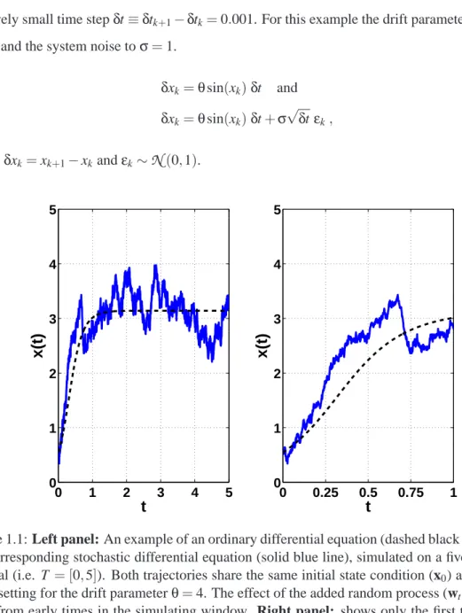
To give an example of the above discussion a simple univariate system is considered, with dynam-ics described by the following ODE (Eq. 1.8). This system is driven by a force f(xt) =θsin(xt),

and an example simulation (trajectory), on a five time unit interval, T= [0,5], is shown in Figure 1.1 (left panel, dashed black line). The corresponding SDE is given by Equation (1.9), and a real-isation with an additive noise process (i.e.σis independent of the state xt), is illustrated in Figure

1.1 (left panel, solid blue line).

dxt dt =θsin(xt) and (1.8) dxt dt =θsin(xt) +σ dwt dt (1.9)

In practice, however, the continuous time equations are transformed to their discrete time coun-terparts, as shown in Equations (1.10) and (1.11) respectively. Here a simple Euler scheme was chosen for the discretisation of both ODE and SDE (Kloeden and Platen, 1999), which imposed a relatively small time stepδt_≡δtk+1−δtk=0.001. For this example the drift parameter was set to

θ=4 and the system noise toσ=1.

δxk=θsin(xk)δt and (1.10) δxk=θsin(xk)δt+σ √ δtεk, (1.11) whereδxk=xk+1−xkandεk∼

N

t

x(t)

t

x(t)

Figure 1.1: Left panel: An example of an ordinary differential equation (dashed black line) versus the corresponding stochastic differential equation (solid blue line), simulated on a five time units interval (i.e. T = [0,5]). Both trajectories share the same initial state condition (x0) and have the same setting for the drift parameterθ=4. The effect of the added random process (wt) is obvious

even from early times in the simulating window. Right panel: shows only the first time unit of the simulation, to emphasise how fast the SDE deviates from the ODE even though they start from the exact same point.

Figure 1.1 shows that the solution for the ODE (dashed black line), is smooth and given a fixed initial condition x0, is unique. On the contrary, the solution for the SDE (solid blue line) is very rough and even though both solutions start with the same initial conditions, it deviates from the deterministic evolution in a random way. Moreover, every time that the SDE is solved the trajectory is different, as a result of the influence of the random noise process wt.

1.3

Bayesian inference

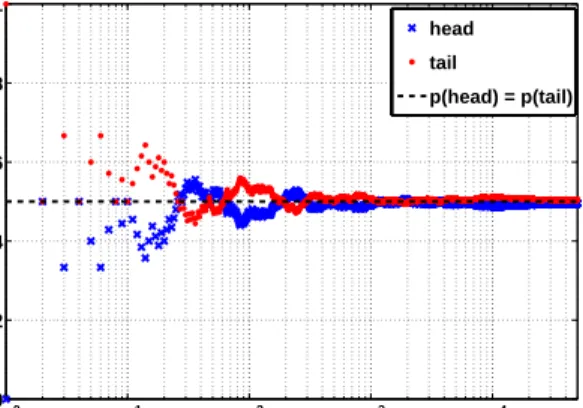
As implied earlier in Section 1.1, phenomena that appear to evolve in a random manner can be described in a probabilistic way. Shafer (1992), argues that probability can mean many things. The two most prevalent approaches, of probability theory, are the frequentist and the Bayesian interpretations. Roughly speaking, the frequentist approach interprets Kolmogorov’s Axioms for probability, as frequencies. That means the probability of an event is the long-run frequency with which the event occurs with a specific experimental setup. Figure 1.2, shows an example of the probability of appearing “Heads” (blue ’x’ symbol) or “Tails” (red circles), when tossing a fair coin. When the number of experimental trials (coin tosses) increases the probabilities of both events tend to 1/2 (horizontal dashed line), as expected for a “fair” coin.

However, the frequentist approach to probabilities requests not only for an event to have hap-pened, but also to repeat many times (infinite in theory), in order to apply a probability on that event. On the contrary, the Bayesian approach interprets the axioms as degrees of belief (i.e. probabilities can be assigned to quantify beliefs on events that have not yet happened). It is not the intention here to get involved into philosophical discussions on which probabilistic interpre-tation is correct. Within this thesis the Bayesian approach is adopted and the methods described later are developed in a Bayesian inference framework. The main reason is because within the Bayesian paradigm uncertainty, in making inference, is quantified directly by probabilities based on statistical data analysis, therefore it provides a more principled framework for its treatment.

100 101 102 103 104 0 0.2 0.4 0.6 0.8 1 number of trials frequencies head tail p(head) = p(tail)

Figure 1.2: Frequency of a “fair” coin, after 50,000 tosses. As the number of trials increases the frequency that the heads (blue ’x’ marks) and tails (red circles) appear tends to the true probability of 1/2 (horizontal dashed line).

In a Bayesian inference framework (Gelman et al., 1995), everything is expressed with prob-ability distributions. First the problem must be formulated with a “full probprob-ability model”, which is basically the joint probability density of all the quantities of interest (observed and unobserved). Then, after the prior beliefs have been quantified, in terms of prior probability density functions

(pdfs), inference can be characterised as estimating the conditional density of the quantities of interest, given the available observations. In practice, this can be achieved using Bayes’ rule1:

p(x_∣y) = p(y∣x)p(x)

p(y) , with 0<p(y)<∞, (1.12) ∝p(y_∣x)p(x). (1.13)

In Equation (1.13), p(x)is the prior density function, which incorporates all prior beliefs about the quantity x before seeing any data, p(y_∣x)is the likelihood of the observed values y given the current estimates of x, p(y)is the marginal likelihood (or evidence) which must be bounded and

p(x_∣y) is the posterior density of the quantities of primary interest conditional on the available observations.

Bayesian inference is very popular in the areas of data assimilation (Wikle and Berliner, 2007) and machine learning (Tipping, 2006), mainly because it provides a natural way to update the current estimates in the light of new observations, by iterating the Bayes rule, Eq. (1.13).

1.4

Thesis outline

Chapter 1 begins with a general discussion about the source of stochasticity (or randomness) found in real world systems and provides a small discussion, including a simple example, on the difference between a deterministic system described by an ODE and a stochastic system defined by an SDE. The viewpoint on why the Bayesian paradigm is appropriate if one wants to make inference about dynamical systems is also highlighted.

Chapter 2 gives some necessary theoretical definitions of stochastic processes, including some properties, to make the rest of the thesis more self-contained. The emphasis is on the Markov

processes and some characteristic examples are illustrated. Diffusion processes follow and the

notion of discrete time observation is clarified. The problem of optimal estimation of the system state and model parameters, given a discrete set of noisy observations is defined. Although an exhaustive review of the methodologies that deal with this problem cannot be claimed an effort is made to collect and present the basic methods on this subject.

Chapter 3 summarizes and briefly reviews the dynamical models that are used in the follow-ing chapters to validate the new approximation algorithms that developed. The univariate linear Ornstein- Uhlenbeck process (OU) is introduced and the non-linear Double-Well (DW) follows.

1_{Named after the English mathematician Thomas Bayes (1702 - 1761). Bayes theorem as described in his work,}

“An Essay towards solving a Problem in the Doctrine of Chances”, was published after his death at the ‘Philosophical Transactions of the Royal Society of London (1763).

To test how the methods developed scale to multivariate systems a stochastic version of the three dimensional chaotic Lorenz ’63 system (L3D) is implemented. The last system considered is the forty dimensional stochastic Lorenz ’96 (L40D).

Chapter 4 reviews in detail the variational Gaussian process approximation (VGPA) algorithm, for partially observed diffusions that was first introduced in Archambeau et al. (2007). This is essential because the VGPA algorithm provides the backbone of both extensions that will follow in the next chapters. The state estimation (smoothing) framework is examined first, with two approaches to estimating the model (hyper) parameters following.

Chapter 5 presents an extension of the aforementioned VGPA algorithm in terms of basis func-tion expansions defined globally over the whole time domain of the inference window. Initially, the main characteristics and benefits of using RBFs are highlighted and then the general multivari-ate framework is derived. Numerical simulations test its convergence properties comparing to the original VGPA algorithm and results of estimating (hyper-) parameters are also included.

Chapter 6 provides an alternative re-parametrisation of the original VGPA framework by using polynomial approximation defined locally between each pair of observations. This approach al-though similar to the one of the basis function expansions, as presented in Chapter 5, gives a more appropriate approximation framework with beneficial characteristics.

Chapter 7 compares the previously derived extensions with a variety of well known methods of state and parameter estimation. The algorithms are briefly described and the comparison results are presented separately for state and parameter estimation. The asymptotic properties of the local polynomial approximation (as defined in Chapter 6), as the number of observations or length of time window increases, is empirically thoroughly analysed.

Chapter 8 summarizes the work and provides possible future research directions.

1.5

Disclaimer

This thesis is submitted for the degree of Doctor of Philosophy (Ph.D). The work presented here is original and has not been submitted previously for a degree, diploma or qualification at another university. However, parts of the work have been published and presented in the following papers, conferences and seminars (in chronological order):

∙ Appendix A, which contains the full derivations of the original VGPA framework, has been submitted as a Non-linearity and Complexity Research Group (NCRG) technical report in Vrettas et al. (2008).

∙ Early theoretical work on both extensions, as described in Chapters 5 and 6, has been ac-cepted and presented at the Bayesian Inference for Stochastic Processes (BISP) workshop, June, 2009.

∙ The complete theoretical framework (for the univariate case) of the basis function expan-sion (Chapter 5), along with some preliminary results on the univariate DW system have been presented at the European Symposium on Artificial Neural Networks (ESANN) and published in the conference proceedings (Vrettas et al., 2009). In addition, an extended version of the paper containing the full multivariate RBF framework and results on higher-dimensional systems has been published in Neurocomputing (Vrettas et al., 2010b).

∙ Comparison results, mainly on state estimation, of the VGPA algorithm with methods im-plemented in Chapter 7, have been presented at the European Geosciences Union (EGU) conference, April 2010.

∙ The local polynomial extension along with many results included in Chapters 6 and 7, have been submitted as a journal paper to Physica D (Vrettas et al., 2010a).

∙ Finally, many views and approaches presented here have been discussed in the Non-linearity and Complexity Research Group (NCRG, Aston University) seminars, on several occasions.

2

existing methodologies

2.3 Partially observed diffusions . . . . 26 2.4 Problem definition . . . . 27 2.5 Existing methodologies . . . . 28 2.5.1 Sequential approaches . . . 28 2.5.2 MCMC approaches . . . 29 2.5.3 Variational approaches . . . 30 2.5.4 Non-Bayesian approaches . . . 31 2.6 Discussion . . . . 33

“Probable is what usually happens.” — Aristotle, Greek philosopher.

2.1

Foreword

Chapter 2 introduces the reader to the problem this thesis addresses, as well as the main categories of methodologies that have been developed to solve it. In order to do that it is necessary to first give a review of the main mathematical elements that are used later to built the machinery of the approximation methods that developed. A basic level of probability theory is assumed (e.g. events, sample spaces, probabilities, etc.). Instead of rigorous definitions, intuitive ways of presenting the essential building blocks are preferred. A more detailed presentation on the subject of probability theory and stochastic processes is given by Papoulis (1984).

2.1.1 Chapter outline

The chapter is organised as follows. Initially a definition of a stochastic process is given, includ-ing some useful properties. Emphasis is on so-called Markov processes and some characteristic examples such as the Gaussian and the Wiener processes are illustrated. The important class of diffusion processes follows and the notion of discrete time observation is clarified. After the basic elements are introduced, the inference problem (from a Bayesian perspective) that provides the focus of this work is properly defined. A review of the methods that address inference in partially observed diffusion processes is given. The chapter concludes with a discussion.

2.2

Stochastic processes

Stochastic processes (also known as random processes) arise naturally in range of different con-texts from financial modelling (e.g. the stock market, exchange rate fluctuations), biological mod-elling (e.g. a patient’s EEG) to environmental modmod-elling (e.g. the temperature at a point). It can be seen intuitively as a physical phenomenon which evolves in time in a random or, in a loose sense, probabilistic way. In this section a definition of a stochastic process will be given, highlighting some important properties as well as providing an intuitive view, based on some characteristic examples. It is not the intention to reproduce all the theory around stochastic processes (which would require proper It¯o calculus). Instead it only provides the basic definitions and properties that are necessary for the rest of the thesis. An informal and short introduction to stochastic processes can be found in Miller (2007). For a more complete and detailed study of the subject there are excellent textbooks such as Honerkamp (1993); Gardiner (2003), and Kloeden and Platen (1999), where all the concepts are provided in a formal mathematical manner.

Definition 2.2.1 A stochastic process is a collection of random variables,(xt), indexed by a set,

which here is interpreted as time. Hence if T_⊂ℜ, is the time set under consideration and(Ω,A,P)

a common probability space, then_{xt}t_∈T is a stochastic process.

Thus, it can be seen as a function of two variables T_×Ω_→ℜsuch that:

∙ x(t,_⋅):Ω_→ℜis a random variable_∀t_∈T .

∙ x(_⋅,ω): T _→ℜis a realization_∀ω_∈Ω.

If T is a countable set (discrete case) the stochastic process is called discrete in time, otherwise if

T is an interval (continuous case) the stochastic process is known as continuous in time.

Some important properties, that can characterise whole classes of stochastic processes are:

Property 2.2.1 Given a partition of time, T =_{t1<t2<⋅⋅⋅<tn}and a positive quantity d>0,

a stochastic process is strictly stationary if, _∀t_∈T the joint distributions(xt1,xt2, . . . ,xtn)and

(xt1+d,xt2+d, . . . ,xtn+d)are identically distributed. That is, time displacements leave the joint

dis-tributions unchanged.

Property 2.2.2 Given a partition of time, T =_{t1<t2<⋅⋅⋅<tn}, a stochastic process is said to

have independent increments if,_∀t_∈T the random variables (xtj+1−xtj), with j=1,2, . . . ,n−1

are independent for any finite combination of time instants.

Property 2.2.3 If, for any t >s and d>0, the distribution of (xt+d−xs+d) is the same as the

distribution of (xt−xs), then the process is said to have stationary independent increments. Property 2.2.4 A stochastic process in which if one wants to make a prediction about the state of

the system, at a future time ‘tn+1’, the only information necessary is the state of the system at the

present time ‘tn’, is called a Markov process.

Any knowledge about the past (of a Markov process) is redundant. More accurately this is called a “first order” Markov process. This can be generalised to “m’th order” by allowing the process to “remember” the m₋1 past states. However for the rest of this thesis emphasis is only on “first order” Markov processes unless stated otherwise.

2.2.1 Examples Gaussian Processes

One of the most well known classes of stochastic processes is the Gaussian process. Here the index set is (often) not considered as the time. A thorough treatment of Gaussian processes can be

found in Rasmussen and Williams (2006). Here the formal definition as given in Rasmussen and Williams (2006, Ch.2) is adopted.

Definition 2.2.2 “A Gaussian process is a collection of random variables, any finite number of

which have a joint Gaussian distribution.”

The Gaussian process can be fully characterised by its first two moments. For a multivariate process that is:

∙ means : 𝝁t=⟨xt⟩,∀t∈T . ∙ variances :𝝈2 t = 〈 (xt−𝝁t)(xt−𝝁t)⊤ 〉 ,_∀t_∈T .

∙ (two-point) covariances : cov(s,t) =〈(xs−𝝁s)(xt−𝝁t)⊤

〉

,_∀t,s_∈T with t_∕=s.

Wiener Process

A well studied Gaussian process is the Wiener process1. It is a continuous-time stochastic process which was proposed to describe the arbitrary movement of a particle pollen on the surface of water, due to the continuous collisions with many water molecules, and is also known as Brownian motion or a continuous random walk.

Definition 2.2.3 A Wiener process is a continuous-time Gaussian process that satisfies the Markov

property, with independent increments for which:

∙ w0 = 0 , with probability 1 ∙ ⟨wt⟩ = 0 ∙ wt−ws∼

N

Figure 2.1(a) shows four sample paths, or trajectories, from the standard univariate Wiener process. Notice that although a Wiener sample path is a continuous function of time almost surely, it is not differentiable with probability one; this is called a rough process.

0 1 2 3 4 5 6 7 8 9 10 −4 −2 0 2 4 6 8 t w(t)

(a) 1D Wiener process

−3 −2 −1 0 1 2 −4 −3 −2 −1 0 1 w x(t) w y (t) (b) 2D Wiener process

Figure 2.1: (a) Four different standard Wiener paths are simulated, each one presented with dif-ferent colour. (b) An illustration of a two dimensional Wiener process. Note that all sample paths start at w0=0.

2.3

Partially observed diffusions

Diffusion processes are a special class of continuous time Markov processes with continuous sam-ple paths, (Kloeden and Platen, 1999). The time evolution of a general, D dimensional, diffusion process_{xt}t∈Tcan be described by a stochastic differential equation (here to be interpreted in the

It¯o sense):

dxt=f(t,xt;𝜽)dt+Σ(t,xt;𝜽)1/2dwt, dwt ∼

N

where xt∈ℜDis the D dimensional latent state vector, f(t,xt;𝜽)∈ℜDis the (typically) non-linear

drift function, that models the deterministic part of the system,Σ_{(t,xt;𝜽)∈}ℜD×D_{is the diffusion} or system noise covariance matrix and dwt is the differential of a D dimensional Wiener process, {wt}t_∈T, which often models the effect of faster dynamical modes not explicitly represented in the

drift function but present in the real system. T = [t0,tf]is a fixed time window of inference, with

t0and tf denoting the initial and final times respectively. The vector𝜽∈ℜmis a set of parameters

within the drift and diffusion functions.

Necessary conditions

To be a diffusion process the following limits must exist for all 0_≤s<t, withδ>0 (Kloeden and Platen, 1999): lim t→s [ (t₋s)−1 ∫ ∣z−x∣>δp(s,x;t,z)dz ] =0 (2.2) lim t_→s [ (t₋s)−1 ∫ ∣z−x∣≤δ(z−x)p(s,x;t,z)dz ] = f(s,x) (2.3) lim t→s [ (t₋s)−1 ∫ ∣z−x∣≤δ(z−x)(z−x) ⊤_p(s,x;t,z)dz ] =Σ_{(s,x) (2.4)} where x, z _∈ℜD, p(s,x;t,z) is the transition pdf and the dependence of the drift and diffusion functions on the parameters𝜽 has been omitted for notational brevity. The first limit Eq. (2.2)

prevents the process from having large displacements over a small time interval. Conditions (2.3) and (2.4) are the instantaneous rate of change in the mean (drift function) and covariance (diffusion coefficient), given that the process was at state x at time s (i.e. x(s)_≡xs=x).

Discrete observations

Often the latent process is only partially observed, at a small number of ordered discrete times

{tk}Kk=1, which satisfy : t0<t1<t2<⋅⋅⋅<tK <tf. In addition the observations are subject to

error. Hence

yk=h(xtk) +𝝐k, 𝝐k∼

N

where yk∈ℜd denotes the k’th observation taken at time tk, h(⋅):ℜD→ℜd is the general

obser-vation operator and the obserobser-vation noise𝝐k∈ℜd, is assumed (for simplicity) to be independent

and identically distributed (i.i.d.) Gaussian white, with covariance matrix R_∈ℜd×d. Note that if the nature of the observations varies at different times then hk(⋅)is used instead.

2.4

Problem definition

This thesis addresses the problem of inferring the states of a system (xt), together with the

(pos-sibly) unknown model parameters (𝜽), from systems that are modelled by diffusion processes and observed at a finite set of discrete time points.

This is an interesting and challenging task because diffusion models have been used exten-sively in the last few decades to model phenomena that exhibit randomness and evolve continu-ously in time. Meanwhile, observations from most physical systems arrive at discrete times (e.g. hourly, daily, monthly, etc.).

More precisely, one is dealing with a continuous time system, which is observed at discrete times; and that is what makes the problem difficult. In all but a few examples1, estimation of dif-fusion models is not straightforward because the SDE that describes the temporal evolution of the system cannot be solved analytically. Moreover, most real world processes are complex, which implies a non-linear drift f(xt) and diffusion function is necessary, if good agreement with the

measurable values is to be achieved. This complicates the statistical analysis even more because the (discrete-time) transition densities Eq. (2.2) are no longer tractable, which means that estima-tion of the model parameters within a tradiestima-tional Maximum-Likelihood (ML) framework is not possible. Therefore, approximate techniques are sought.

1_{(a) Geometric Brownian motion, (b) Ornstein-Uhlenbeck process and (c) Cox-Ingressol-Ross process, have}

In a Bayesian framework, the goal is: given a system whose evolution is described by a dif-fusion (such as Equation 2.1) and a set of discrete time observations (Equation 2.5) to estimate the (smoothing) posterior distribution, ps(xt∣y1:K), conditioned on the available observations. The system states might be summarised as the mean mt=⟨xt⟩ps, together with a measure of its

uncer-tainty St =

〈

(xt−mt)(xt−mt)⊤

〉

ps. In addition, when the model parameters𝜽are unknown, an

estimate of their value is also desirable.

2.5

Existing methodologies

After describing the main inference problem addressed in this thesis, the current section reviews and discusses the main methodologies that have been employed to solve it. Inference for non-linear stochastic dynamical systems, which are observed at a finite set of discrete time instants, is a challenging task because the missing paths between observed values must also be estimated, together with any unknown parameters.

A variety of different approaches has been developed to undertake inference in SDEs. This thesis focuses largely on Bayesian approaches which from a methodological point of view can be grouped into the following three main categories: (a) sequential, (b) Markov chain Monte Carlo (MCMC) and (c) variational approaches. Note that this classification is not unique and others are possible.

2.5.1 Sequential approaches

The first category attempts to solve the Kushner-Stratonovich-Pardoux (KSP) equations (Kushner, 1967a). The KSP method (described briefly in Eyink et al. (2004)), can be applied to give the optimal (in terms of variance minimising estimator) Bayesian posterior solution to the inference problem, providing the exact conditional statistics (often expressed in terms of the mean and co-variance) given a set of observations and serves as a benchmark for other approximation methods. Initially, the optimal filtering problem was solved by Kushner and Stratonovich (Stratonovich, 1960; Kushner, 1962, 1967a) and later the optimal smoothing setting was given by an adjoint (backward) algorithm due to Pardoux (1982). Unfortunately, the KSP method is computationally intractable when applied to high dimensional non-linear systems (Kushner, 1967b; Miller et al., 1994), hence a number of approximations have been developed to deal with this issue.

For instance, when the problem is linear the filtering part of the KSP equations (i.e. the forward Kolmogorov equations) boil down to the Kalman and Bucy (1961) filter, which is the continuous time version of the well known Kalman filter (Kalman, 1960). When dealing with systems that exhibit non-linear behaviour a variety of approximations, based on the original Kalman filter (KF),

have been proposed to overcome these difficulties. The first approach is to linearise the model (usually up to first order) around the current state estimate, which through a Taylor expansion, requires the derivation of the Jacobian of the model evolution equations. However, this Jacobian might not always be easy to compute. Moreover the model should be smooth enough in the time-scales of interest, otherwise linearisation errors will grow causing the filter estimates to diverge. This method is known as the extended Kalman filter (EKF) (Maybeck, 1979) and was succeeded by a family of methods based on statistical linearisation exploiting the observation that it is easier to approximate a probability distribution than a non-linear operator.

A widely used method that has produced a large body of literature is the ensemble Kalman fil-ter (EnKF) (Evensen, 2003), or when dealing with the smoothing problem the ensemble Kalman smoother (EnKS) (Evensen and van Leeuwen, 1999). Recently another strategy has proposed that rather than sampling this ensemble of particles randomly from the initial distribution it is prefer-able to select a design (i.e. deterministically chose them), so as to capture specific information (usually the first two moments), about the distribution of interest. This method is often called the

unscented transform and the filtering method is thus referred to as the unscented Kalman filter

(UnKF), first introduced by Julier et al. (2000). Another popular, approach is the particle filter by Kitagawa (1987), in which the solution of the posterior density (or KSP equations) is approxi-mated by a discrete set of particles with random support (Kivman, 2003; Fearnhead et al., 2008). This method can be seen as a generalisation of the ensemble Kalman filter, because it does not make the Gaussian assumption when the ensemble is updated in the light of the observations. In other words, if the dynamics of the system are linear then both filters should give the same answer, given a sufficiently large number of particles (ensemble) members.

2.5.2 MCMC approaches

The second category applies Monte Carlo methods to sample from the posterior process, focusing on areas (in the state space) of high probability, based on Markov chains (Neal, 1993). When the dynamics of the system is deterministic, then the sampling problem is on the space of initial conditions. In contrast, when the dynamics is stochastic the sampling problem is on the space of (infinite dimensional) sample paths. Therefore MCMC methods for diffusions are also known as “path-sampling” techniques. Although early sampling techniques such as the Geman and Geman (1984) Gibbs sampler can be applied to systems, convergence is often too slow. In order to achieve better mixing of the chain and faster convergence other more complex and sophisticated techniques were developed. Stuart et al. (2004), introduced the Langevin MCMC method, which essentially generalises the Langevin equation to sampling in infinite dimensions. A similar approach is the

sampling problems by Alexander et al. (2005). Both algorithms (Langevin MCMC and HMC) need information on the gradient of the target log-posterior distribution and update the entire trajectory (sample path) at each iteration. They combine ideas of molecular dynamics, employing the Hamiltonian of the system (including a kinetic energy term), to produce new configurations which are then accepted or rejected in a probabilistic way using the Metropolis criterion.

Following the work of Pedersen (1995), on simulated maximum likelihood estimation (SMLE), Durham and Gallant (2002) examine a variety of numerical techniques to refine the performance of this method by introducing the notion of the Brownian bridge, between two consecutive obser-vations, instead of the Euler discretisation scheme that was used in Pedersen (1995). This lead to various “blocking strategies”, for sampling the sub-paths, such as the one proposed by Golightly and Wilkinson (2006), as an extension to the previous “modified bridge” (Durham and Gallant, 2002). The work of Elerian et al. (2001); Eraker (2001) and Roberts and Stramer (2001) is based on a similar direction, that is augmenting the state with additional data between the measured values, in order to form a complete data likelihood and then use a Gibbs sampler or other sam-pling techniques (e.g. MCMC). A rather different samsam-pling approach is presented by Beskos et al. (2006b), where an “exact sampling” algorithm (in the sense that there are no discretisation errors), is developed that does not depend on data imputation between the observable values, but rather on a technique called retrospective sampling (see Papaspiliopoulos and Roberts (2008) for further details). Although this method is very appealing and computationally efficient compared to other sampling methods that depend on fine temporal discretisation to achieve sufficient accuracy, the applicability of the method depends heavily on the exact algorithm, as introduced by Beskos et al. (2006a).

2.5.3 Variational approaches

The final category (from a Bayesian point of view) of methodologies approximates the posterior process using variational techniques (Jaakkola, 2001). A popular methodology, which is opera-tional at the European Centre for Medium-Range Weather Forecasts (ECMWF), is the four di-mensional variational data assimilation method, also known as “4D-Var” (Dimet and Talagrand, 1986). This method seeks the most probable trajectory (or the mode), of the approximate poste-rior smoothing distribution, within a predefined time window. This is found by minimising a cost function which depends on the measured values and the model dynamics. However, this method does not provide uncertainty estimates around the most probable solution. The “4D-Var” method, as adopted by the ECMWF and others, makes the strong assumption that the model is either per-fectly known, or that any uncertainties are negligible and hence can be ignored. A generalisation of this strong perfect model assumption, is to accept that the model is not perfect and should be

treated as an approximate solution to the real equations governing the system. This leads to a

weak formulation of 4D-Var as described in Derber (1989); Zupanski (1996). The theory behind

the weak formulation was introduced in early 70’s by Sasaki (1970) - several versions are described in Tremolet (2006) and will be discussed later.

Another variational technique that seeks the conditional mean and variance of the posterior smoothing distribution is described in Eyink et al. (2004). In this work Eyink, argues that the ultimate goal of a data assimilation method is to recover not a specific history that generated the observations, but rather the correct posterior distribution, conditioned upon the observations. To achieve that a mean field approximation is applied to the KSP equations, which as discussed earlier provides the optimal filtering and smoothing solution to the inference problem, from a Bayesian perspective. More recently the work of Archambeau et al. (2007), suggested a rather different approach, where the true posterior process is approximated by a time-varying linear dynamical system (such as a non-stationary Gaussian process), rather than assuming a fully factorising form to the joint posterior. This linear approximation assumption implies a fine time discretisation, if good accuracy is to be achieved, and tries to optimise globally the approximate posterior process in terms of minimising the Kullback-Leibler divergence (Kullback and Leibler, 1951), between the two probability measures. This method is further reviewed in Chapter 4.

2.5.4 Non-Bayesian approaches

Although, this thesis addresses the inference problem from a Bayesian perspective, to provide a more complete overview of the proposed methodologies, this section reviews briefly the main non-Bayesian estimation techniques (for reviews see Nielsen et al. (2000) and Sorensen (2004)), that have been developed for inference in partially observed diffusion processes. In general, the methods cited here focus largely in estimating the model parameters (i.e. unknown parameters in the drift and diffusion functions) and can be grouped into: (i) analytical and numerical approx-imations of the true likelihood, (ii) estimating functions and (iii) indirect inference and efficient method of moments (EMM).

The most appealing methods are those that approximate the true likelihood. This approxima-tion can, theoretically, be made arbitrarily accurate. There are three main types: The first one provides numerical solutions to the Fokker-Planck equation (which is a partial differential equa-tion)1and was initially recognised by Lo (1988). Later, various implementations were introduced by Hurn and Lindsay (1997) using spectral approximations and Jensen and Poulsen (2002) us-ing the method of finite differences. The second method obtains estimates of the true likelihood via simulations (Pedersen, 1995; Brandt and Santa-Clara, 2002; Hurn et al., 2003). A common

characteristic of these approaches is the use of a numerical scheme (such as the Euler) to move from one state of the system xk, at time tk, to the next state xk+1, at time tk+1, in n time steps. Even with efficient modern computers both numerical approaches are quite computationally de-manding. The third approach provides analytical, yet very accurate, discrete approximations to the likelihood function (Florens-Zmirou, 1989; Shoji and Ozaki, 1997; Ait-Sahalia, 1999, 2002). The core idea behind these methods is to replace the true transition density with another that has closed-form solutions and includes the (hyper-) parameters 𝜽 of the SDE (Equation 2.1). The simplest case is to use as a proxy for the true transition pdf the Gaussian distribution such as

N

compli-cated even for low order approximations. Moreover, the bias that is introduced due to the discrete time approximation makes the estimates of the parameters inconsistent for any fixed sampling interval.

Estimation via estimating functions is generally faster (Jacobsen, 2001). Roughly speaking, an estimation function is defined as F(y,𝜽):ℜp_→ℜ, where its arguments are the observations y and the model parameters𝜽. The property of this function is that it goes to zero as the parameters 𝜽 tend to their optimal values (i.e. F_→0 as𝜽_→𝜽opt). An example is the score function

yield-ing the maximum likelihood estimator. However, for the SDEs the score function is not available therefore alternative solutions are sought. The so called simple estimating functions are available in explicit form but provide only estimators for parameters from the marginal distribution (Kessler and Sorensen, 1999; Sorensen, 2000). Still, they may be useful for preliminary analysis, for ex-ample in combination with martingale estimating functions. The latter are analytically available for a few models but in general they must be simulated (Bibby and Sorensen, 1995). This basi-cally amounts to simulating conditional expectations, which is faster than calculating conditional densities as required by the numerical likelihood approximations mentioned above.

Indirect inference (Gourieroux et al., 1993) and EMM (Gallant and Tauchen, 1996), which is closely related to the General Methods of Moments (Hansen, 1982; Hansen and Scheinkman, 1995; Duffie and Singleton, 1993), introduce discrete time auxiliary (usually wrong) models to ap-proximate the true models. Then, the model parameters of the auxiliary model (e.g.𝝃) are linked to the true parameters𝜽with the so-called binding function (i.e.𝝃=ν(𝜽)). Subsequently, maximum likelihood estimates are obtained for the auxiliary (proxy) model ξML and the estimates for the

true parameters are obtained using the inverse of the binding function (i.e. ˆ𝜽=ν−1₍ξ

ML)).

Never-theless, the quality of the estimators depends heavily on the auxiliary model which, in essence, is chosen arbitrarily.

Most of the aforementioned methods are, in principle, applicable to multivariate diffusions as well. With a few exceptions this has yet to be demonstrated in practice. Moreover, the

compu-tational cost will be even more substantial than for univariate processes. A more comprehensive review for these methods can be found in Jeisman (2005).

2.6

Discussion

This chapter initially introduced the main building blocks that are used extensively later in the thesis. An informal definition of stochastic processes, along with some useful properties and some simple characteristic examples (i.e. the Gaussian and Wiener process), are also provided. A thorough mathematical description of stochastic processes that would require proper stochastic calculus is avoided. Instead a more practical approach is followed and relevant references are cited.

The importance of partially observed diffusions was highlighted. The necessary limit con-ditions that distinguish them from the other families of the stochastic processes were given and assumed to be satisfied for all the examples in the thesis. Furthermore, the notion of discrete observations was further clarified.

Defining the problem addressed in the thesis is of great importance. The difficulty of obtaining estimates of the system’s states together with unknown model parameters was stressed and the major methodologies to tackle this problem were reviewed. Although a complete list of references is not claimed the effort was to gather the most well known and widely accepted methods. In spite of the fact that the inference problem here is placed within a Bayesian framework, alternative (non-Bayesian) approaches that deal with the estimation of parameters in SDEs were also reviewed.

3

Systems studied

CONTENTS

3.1 Foreword . . . . 35

3.1.1 Chapter outline . . . 35

3.2 The Ornstein-Uhlenbeck process . . . . 35 3.3 The double well system . . . . 38 3.4 The Lorenz ’63 (3D model) . . . . 39 3.5 The Lorenz ’96 (40D model) . . . . 40 3.6 Discussion . . . . 42

“Essentially, all models are wrong, but some are useful.” — George E. P. Box, English statistician.

3.1

Foreword

When developing new methodologies to solve the inference problem, as described in Chapter 2, it is important to validate them on dynamical systems (or models) with known properties and broad acceptance from the scientific community as benchmark models, before applying them to real world problems. However, to