Fragmented protein sequence alignment using
two-layer particle swarm optimization (FTLPSO)
Nourelhuda Moustafa
a,*, Moustafa Elhosseini
a, Tarek Hosny Taha
b,
Mofreh Salem
aa
Computers Engineering & Control Systems Dept., Mansoura University, P.O. box: 35516, Egypt b
City for Scientific Research and Technology Applications, Environmental Biotechnology, P.O. box: 21934, New Borg El-Arab, Egypt
Received 25 November 2015; accepted 23 April 2016
KEYWORDS
Multiple sequence alignment; Particle swarm optimization; Fragmentation;
Two-layer PSO
Abstract This paper presents a Fragmented protein sequence alignment using two-layer PSO (FTLPSO) method to overcome the drawbacks of particle swarm optimization (PSO) and improve its performance in solving multiple sequence alignment (MSA) problem. The standard PSO suffers from the trapping in local optima, and its disability to do better alignment for longer sequences. To overcome these problems, a fragmentation technique is first introduced to divide the longer datasets to a number of fragments. Then a two-layer PSO algorithm is applied to align each fragment, which has ability to deal with unconstrained optimization problems and increase diversity of particles. The proposed method is tested on some Balibase benchmarks of different lengths. The numerical results are compared with CLUSTAL Omega, CLUSTAL W2, TCOFFEE, KALIGN, and DIALIGN-PFAM. It has been shown that better alignment scores have been achieved using the proposed tech-nique FTLPSO. Further, studies on PSO update equation’s parameters and the parameters of the used scoring functions are presented and discussed.
Ó2016 Production and Hosting by Elsevier B.V. on behalf of King Saud University. This is an open access article under the CC BY-NC-ND license (http://creativecommons.org/licenses/by-nc-nd/4.0/).
1. Introduction
Bioinformatics is an interdisciplinary field which studies com-bining aspects of biology, mathematics, and computer science. The bioinformatics can develop and improve methods for stor-ing, retrievstor-ing, organizing and analyzing biological data (Cohen, 2004). A major activity in bioinformatics is to develop software tools to generate useful biological knowledge. One of the very important areas in bioinformatics is sequence align-ment. The first step of creating phylogenetic trees is comparing sequences, grouping them according to their degree of similar-ity using alignment. Determination of the consensus sequence * Corresponding author. Tel.: +20 1116688052.
E-mail addresses:[email protected],nour.alhuda762@gmail. com(N. Moustafa),[email protected](M. Elhosseini), t.h.taha @gmail.com(T.H. Taha),[email protected](M. Salem). Peer review under responsibility of King Saud University.
Production and hosting by Elsevier
King Saud University
Journal of King Saud University –
Science
www.ksu.edu.sa
of several aligned sequences can help develop a finger print sequence which allows the identification of members of dis-tantly related protein family. Most recent protein secondary structure prediction and analysis methods also use sequence alignments to improve the prediction quality (Di Francesco et al., 1996; Jagadamba et al., 2011).
Sequence alignment is used to arrange the sequences of DNA, RNA, or protein to identify regions of similarity. When regions of similarities between aligned sequences increase, it gives information that there is a similarity between these sequences in their function, their secondary and tertiary struc-ture (Cohen, 2004). Solving the sequence alignment problem depends on gap insertion (Katoh and Standley, 2016). The gap should be inserted in correct places such that the align-ment can achieve high residue matching and high scores Align-ment problem may be applied on only two sequences, called pairwise alignment, PWA (Agrawal and Huang, 2009; Sierk et al., 2010), or on more than two sequences, called multiple sequence alignment, MSA (Sievers et al., 2011; Subramanian et al., 2008).
The optimization problem of the MSA is used to be solved using dynamic programming (Needleman and Wunsch, 1970; Smith and Waterman, 1981), and progressive methods (Al Ait et al., 2013; Lalwani et al., 2015). However, problems of high processing and high memory usage may be faced with no guarantee that the system will reach the optimal solution. The new trend is using iterative approach techniques due to their simplicity, and ability to solve multidimensional opti-mization problems in many fields (Das et al., 2008; Kiranyaz et al., 2009). Particle swarm optimization (PSO) is a swarm intelligent technique which proves its ability in solving MSA problem. However, the PSO suffers from the trapping of par-ticles in local optima. Moreover, the PSO algorithm can han-dle short sequences in an efficient way, but increasing sequence lengths lead to decreasing solution accuracy. The main targets of this paper are to:
– Pave the way for PSO to deal with different sequence lengths.
– Give PSO the ability to solve MSA problems and achieve high scores.
– Make PSO safe from falling in a local optimal point as possible.
To achieve these goals, fragmentation is proposed to shorten the long sequences, and to let the swarm focus on find-ing the optimal solution of the small fragment within a small search space, which has a less number of local optimal solu-tions. Then, a PSO variant is selected to align each fragment alone. This variant is two-layer PSO (TLPSO). It is selected due to its ability to solve unconstrained problems such as MSA. These two layers contain many swarms: R swarms in the first layer, and one swarm in the second layer. Particles in every swarm are dealing with each other using Local-PSO variant as a way to give the particles more ability to reach the optimal solution without trapping in a local optima. Finally, mutation is used to give more help to the swarm if it has been trapped.
The rest of paper is organized as follows: the history of alignment problem is mentioned in Section 2, followed by the alignment scoring functions in Section 3. A description of particle swarm optimization technique is illustrated in
Section4. The proposed algorithm is introduced in Section5. Finally, the computed results with discussion, followed by some parametric studies are presented in Section6.
2. Related work
Many methods are presented to solve alignment method such as dynamic programming, progressive, consistency-based, and iterative methods.
Dynamic programming technique creates a matrix of n -dimensions for nsequences. The matrix is filled with scores by some calculations, and then the optimal path can be found. The dynamic programming technique gives an optimal align-ment score, but it depends on the number of sequences n. Therefore, the computational time and memory usage will be increased by increasing thenvalue. So, dynamic programming can’t be used for more than two sequences practically although it can align multiple sequences theoretically (Suresh and Vijayalakshmi, 2013).
Progressive alignment is used to align multiple sequences, by aligning each two sequences together, creating a guide tree based on the similarity score of each two pairs, and aligning all sequences one by one. One of the first and most famous
pro-gressive alignment methods is CLUSTAL W (Thompson
et al., 1994). One disadvantage of a progressive alignment is that the algorithm is greedy. This means that the alignment depends on the early aligned pair of sequences. Therefore, any early happened mistake will affect the rest of the progres-sive alignments. Also the time to perform such progresprogres-sive alignments is proportional to the number of sequences (Lalwani et al., 2013b). To overcome the greedy problem, CLUSTAL W2 (Larkin et al., 2007) does a progressive align-ment many times using different gap penalty scores, and
accepts the best score. KALIGN (Lassmann and
Sonnhammer, 2005) also follows the standard progressive
alignment except it depends on Wu–Manber (Wu and
Manber, 1992) as a pairwise distance estimator instead ofk -tuple used by CLUSTAL.
Another approach is a consistency based approach, which depends on the principle of maximizing the agreement of pair-wise alignment. It looks for an agreement in which the created tree gives high accuracy when used for further progressive alignment. DIALIGN (Morgenstern et al., 1996), and TCOF-FEE (Notredame et al., 2000) are two examples of consistency based algorithm. DIALIGN combines local and global align-ment features. It depends on discovering local homologies among sequences, as discovering conserved (functional) regions. Many variants of DIALIGN are presented including
Anchored DIALIGN (Morgenstern et al., 2006) and
DIALIGN-TX (Subramanian et al., 2008). The newest variant depends on PFAM database (Finn et al., 2008) which collects protein families, in which these families are represented by
multiple sequence alignment. This variant is called
DIALIGN-PFAM (Al Ait et al., 2013). TCOFFEE depends on creating libraries of both global and local pairwise align-ment as a step to do multiple sequence alignalign-ment.
Because dependency on consistency based approach alone does not guarantee the accuracy of the alignment, post processing using iterative refinement is used to improve the
performance of progressive alignment. MAFFT (Katoh
of progressive-iterative approach. Every iteration they update the tree and re-do MSA until there is no improve-ment in the score. Computational intelligence techniques also used to enhance the alignment results given by progres-sive alignment techniques (Pankaj and Pankaj, 2013; Suresh and Vijayalakshmi, 2013). Other approach is probabilistic consistency transformation based strategy (using HMM),
which is used from many tools such as probcon (Do
et al., 2005), probalign (Roshan and Livesay, 2006), and CLUSTAL Omega (Sievers et al., 2011). This approach is used to decide the probability of distribution for every pair-wise alignment done on the whole sequences of the database before the creation of the tree.
While probabilistic consistency, and progressive-iterative refinement approaches give accurate results, their computa-tions are complex (Mount, 2004), and their memory usage is high (Pais et al., 2014). On the other hand, iterative approach based computational intelligence techniques overcome pro-gressive approach, which gives equality in priority to all sequences. Therefore, accurate alignment results can be achieved using simple computations (Arulmani et al., 2012; Lalwani et al., 2013b). Many papers tried to solve the problem using iterative approach only, like simulated annealing (Kim et al., 1994), Genetic algorithm (Botta and Negro, 2010; Notredame and Higgins, 1996), and particle swarm optimiza-tion (Xu and Chen, 2009; Long et al., 2009a, 2009b; Lalwani et al., 2013b; Lalwani et al., 2015).
Simulated annealing was too slow but it works well as an alignment improver. For small numbers of sequences, genetic algorithm (GA) is a better alternative for finding the optimal solution. However, as the number of sequences increases, it can fall behind optimal solutions and exponential growth in time may be observed. PSO proves its superiority in speed con-vergence than simulated annealing, and its ability to align number of sequences larger than genetic algorithm. In addi-tion, PSO has a few numbers of parameters that need tuning and parameter setting (Lalwani et al., 2013a). Standard PSO performance in short sequences is better than long ones (Xu and Chen, 2009; Long et al., 2009a; Long et al., 2009b). Then, TLPSO with mutation is proposed for the first time byChen (2011), and tested on nine optimization problems, and proves its ability to get the optimum solution. For MSA, TLPSO (Lalwani et al., 2015) is tested with creation of new swarm every iteration, as a way for mutation, and proves its superior-ity than standard PSO. However, more enhancements on PSO are still needed to reach the optimal solution especially for long sequences.
In this paper, theFTLPSO is proposed. A fragmentation technique based on k-tuple is applied to shorten the long sequences to small sub-sequences, aiming to solve the prob-lems of PSO. Then, TLPSO is applied as a suitable variant for MSA problem.
3. Scoring functions for MSA
The performance of the alignment process is measured by scor-ing functions which reflect the accuracy of the alignment. The most used two scoring functions are:
- Column Score (CS) score is used to increase the number of matched columns:
For the aligned dataset of n sequences, and alignment lengthAL, the scoring function is calculated for every column of positionxas:
CS¼X AL
x¼1
mt ð1þ ðmt=nÞÞ ð1Þ
wheremtis the number of matched residues.
– Sum of Pair (SOP) score is applied to increase the similarity match between every two sequences:
For an aligned dataset ofnsequences, the scoring function is calculated for every two sequencesSi; Sjas shown in Eq.(2):
Pairwise alignment score¼X
AL
x¼1
scoreðSiðxÞ;SjðxÞÞ ð2Þ
where: for every two characters at the same positionx, the score ofðSiðxÞ;SjðxÞÞis calculated as follows:
scoreðSiðxÞ;SjðxÞÞ ¼ A ðmatch scoreÞ B ðmismatch scoreÞ C ðgap penaltyÞ 8 > < > : ð3Þ
The alignment aims to increase the number of residue matches and decrease the number of mismatches. In the previ-ous equation, two residues at positionxof sequencesi; jare compared. If they are similar, a score of valueðAÞ is added as a reward. However, if there is a mismatch between these two residues or if a residue is matched with a gap, a penalty
ðB or CÞ is subtracted as negative score, respectively. PAM and BLOSUM are the most famous scoring matrices to give the match and mismatch scores for protein sequence align-ment. The most widely used gap penalty function is the affine gap penalty (Gotoh, 1983). In the affine gap penalty model, a gap series of length‘is given two weights. The first weight is related to the first gap, which is the gap open penalty go. The other weightgeis the weight to extend the gap with one more space. The total penalty for a series of gaps of length‘is:
Gð‘Þ ¼ ðgoÞ þ ð‘1geÞ ð4Þ
4. Particle swarm optimization
Kennedy and Eberhart (1995)first introduced particle swarm optimization (PSO) in 1995. It mimics the social behaviour of bird flocks or fish schools. Every time, each particle in the swarm flies to its next position with a specific speed depending on its achieved best position, and the global best position reached by any particle in the swarm. The update rule of par-ticle positions every iteration can be seen in the next two equa-tions as follows: vt md¼w t:vt1 md þ ½c1:r1:ðpbestmdx t1 mdÞ þ ½c2:r2:ðgbestdx t1 mdÞ ð5Þ xt md¼x t1 md þv t md ð6Þ where:
tis the iteration number, ranges from (1:tmax).
mis the particle number, ranges from (1: M).
d is the dimension number, ranges from (1: D).
c1; c2 are positive values called cognitive acceleration coef-ficient, and social acceleration coefficient respectively.
wis called inertia weight, introduced to accelerate the con-vergence speed of the PSO, takes values between [0, 1].
xis the matrix of size (M, D) where M is swarm size, and D is the number of dimensions, to store the current positions of each dimension of all particles.
vis a matrix of the same size ofx, which gives the change rate of positions (velocity) of each dimension dfor every particlem.
pbest(Particle best) is also a matrix of the same size ofxto store the best positions every particle reached from iteration (1:t1):
pbestmd¼max½scoreðx1
mdÞ:scoreðx t1
mdÞ ð7Þ
gbest(Global best) of size (1, D) stores the pest N- dimen-sional positions which gives the best score by any particle from iterations (1:t1)
gbestd¼max½scoreðpbestmdÞ ð8Þ
5. Proposed method FTLPSO
The proposed algorithm is divided into two main steps:
1- Fragmentation process, to shorten the longest
sequences, and Pave the way for PSO. In this paper, a
k-tuple method is selected as a fragmentation technique. By the end of fragmentation process, an index table for fragment position is created.
2- PSO algorithm, to perform the alignment process on fragments. Two layers of swarms are created, as the swarms in each layer will focus on one of the two scoring functions of the MSA to appraise their performance. In each swarm, local-PSO is used as a good solution to achieve divergence. Also a mutation is applied on the best particle every iteration to reduce the risk of falling in a local optima.
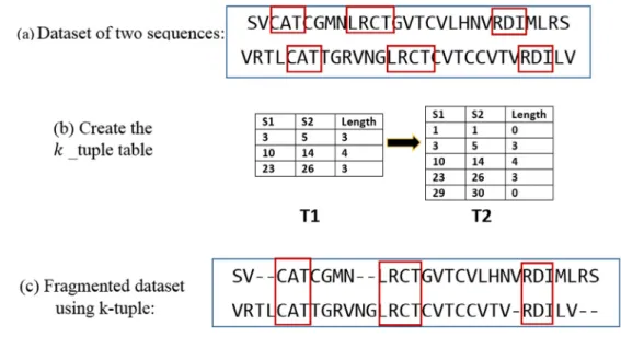
5.1. Fragmentation: table ofk-tuples
It is worth noting that PSO is performing well with short sequences (Xu and Chen, 2009; Long et al., 2009a, 2009b). A fragmentation technique is used to shorten the sequences of the datasets. Additionally, if one fragment is mis-aligned, this will not affect the other fragments. Fragmentation depends on searching for conserved regions (also called motifs or blocks) and aligning them, and then aligning the regions between these blocks to make a complete alignment. The fragmentation tech-nique used here isk-tuple. Fragmentation based onk-tuple or
k-word searches for a word of lengthk. This technique is pre-viously used in one of the oldest and fastest pairwise alignment methods: FASTA (Lipman and Pearson, 1985). Due to its sim-plicity and speed, thek-tuple could be enough in molecular phylogeny and taxonomy without the need for alignment in the future (Zuo et al., 2014). As the word length (thekvalue) increases, the accuracy of the match between the two words also increases. The k-tuple can also have a number of mismatches that don’t exceed a value D (Fig. 1), where D mutations give non-negative score in the substitution matrix.
In this case, these characters are not matched but they have a degree of similarity in their chemical structure. This -tuple technique with mutations is called Wu–Manber (Wu and Manber, 1992).
To find a word of lengthkin the dataset ofnsequences, one of thesensequences is assumed to be a query. Everyk-tuple of the query sequence is scanned with all then1 left sequences. If this word is found in all sequences, the positions of this word in all sequences are inserted into a table. This step is repeated for (Lk+ 1)k-tuples for the query of length L.
After the table has been created, and an overall check has been done to make sure that there is no conflict, two more rows must be added. As illustrated in the example inFig. 2, all matched words of k¼3 andD¼0 are gathered in table T1. The first and the last columns are added, which contain the index of the first, and the last character in every sequence as shown in tableT2. The aim of this table is to find thek-tuple words and connect between k-tuple search method and PSO. The PSO will take every two successive rows and deal with the segments in-between. Adding the first and the last two in the table will let PSO deal with the first and the last two fragments. Every time, PSO will deal with one fragment. To get the boundaries of the ith fragment for the jth sequence, every two successive rowsði;iþ1Þ in the tableT2should be considered following the equation:
Boundaryðj;iÞ ¼ ½tableði;jÞ þtableði;nþ1Þ
:½tableðiþ1;jÞ 1 ð9Þ wheretableði;nþ1Þindicates thek-tuple length to let the PSO start taking the fragment after thek-tuple ended. The aligned parts by thek-tuple method are not included in the PSO calcu-lation and may be misaligned if the particle is trapped in local optima.
5.2. Alignment: PSO 5.2.1. Particle creation
In the alignment problem, we need to find the best location of gaps which will be added. So, particles here will carry the posi-tions of these gaps in all sequences of the entered dataset. The number of dimensions for the particle will be equal to the num-ber of gaps needed to be inserted to the sequences.Fig. 3gives an example of a dataset of sequences filled with gaps.
In the example inFig. 3, a particlemhere is represented as:
m= [3, 8, 10, 1, 6, 9, 10] that carries the positions of gaps in the dataset. Another variable lis needed here to show in which sequence in the dataset the gaps will be added. Simply,lwill carry a number of gaps that will be added in each sequence. To get the starting, and the ending positions of the gaps from the particlemfor sequencejusing matrixl, next equations are used:
Figure 1 Match of two words of word lengthk= 8 andD= 3 mutations. Depending on pam250 matrix, score (V, L) = +2, score (T, A) = +1, and score (V, I) = +4.
posstartðjÞ ¼X j1 I¼0 lþ1 ð10Þ posendðjÞ ¼X j1 I¼0 lþlðjÞ þ1 ð11Þ
And so, gaps will be added to sequencejare:
gapsðjÞ ¼mðposstart:posendÞ ð12Þ The values of the gaps should be controlled by the length of the alignment (inFig. 3), som matrix should contain values <11.
5.2.2. Local-PSO
The basic PSO discussed in the previous section is called global PSO, as all particles in the swarm follows only one particle, the one which gets the best score value. Dependency of all particles on only one particle in updating global best term causes fast convergence. If thegbestis trapped, that mostly causes trap-ping of all other particles. One famous variant of PSO is local-PSO (Eberhart et al., 1996). Its main benefit over global-PSO is to keep the system divergent from trapping in local minima/maxima. Here, the swarm is divided into many sub-swarms, such that every particle calculates its local best value (instead of global best one) by finding the best positions of gaps which give the best score in the sub-swarm.
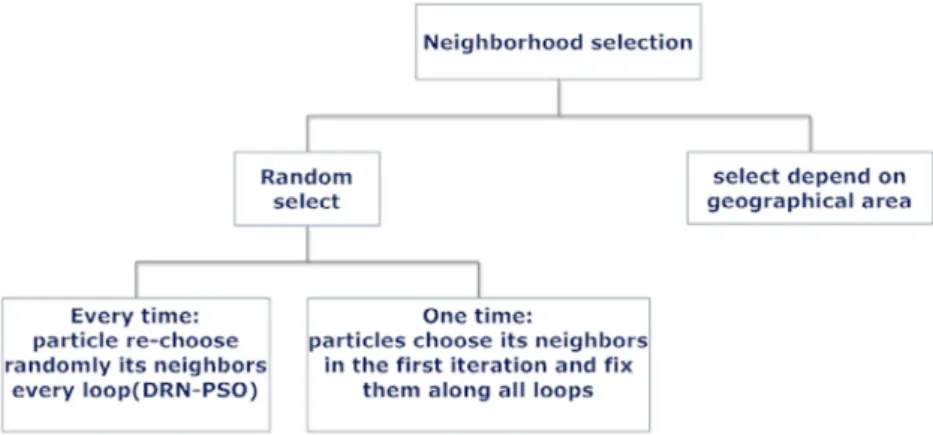
In local-PSO, every particle can choose its neighbours according to geographical area (or for alignment problem, it can selects particles of near scores), or randomly. In this paper,
particles follow randomly chosen method. As illustrated in Fig. 4, random selection for neighbourhood can be only one time or every loop. The paper follows the selection of new neighbours every loop of DRN-PSO. It presents a form of dynamic random neighbourhood, which enables each particle to change its neighbourhood during searching for the optimal solution as shown inFig. 5. This feature helps in increasing the swarm diversity (El-Hosseini et al., 2014). When the size of gbestmatrix in Eq.(5)is equal to the size of one particle only, the size oflbesthere will be equal to the size of the swarm. That lets Eq.(5)transform to Eq.(13):
vtmd¼wt:vmdt1þ ½c1:r1:ðpbestmdx t1 mdÞ þ ½c2:r2:ðlbestmdx t1 mdÞ ð13Þ
5.2.3. Best particle mutation
Every iteration of the best particle mutation method, the best particlegbestis selected to be mutated. After mutation is done, the score is calculated and compared with the one before muta-tion. If the particle after mutation gives a higher score, then keep it and update the score value in the scoring matrix (Long et al., 2009b). The algorithm of the best particle muta-tion is illustrated inFig. 6.
5.2.4. Two-layer PSO (TLPSO)
TLPSO consists of two layers. The first layer contains R swarms as shown inFig. 7, where all particles in one swarm are communicating with themselves, using a specified scoring function to get the optimal (or semi-optimal) solution for the problem. Every swarm in the first layer producesgbestas an output, so for R swarm, we can get Rgbestparticles. These R particles will create the swarm in the second layer. Finally, onegbestparticle (Gbest L2) will be resulted from the second layer.
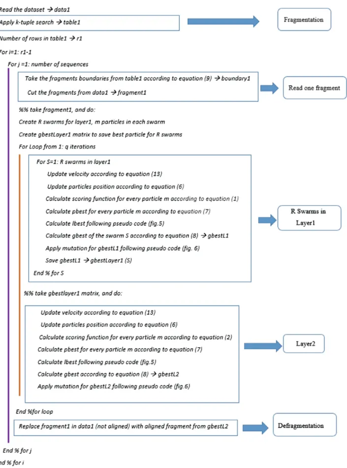
All swarms in the first layer will use the CS scoring function mentioned in Eq.(1), and the swarm in the second layer will depend on the SOP scoring function mentioned in Eq. (2). The pseudo code for FTLPSO is shown inFig. 8.
Figure 2 Example illustrates how the table linking between fragmentation and PSO is created.
Figure 3 Numerical example on how a particle of gap positions is created.mis a particle, andlis a matrix helping the particle to decide to which sequence the gap belongs.
6. Numerical results
According to the scoring functions: the scoring matrix used is PAM 250, and the gap penalty used is affine gap penalty with a gap open penaltygo=10, gap extension penaltyge=0.3,
and gap-gap penalty = 0. Concerningk-tuple search: the value ofkis chosen to be =8, with maximum number of mutations D= 3, as a suitable selection for the tested datasets, which is not too long that thek-tuple method can’t find it, nor too short which causes conflicts (Lassmann and Sonnhammer, 2005).
According to the PSO: The number of neighbourhoods for local PSO = 3, and best particle mutation is considered in every iteration. The values of acceleration coefficients c1 and
c2 arec1¼c2 = 1.49618 (Eberhart and Shi, 2000). The veloc-ity matrixvis bounded between two values (vmin; vmax) accord-ing to next equations:
vmax¼h ðxmaxðdÞ xminðdÞÞ; vmin¼ vmax ð14Þ v¼ vmax if vPvmax vmin if v<vmin ð15Þ wherexmax ðdÞ andx min
ðdÞ are the maximum and minimum positions in thedth dimension, andhis a parameter defined by user to control steps (Clerc and Kennedy, 2002). Here,his set to be =0.08 of the sequence length (AL).
Further, w is exponentially decreased according to equation:
w¼ wowf expðt=tmaxÞ
ð16Þ
Figure 4 Simple classification for selecting neighbourhood in PSO.
Figure 5 DRN-PSO algorithm.
Figure 6 Best particle mutation.
wheretis the current iteration number,tmax is the maximum number of iterations, and,wo; wf are the two boundaries of
w, withwo= 0.9, andwf= 0.4.
For two layers: number of swarms of the first layer R = 10, with 10 particles in each swarm, and the best 10 particles in layer1 will create the swarm in layer2.
The suggested algorithm has been implemented using MATLAB Ver. 8.2.0.701 (R2013b). The algorithm is applied on some Balibase (Bahr et al., 2001) benchmark datasets of dif-ferent alignment lengths, and compared with five famous MSA tools: CLUSTAL Omega, CLUSTAL W2, TCOFFEE,
KALIGN, and DIALIGN-PFAM (www.ebi.ac.uk; www.
clustal.org; http://dialign-pfam). The comparative analysis with these tools is presented in Section6.1. Next, Section6.2 gives an answer for why the used parameters have been set as they are. The parameters of the velocity update equation (Eq. (13)), and sum of pair score (SOP) equation (Eq. (4)) are studied. In the numerical study for each parameter, only the value of the studied parameter is changed, and the others are kept fixed according to their values mentioned above.
6.1. Comparative analysis
Fig. 9compares the results of standard PSO, TLPSO without fragmentation, and TLPSO with fragmentation (FTLPSO). The datasets are sorted according to their lengths. The figure represents that the standard PSO and the TLPSO have the ability to deal with short sequences. That appears in the first sequence (1fmb) where the SOP scores for standard PSO, TLPSO and FTLPSO are very close to each other. The stan-dard PSO fails to do alignment for the rest of the datasets. TLPSO overcomes the standard PSO. However, it also gave poorer results, and failed to reach the optimal solution.
Figure 9 Compare the results of standard, two layers before and after fragmentation (standard PSO vs TLPSO vs FTLPSO).
FTLPSO succeeded to reach optimal (or semi-optimal) solu-tions, and overcome both standard PSO and TLPSO.
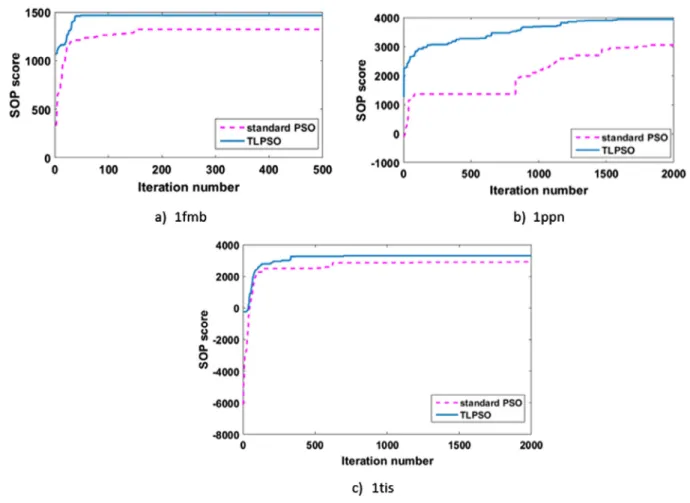
Fig. 10 gives more details regarding the performance of standard PSO, and TLPSO for 3 datasets. For the shortest, and simplest dataset, 1fmb,Fig. 10a shows how the standard PSO reached a semi-optimal solution. However, TLPSO was able to reach the optimal solution, and with less numbers of iterations. With the increase in dataset length, and complexity, particles with 1ppn dataset tried to achieve good solution along 2000 iterations. TLPSO outperformed standard PSO. However, system couldn’t reach the optimal solution. It is worth to mention the role of best-particle mutation, which helps the system to move again after it has trapped in a local minima, as it is obvious at standard PSO in (Fig. 10b). 1tis suf-fered from an early trapping in local minima although TLPSO outrun standard PSO.
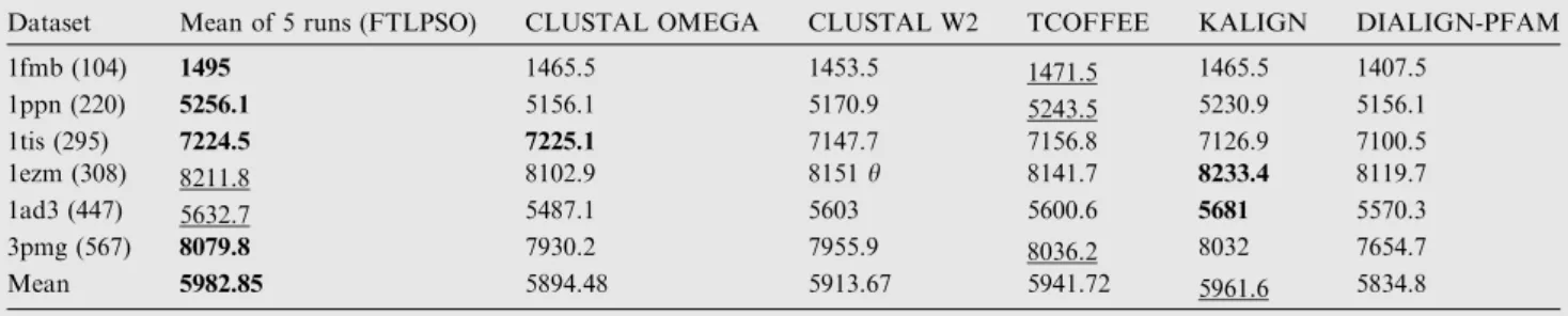
The results in Table 1 shows the ability of the proposed method to align long sequences, and the PSO is not affected with the length of the datasets. That is clearly seen in (3pmg), the longest tested dataset, that the FTLPSO over-comes the other MSA tools. That proves that the FTLPSO is the best tool which tries to keep the scores high in all the tested datasets. But for the other tools, if they get a high score with one dataset, it may fall in the other. The average score for the tested datasets inFig. 11also shows the success of the pro-posed method. That is because:
(1) The fragmentation gives the ability to the swarm to search for the optimal solution within a smaller and bounded search space.
(2) One fragment will contain less number of local optimal points, which helps the particle to face less numbers of local optimal points.
(3) For each fragment, the swarm will concentrate on find-ing the optimal solution by dealfind-ing with less number of gaps, which should be added in this fragment.
(4) If the PSO can’t find the optimal solution in one frag-ment, the other fragments will not be affected, and the overall score will remain high.
Besides the role of fragmentation process, the high perfor-mance of PSO lies in:
(1) The PSO does not discriminate one sequence over another, and it is one of the most important benefits for PSO as an iterative tool, compared to other progres-sive tools.
(2) The cooperation between particles with each other’s to reach the optimal point of the highest score.
(3) Local PSO increases the swarm diversity, and lets the particles explore more points in the search space. (4) Mutation which is applied on the gbest particle also
gives help if thegbesthas trapped in a local optima. Figs. 12 and 13give two examples to show the performance of the PSO on two fragments from 1ezm and 1ppn datasets. The selected fragment from 1ezm is of length 44, and 1ppn fragment is of length 104. For each fragment, every swarm in the first layer and the swarm in the second layer contain 10 particles, and each swarm runs for 100 iterations. For each fragment, the 10 swarms in the first layer run, and the CS score given by the best particle in layer 1 every iteration is presented in (12-a, 13-a). Figs.12b and13b show the progress of the swarm in the second layer. Rate of convergence for both layers have been normalized in (12-c, 13c) to show the effectiveness of the best particles from swarms in the first layer on the second layer’s swarm.
6.2. Parametric study
This section starts with a study for parameters in PSO velocity update equation, with focus on two parameters (velocity clamping, and inertia weight), in Section6.2.1. In Section6.2.2,
Table 1 SOP score results for FTLPSO compared with other five MSA tools. The left column contains list of datasets, and the length of the longest sequence is mentioned in brackets. The highest score is in bold, and the second is underlined.
Dataset Mean of 5 runs (FTLPSO) CLUSTAL OMEGA CLUSTAL W2 TCOFFEE KALIGN DIALIGN-PFAM
1fmb (104) 1495 1465.5 1453.5 1471.5 1465.5 1407.5 1ppn (220) 5256.1 5156.1 5170.9 5243.5 5230.9 5156.1 1tis (295) 7224.5 7225.1 7147.7 7156.8 7126.9 7100.5 1ezm (308) 8211.8 8102.9 8151h 8141.7 8233.4 8119.7 1ad3 (447) 5632.7 5487.1 5603 5600.6 5681 5570.3 3pmg (567) 8079.8 7930.2 7955.9 8036.2 8032 7654.7 Mean 5982.85 5894.48 5913.67 5941.72 5961.6 5834.8
the effectiveness of changing parameters in objective functions is also studied.
6.2.1. PSO parametric study: exploration, and exploitation
PSO, as an optimization technique, is based mainly on two concepts: Exploration, and Exploitation. Exploration is to search within the search space for new optimal solution in the places which have not been visited before. Exploitation is to search for better solution in the places that have been already visited before. Exploration and exploitation are oppo-site, as increasing exploration will limit the exploitation. Unbalancing between these two concepts may lead the parti-cles to trap in local optima (Chen, and Montgomery, 2013). To achieve good balancing, and avoid premature convergence towards a local optimum, some choices should be decided well, including (Ahmed and Glasgow, 2012):
a- Selection for the suitable values of acceleration coeffi-cient (c1,c2).
b- Limiting the particles velocity (velocity clamping). c- Good selection for inertia weight value.
6.2.1.1. Acceleration coefficients. Acceleration coefficients
c1;c2 define the ratio of dependency for every particle m in its decision for next position (x) on its best position reached (pbest) and the globally best position ðgbestÞ, respectively, where:
- Ifc1 >c2: it means that particlemwill be more biased to its historical best position pbest, to keep diversity of the swarm.
- Ifc1 <c2: it means that particlemwill be more biased to the global best positiongbest, which helps fast convergence of the swarm (Zhan et al., 2009).
Some experiments by Kennedy (1998) on some typical applications suggest the values of acceleration coefficientsc1 andc2 to be in the range [0, 4], for achieving more control on the search process, where: c1+c264. Further
experi-ments found the best values for c1, c2 to be:
c1¼c2 = 1.49618 (Eberhart and Shi, 2000).
6.2.1.2. Velocity.Velocityvdepends on the difference between the current position of the particle and its previous best posi-tion pbest, seen in the second (called cognitive) term of Eq. (13), and the difference between the current position of the particle x and its best position reached by the swarmgbest, seen in the third (social) term of the same equation. So, ini-tially, the large difference at the beginning of the iterations leads to larger velocity and more trends towards exploration. As iterations increase, the velocity h will be decreased with more trends towards exploitation (Chen and Montgomery, 2013).
In the initial iterations, if the current positionxis very large than bothpbestandgbest(xpbest&xgbest), that makes the velocity to be largely ve. In contrast, If the current
positionxis smaller than bothpbestandgbest(xpbest&
xgbest), that makes the velocity to be largely +ve. These two large values in velocity may lead to what is called ‘‘particle explosion”. That is due to control loss of the velocity magni-tude (|v|) which makes the particles leave the search space due to huge steps. To control this problem, velocity clamping is a better solution, which is mentioned in Eqs.(14) and (15). The parameterhin Eq.(14)takes values between [0, 1]. Ifh is large (near to 1), the velocity will be less-controlled, which will lead to particle explosion. Decreasing the value ofhwill lead to more control for the particles. However, if the h is set to be very small, that will lead the particle to move very slowly. The slow movement of particles (gaps) allows to explore the search space efficiently, but it takes a long time.
Five values of h are run on six Balibase benchmarks. These values are 0.008, 0.03, 0.08, 0.3, and 0.8. Results in Table 2 and Fig. 14 show that the velocity clamping with (h= 0.08) gave the best score. As increase in the h value than 0.08, or decreasing it, the scores get worse. That is because while increasing the value of h, the system moves towards throwing the gaps at the boundaries of the sequences, and then the system will be trapped. While decreasing the h value, the gaps move very slowly, and the
Figure 13 Results of running 100 iterations using 10 particles on 1ppn fragment of length 104.
Table 2 SOP scores for velocity clamping with different h values. Bold font refer to maximum score for each dataset.
Dataset h= 0.8 h= 0.3 h= 0.08 h= 0.03 h= 0.008 1fmb 1460 1495 1495 1495 1323.4 1ppn 5035.5 5224.9 5256.1 4886.3 4298.9 1tis 6450.4 7058.7 7224.5 6676 4994.7 1ezm 8077.1 8173.0 8211.8 7283.3 6814.9 1ad3 5373 5409.4 5632.7 5429.6 4975.3 3pmg 7261.6 7856.7 8079.8 7909.2 7081.4
Figure 14 Alignment scores of velocity clamping using different
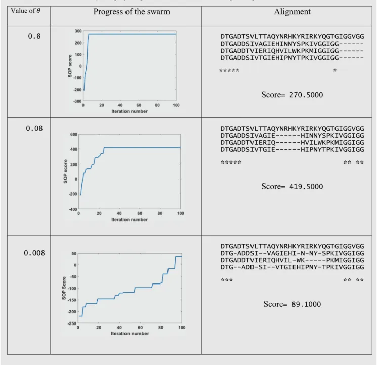
swarm takes much more time to converge. More illustrated example is seen in Table 3. Table 3 gives results for the alignment of dataset DS1 (which is given in Fig. 15) using three values of h (0.8, 0.08, and 0.008). At h= 0.8, gaps are being quickly thrown to the boundaries of the search space. By iteration 5, the system has been trapped. At
h= 0.08, the system reached the optimal solution after a few number of iterations (around 25 iterations). With a very small number of h= 0.008, positions of particles are updated very slowly, as by iteration 100, the best particle score was only 89.1. Truly, this system can reach the opti-mal solution. However, it will need more number of iterations.
Table 3 Effectiveness of velocity clamping using different values ofhon the alignment process.
Figure 15 Two small datasets: DS1, DS2, that will be used in parameters study.
6.2.1.3. Inertia weight.Inertia weight,w, introduced to acceler-ate the convergence speed of the PSO. It is another way to con-trol the velocity. Probabilities ofwcan be classified to:
– IfwP1: the velocity step will be big, and it is hard for the particle to update its direction.
– If 0<w<1: it means only a small percentage of the previ-ous velocityvt1 is kept for calculation of the new velocity vt, with quick ability for particle to change its direction.
– Ifw¼0: the first term in Eq.(13)will be deleted, and so, the second and third terms will be equal to zero when calculat-ing the new velocity of thegbestparticle, and so, the particle will not be updated, asgbest¼pbest¼x.
Changing inertia weight has been tested on many optimiza-tion problems and proves its superiority (Kumar et al., 2008). The value ofwcan be changed by either increasing or decreas-ing its value every iteration. However, dynamically changdecreas-ing the velocity by decreasing it is better in order to control the balancing between exploration and exploitation (as to start with big to increase exploration, and decrease it till be very small at the end of searching process to increase exploitation). Three weight schemes are tested in this study, which are: decreasing linearly, decreasing nonlinearly, and decreasing exponentially. Exponentially decreased w is previously men-tioned in Eq. (16). Decreasing w linearly follows the next equations:
step¼wowf
tmax ð17Þ
w¼wo ðsteptÞ ð18Þ
And nonlinearly decreased value of wfollows Eq.(19) as follows:
w¼wfþ wowf t
ð19Þ In this experiment, w is decreased from wo= 0.9, to
wf= 0.4 for all three weighting schemes.
Table 4andFig. 16show that exponentially decreasedw
was able to reach higher scores than the others two schemes. Only linearly decreased scheme won the exponentially decreased scheme in one dataset with a very little difference.
6.2.2. Objective functions parametric study
In this paper, two scoring functions are used. The first is (CS) score (Eq.(1)), which doesn’t contain parameter to be tuned. So, this section will focus on the second objective function (SOP), especially on the selection of gap penalty scores.
There are different conventions regarding the gap penalty such as linear gap penalty, and affine gap penalty. In linear gap penalty, each gap is given a penalty such that all gaps are equal in punishment value either this gap is an open of the gap series‘, or not. This makes no control on the place of the gaps. However, biologically, the possibility of having a single long gap‘ in the protein sequence is more likely to occur than the multiple small series of gaps (Gotoh, 1983). That is because if a deletion for an amino acid is created once, it is easy to be extended. For that reason, this paper used the affine gap penalty (Eq.(4)) generated byGotoh (1983).
Table 4 SOP scores for different weight schemes. Bold font refer to maximum score for each dataset.
Dataset Linearly decreased (0.9:0.4) Nonlinearly decreased (0.9:0.4) Exponentially decreased (0.9:0.4) 1fmb 1467.8 1407.7 1495 1ppn 5245.9 4937.3 5256.1 1tis 6994.7 6292.5 7224.5 1ezm 8106.8 7737.3 8211.8 1ad3 5549 5399.7 5632.7 3pmg 8089.9 7471.7 8079.8
Figure 16 Alignment scores of different weight schemes.
Figure 17 Optimal alignment on DS1 using different gap open penalty scores.
Figure 18 Optimal alignment on DS2 using different gap extension penalty scores.
Increasing the value of gap open penaltygo will lead to a reduction in the numbers of opening gaps, and the system will move towards increasing the length of a gap‘. Dataset DS1 (shown inFig. 15) is aligned three times using different gap open penalty values (2,6, and10), as inFig. 17. Although a low value of a gap open penalty may lead to more matches, it is in contrary to the biological information. Biologically, the probability that the amino acid R(in bold) was H, and has been mutated is more likely to happen. Also, it is the case with (V) in bold as it once was (I) and has been mutated. That is why this paper used a gap open penaltygoof10.
According to gap extension penaltyge, its value affects the number of gaps in the alignment. Dataset DS2 (inFig. 15) is aligned using a fixedgo, with different values. As shown in Fig. 18, when for examplegeis set to be3, the relatively high value ofgeforced the system to use more numbers of gaps, and forbade the system from achieving more matches. However, with a low value of 1, more gaps were added, with more matches.
7. Conclusion
This paper proposed FTLPSO algorithm as a contribution for solving the MSA problem. The algorithm has two main steps: the first is fragmentation of long sequences, and the second is aligning each fragment alone using two-layer PSO (TLPSO) structure. Fragmentation helps the PSO to deal with short sequences. TLPSO is a good selection for solving MSA as unconstrained problems. Solving MSA problem requires max-imization of column score (CS), as maximizing sum of pair score (SOP). The first layer in TLPSO structure contains a number of swarms, which deals with the CS scoring function. The swarm in the second layer is dealing with SOP scoring function. In every swarm, local PSO and best particle mutation are applied to keep particles far from trapping in a local optima as possible. FTLPSO is run on 6 datasets from balibase reference, and the results are compared with five state-of-the-art tools: CLUSTAL Omega, CLUSTAL W2, TCOFFEE, KALIGN, and DIALIGN-PFAM. FTLPSO overcame other tools and could keep the score high in all tested datasets. It also achieved the best average score among them. After com-paring the proposed method with other tools, a parametric study is applied which proofs the efficiency of the used values in the updating equation for PSO as in the objective function used.
As a future path of this work is to focus on studying the efficiency of different fragmentation techniques instead ofk -tuple, decreasing the memory usage, CPU usage, and increas-ing the processincreas-ing time are the main interest as future works. References
Agrawal, Ankit, Huang, Xiaoqiu, 2009. PSIBLAST_PairwiseStatSig: reordering PSI-BLAST hits using pairwise statistical significance. Bioinformatics 25 (8), 1082–1083. http://dx.doi.org/10.1093/bioin-formatics/btp089.
Ahmed, Hazem, Glasgow, Janice, 2012. Swarm Intelligence: Concepts, Models and Applications. Technical Report, School of Computing, Queen’s University.
Al Ait, L., Yamak, Z., Morgenstern, B., 2013. DIALIGN at GOBICS– multiple sequence alignment using various sources of external information. Nucl. Acids Res. 41, W3–W7.
Arulmani, K., Guru Prasad, M., Hariharan, R., Sivasankaran, N., 2012. A refined MSAPSO algorithm for improving alignment score. Res. J. Appl. Sci., Eng. Technol. 4 (21), 4404–4407. Bahr, A., Thompson, J.D., Thierry, J.-C., Poch, O., 2001. BAliBASE
(Benchmark Alignment dataBASE): enhancements for repeats, transmembrane sequences and circular permutations. Nucl. Acids Res. 29 (1), 323–326.http://dx.doi.org/10.1093/nar/29.1.323.
Botta, Marco, Negro, Guido, 2010. Multiple sequence alignment with genetic algorithms. Comput. Intell. Meth. Bioinf. Biostat. 6160, 206–214.
Chen, C.C., 2011. Two-layer particle swarm optimization for uncon-strained optimization problems. Appl. Soft Comput. 11, 295–304. Chen, S., Montgomery, J., 2013. Particle Swarm Optimization with Threshold Convergence. Evolutionary Computation (CEC), 2013 IEEE Congress, pp. 510–516. ISBN: 978-1-4799-0452-5.
Clerc, M., Kennedy, J., 2002. The particle swarm -explosion, stability, and convergence in a multidimensional complex space. IEEE Trans. Evol. Comput. 6 (1), 58–73.
Cohen, J., 2004. Bioinformatics—an introduction for computer scientists. ACM Comput. Surv. 36 (2), 122–158.http://dx.doi.org/ 10.1145/1031120.1031122.
Das, S., Abraham, A., Konar, A., 2008. Swarm intelligence algorithms in bioinformatics. Stud. Comput. Intell. 94, 113–147.
Di Francesco, V., Garnier, J., Munson, P.J., 1996. Improving protein secondary structure prediction with aligned homologous sequences. Protein Sci. 5 (1), 106–113.http://dx.doi.org/10.1002/pro.5560050113.
Do, C., Mahabhashyam, M., Brudno, M., Batzoglou, S., 2005. ProbCons: probabilistic consistency based multiple sequence alignment. Genome Res. 15, 330–340.
Eberhart, R., Shi, Y., 2000. Comparing inertia weights and constric-tion factors in particle swarm optimizaconstric-tion. Evoluconstric-tionary Compu-tation, Proceedings of the 2000 Congress, vol. 1, pp. 84–88.
Eberhart, R., Simpson, P., Dobbins, R., 1996. Computational Intel-ligence-PC Tools. Academic Press Professional Inc, ISBN 0-12-228630-8.
Edgar, R.C., 2004. MUSCLE: multiple sequence alignment with high accuracy and high throughput. Nucl. Acids Res. 32, 1792–1797.
El-Hosseini, M.A., El-Sehiemy, R.A., Haikal, A.Y., 2014. Multiob-jective optimization algorithm for secure economical/emission dispatch problems. J. Eng. Appl. Sci., Faculty Eng., Cairo University 61 (1), 83–103.
Finn, R.D., Tate, J., Mistry, J., Coggill, P.C., Sammut, S.J., et al, 2008. The Pfam protein families database. Nucl. Acids Res. 36, 281–288. Gotoh, O., 1983. An improved algorithm for matching biological sequences. J. Mol. Biol. 162 (3), 705–708. http://dx.doi.org/ 10.1016/0022-2836(82)90398-9.
Jagadamba, P.V.S.L., Babu, M.S.P., Rao, A.A., Rao, P.K.S., 2011. An improved algorithm for multiple sequence alignment using particle swarm optimization. In: Proceedings of IEEE Second International Conference on Software Engineering and Service Science, pp. 544–547. doi: 10.1109/ICSESS.2011.5982374.
Katoh, Kazutaka, Standley, Daron M., 2016. A simple method to control over-alignment in the MAFFT multiple sequence alignment program. Bioinformatics, doi:0.1093/bioinformatics/btw108.
Katoh, K., Misawa, K., Kuma, K., Miyata, T., 2002. MAFFT: a novel method for rapid multiple sequence alignment based on fast Fourier transform. Nucl. Acids Res. 30, 3059–3066.
Kennedy, J., 1998. The behaviour of particles. In: Proceedings of the 7th International Conference on Evolutionary Programming VII, vol. 1447. Springer-Verlag, London, UK, pp. 579–589.
Kennedy, J., Eberhart, R., 1995. Particle Swarm Optimization. IEEE Int. Conf. Neural Netw. 4, 1942–1948.
Kim, J., Pramanik, S., Chung, M.J., 1994. Multiple sequence align-ment using simulated annealing. Comput. Appl. Biosci. 10 (4), 419– 426.
Kiranyaz, S., Ince, T., Yildirim, A., Gabbouj, M., 2009. Multi-dimensional particle swarm optimization for dynamic clustering. EUROCON, IEEE 2009, 1398–1405.
Kumar, Ganesh, Mohagheghi, Salman, Hernandez, Jean-Carlos, delValle, Yamille, 2008. Particle Swarm Optimization: Basic Concepts, Variants and Applications in Power Systems. IEEE, pp. 171–195.
Lalwani, Soniya, Kumar, Rajesh, Gupta, Nilama, 2013a. A review on particle swarm optimization variants and their applications to multiple sequence alignment. J. Appl. Math. Bioinform. 3 (2), 87–124.
Lalwani, Soniya, Kumar, Rajesh, Gupta, Nilama, 2013b. A study on inertia weight schemes with modified particle swarm optimization algorithm for multiple sequence alignment. In: International Con-ference on Contemporary Computing (IC3). IEEE, pp. 283–288.
Lalwani, Soniya, Kumar, Rajesh, Gupta, Nilama, 2015. A novel two-level particle swarm optimization approach for efficient multiple sequence alignment. Memetic Comput., Springer 7 (2), 119–133.
Larkin, M.A., Blackshields, G., Brown, N.P., Chenna, R., McGetti-gan, P.A., McWilliam, H., Valentin, F., Wallace, I.M., Wilm, A., Lopez, R., Thompson, J.D., Gibson, T.J., Higgins, D.G., 2007. Clustal W and Clustal X version 2. Bioinformatics 23 (21), 2947– 2948.
Lassmann, T., Sonnhammer, E.L.L., 2005. Kalign-an accurate and fast multiple sequence alignment algorithm. BMC Bioinform. 6 (298).
Lipman, D.J., Pearson, W.R., 1985. Rapid and sensitive protein similarity searches. Science 227, 1435–1441.
Long, Hai-Xia, Xu, Wen-Bo, Sun, Jun, Ji, Wen-Juan, 2009a. Multiple sequence alignment based on a binary particle swarm optimization algorithm. IEEE Fifth International Conference on Natural Computation. vol. 3, pp. 265–269.
Long, Hai-Xia, Xu, Wen-Bo, Sun, Jun, 2009b. Binary particle swarm optimization algorithm with mutation for multiple sequence alignment. Riv. Biol. 102 (1), 75–94.
Morgenstern, B., Dress, A., Werner, T., 1996. Multiple DNA and protein sequence alignment based on segment-to-segment compar-ison. Proc. Natl. Acad. Sci. U. S. A. 93, 12098–12103.
Morgenstern, B., Prohaska, S.J., Po¨hler, D., Stadler, P.F., 2006. Multiple sequence alignment with user-defined anchor points. Algorithms Mol. Biol. 1 (6).
Mount, D.W., 2004. Bioinformatics Sequence and Genome Analysis, second ed. Cold Spring Harbor Laboratory Press.
Needleman, S.B., Wunsch, C.D., 1970. A general method applicable to the search for similarity in the amino acid sequences of two proteins. J. Mol. Biol. 48, 443–453.
Notredame, C., Higgins, D.G., 1996. SAGA: sequence alignment by genetic algorithm. Nucl. Acids Res. 24 (8), 1515–1524.
Notredame, C., Higgins, D.G., Heringa, J., 2000. T-COFFEE: a novel method for fast and accurate multiple sequence alignment. J. Mol. Biol. 302 (1), 205–217.
Pais, F.S., Ruy Pde, C., Oliveira, G., Coimbra, R.S., 2014. Assessing the efficiency of multiple sequence alignment programs. Algorithms Mol. Biol. 9 (4).
Pankaj, S., Pankaj, S.P., 2013. A DNA sequential alignment using dynamic programming and PSO. Int. J. Eng. Innovative Technol. (IJEIT) 2 (11), 257–264.
Roshan, U., Livesay, D.R., 2006. Probalign: multiple sequence alignment using partition function posterior probabilities. Bioin-formatics 22, 2715–2721.
Sierk, Michael L., Smoot, Michael E., Bass, Ellen J., Pearson, William R., 2010. Improving pairwise sequence alignment accuracy using near-optimal protein sequence alignments. BMC Bioinform. 11 (146).http://dx.doi.org/10.1186/1471-2105-11-146.
Sievers, F., Wilm, A., Dineen, D.G., Gibson, T.J., Karplus, K., Li, W., Lopez, R., McWilliam, H., Remmert, M., So¨ding, J., Thompson, J. D., Higgins, D., 2011. Fast, scalable generation of high-quality protein multiple sequence alignments using clustal omega. Mol. Syst. Biol. 7.http://dx.doi.org/10.1038/msb.2011.75. Article number: 539. Smith, Temple F., Waterman, Michael S., 1981. Identification of common molecular subsequences. J. Mol. Biol. 147, 195–197.
http://dx.doi.org/10.1016/0022-2836(81)90087-5. PMID 7265238.
Subramanian, A.R., Kaufmann, M., Morgenstern, B., 2008. DIA-LIGN-TX: greedy and progressive approaches for the segment-based multiple sequence alignment. Algorithms. Mol. Biol. 3 (6).
Suresh, G., Vijayalakshmi, C., 2013. A novel approach based on approximation and heuristic methods using multiple sequence alignments. Indian J. Appl. Res. 3 (5), 36–40.
Thompson, J.D., Higgins, D.G., Gibson, T.J., 1994. CLUSTAL W: improving the sensitivity of progressive multiple sequence align-ment through sequence weighting, positions-specific gap penalties and weight matrix choice. Nucl. Acids Res. 22, 4673–4680.
Wu, S., Manber, U., 1992. Fast text searching allowing errors. Commun. ACM 35, 83–91.
Xu, Fasheng, Chen, Yuehui, 2009. A method for multiple sequence alignment based on particle swarm optimization. Emerging Intel-ligent Computing Technology and Applications. With Aspects of Artificial Intelligence, Lecture Notes in Computer Science, vol. 5755, pp. 965–973.
Zhan, Zhi-Hui, Zhang, Jun, Li, Yun, Chung, Henry Shu-Hung, 2009. Adaptive particle swarm optimization. IEEE Trans. Syst., Man, Cybern.-Part B: Cybern. 39 (6), 1362–1381.
Zuo, Guanghong, Li, Qiang, Hao, Bailin, 2014. On K-peptide length in composition vector phylogeny of prokaryotes. Comput. Biol. Chem. 53, 166–173.