Multi-Domain Adversarial Learning

UCSF

UC San Francisco Previously Published Works

Title

Multi-Domain Adversarial Learning

Permalink

https://escholarship.org/uc/item/1h640644

Authors

Schoenauer-Sebag, Alice

Heinrich, Louise

Schoenauer, Marc

et al.

Publication Date

2019

Peer reviewed

Published as a conference paper at ICLR 2019

M

ULTI

-D

OMAIN

A

DVERSARIAL

L

EARNING

Alice Schoenauer Sebag1,†

[email protected] Louise Heinrich1_, [email protected] Marc Schoenauer2_, [email protected] Michele Sebag2_, [email protected] Lani F. Wu1_, [email protected] Steven J. Altschuler1 [email protected] 1_{Department of Pharmaceutical Chemistry}

UCSF, San Francisco, CA 94158

2_{INRIA-CNRS-UPSud-UPSaclay}

TAU, U. Paris-Sud, 91405 Orsay

A

Multi-domain learning (MDL) aims at obtaining a model with minimal average risk across multiple domains. Our empirical motivation is automated microscopy data, where cultured cells are imaged after being exposed to known and unknown chemical perturbations, and each dataset displays significant experimental bias. This paper presents a multi-domain adversarial learning approach, MULANN, to leverage multiple datasets with overlapping but distinct class sets, in a semi-supervised setting. Our contributions include: i) a bound on the average- and worst-domain risk in MDL, obtained using theH-divergence; ii) a new loss to accommodate semi-supervised multi-domain learning and domain adaptation; iii) the experimental validation of the approach, improving on the state of the art on three standard image benchmarks, and a novel bioimage dataset, CELL.1

1

I

Advances in technology have enabled large scale dataset generation by life sciences laboratories. These datasets contain information about overlapping but non-identical known and unknown experi-mental conditions. A challenge is how to best leverage information across multiple datasets on the same subject, and to make discoveries that could not have been obtained from any individual dataset alone.

Transfer learning provides a formal framework for addressing this challenge, particularly crucial in cases where data acquisition is expensive and heavily impacted by experimental settings. One such field is automated microscopy, which can capture thousands of images of cultured cells after exposure to different experimental perturbations (e.g from chemical or genetic sources). A goal is to classify mechanisms by which perturbations affect cellular processes based on the similarity of cell images. In principle, it should be possible to tackle microscopy image classification as yet another visual object recognition task. However, two major challenges arise compared to mainstream visual object recognition problems (Russakovsky et al., 2015). First, biological images are heavily impacted by experimental choices, such as microscope settings and experimental reagents. Second, there is no standardized set of labeled perturbations, and datasets often contain labeled examples for a subset of possible classes only. This has limited microscopy image classification to single datasets and does not leverage the growing number of datasets collected by the life sciences community. These challenges make it desirable to learn models across many microscopy datasets, that achieve both good robustness w.r.t. experimental settings and good class coverage, all the while being robust to the fact that datasets contain samples from overlapping but distinct class sets.

†Now at the French Ministry for the Economy and Finance, 75012 Paris.

1

Code and data: github.com/AltschulerWu-Lab/MuLANN

Multi-domain learning (MDL) aims to learn a model of minimal risk from datasets drawn from distinct underlying distributions (Dredze et al., 2010), and is a particular case of transfer learning (Pan & Yang, 2010). As such, it contrasts with the so-called domain adaptation (DA) problem (Bickel et al., 2007; Ben-David et al., 2010; Ganin et al., 2016; Pan & Yang, 2010). DA aims at learning a model with minimal risk on a distribution called "target" by leveraging other distributions called "sources". Notably, most DA methods assume that target classes are identical to source classes, or a subset thereof in the case of partial DA (Cao et al., 2018; Zhang et al., 2018).

The expected benefits of MDL, compared to training a separate model on each individual dataset, are two-fold. First, MDL leverages more (labeled and unlabeled) information, allowing better generalization while accommodating the specifics of each domain (Dredze et al., 2010; Xiao et al., 2016). Thus, MDL models have a higher chance ofab initioperforming well on a new domain −a problem referred to as domain generalization (Muandet et al., 2013) or zero-shot domain adaptation (Yang & Hospedales, 2015). Second, MDL enables knowledge transfer between domains: in unsupervised and semi-supervised settings, concepts learned on one domain are applied to another, significantly reducing the need for labeled examples from the latter (Pan & Yang, 2010).

Learning a single model from samples drawn fromndistributions raises the question of available learning guarantees regarding the model error on each distribution. Kifer et al. (2004) introduced the notion ofH-divergence to measure the distance between source and target marginal distributions in DA. Ben-David et al. (2006; 2010) have shown that a finite sample estimate of this divergence can be used to bound the target risk of the learned model.

The contributions of our work are threefold. First, we extend the DA guarantees to MDL (Sec. 3.1), showing that the risk of the learned model over all considered domains is upper bounded by the oracle risk and the sum of theH-divergences between any two domains. Furthermore, an upper bound on the classifier imbalance (the difference between the individual domain risk, and the average risk over all domains) is obtained, thus bounding the worst-domain risk. Second, we propose the approach Multi-domain Learning Adversarial Neural Network(MULANN), which extends Domain Adversarial Neural Networks (DANNs) (Ganin et al., 2016) to semi-supervised DA and MDL. Relaxing the DA assumption, MULANNhandles the so-called class asymmetry issue (when each domain may contain varying numbers of labeled and unlabeled examples of a subset of all possible classes), through designing a new loss (Sec. 3.2). Finally, MULANNis empirically validated in both DA and MDL settings (Sec. 4), as it significantly outperforms the state of the art on three standard image benchmarks (Saenko et al., 2010; Le Cun et al., 1998), and a novel bioimage benchmark, CELL, where the state of the art involves extensive domain-dependent pre-processing.

Notation. LetX denote an input space andY ={1, . . . , L}a set of classes. Fori = 1, . . . , n, datasetSiis an iid sample drawn from distributionDionX × Y. The marginal distribution ofDi onX is denoted byDX

i . LetHbe a hypothesis space; for eachhinH(h:X 7→ Y) we define the risk under distributionDiasi(h) =Px,y∼Di(h(x)6=y).h

?

i (respectivelyh?) denotes the oracle hypothesis according to distributionDi(resp. with minimal total risk over all domains):

?_i =i(h?i) =min h∈Hi(h) (1) ¯ (h?) =min h∈H¯(h) =minh∈H 1 n X i i(h) (2)

In the semi-supervised setting, the label associated with an instance might be missing. In the following, "domain" and "distribution" will be used interchangeably, and the "classes of a domain" denote the classes for which labeled or unlabeled examples are available in this domain.

2

S

Machine learning classically relies on the iid setting: when training and test samples are independently drawn from the same joint distributionP(X, Y) (Vapnik, 1998). Two other settings emerged in the 1990s, "concept drift" and "covariate shift". They respectively occur when conditional data distributionsP(Y|X)and marginal data distributionsP(X)change, either continuously or abruptly, across training data or between train and test data (Shimodaira, 2000). Since then, transfer learning has come to designate methods to learn across drifting, shifting or distinct distributions, or even distinct tasks (Pratt et al., 1991; Pan & Yang, 2010). Restricting ourselves to addressing a single

Published as a conference paper at ICLR 2019

task on a common input space, we distinguish two objectives: minimizing the learning risk overall considered distributions (MDL), or overa singletarget distribution while exploiting samples from richer source(s) (DA). MDL is thus distinct from multiple source DA by their respective focus on the average risk over all distributions, versus target accuracy only. Samples from the different domains can be all, partially, or not labeled (supervised, semi-supervised and unsupervised settings). Finally, different domains can involve the same classes, or some domains can involve classes not included in other domains, referred to asclass asymmetry.

In MDL, the different domains can be taken into account by maintaining shared and domain-specific parameters (Dredze et al., 2010), or through a specific use of shared parameters. The domain-dependent use of these parameters can be learned, e.g. using domain-guided dropout (Xiao et al., 2016), or based on prior knowledge about domain semantic relationships (Yang & Hospedales, 2015). Early DA approaches leverage source examples to learn on the target domain in various ways, e.g. through reweighting source datapoints (Mansour, 2009; Huang et al., 2006; Gong et al., 2013), or defining an extended representation to learn from both source and target (Daumé III & Marcu, 2006). Other approaches proceed by aligning the source and target representations with PCA-based correlation alignment (Sun et al., 2016), or subspace alignment (Fernando et al., 2015). In the field of computer vision, a somewhat related way of mapping examples in one domain onto the other is image-to-image translation, possibly in combination with a generative adversarial network (see references in Appendix A).

Intuitively, the difficulty of DA crucially depends on the distance between source and target distribu-tion. Accordingly, a large set of DA methods proceed by reducing this distance in the original input spaceX, e.g. via importance sampling (Bickel et al., 2007) or by modifying the source representation using optimal transport (Courty et al., 2017; Damodaran et al., 2018). Another option is to map source and target samples on a latent space where they will have minimal distance. Neural networks have been intensively exploited to build such latent spaces, either through generative adversarial mechanisms (Tzeng et al., 2017; Ghifary et al., 2016), or through combining task objective with an approximation of the distance between source(s) and target. Examples of used distances include the Maximum Mean Discrepancy due to Gretton et al. (2007) (Tzeng et al., 2014; Bousmalis et al., 2016), some of its variants (Long et al., 2015; 2016), theL2contrastive divergence (Motiian et al.,

2017), the Frobenius norm of the output feature correlation matrices (Sun & Saenko, 2016), or theH-divergence (Ben-David et al., 2006; 2010; Ganin et al., 2016; Pei et al., 2018; Long et al., 2017) (more in Sec. 3). Most DA methods assume that source(s) and target contain examples from the same classes; in particular, in standard benchmarks such as OFFICE(Saenko et al., 2010), all domains contain examples from the same classes. Notable exceptions are partial DA methods, where target classes are expected to be a subset of source classes e.g. (Zhang et al., 2018; Cao et al., 2018). DA and partial DA methods share two drawbacks when applied to semi-supervised MDL with non-identical domain class sets. First, neither generic nor partial DA methods try to mitigate the impact of unlabeled samples from a class without any labeled counterparts. Second, as they focus on target performance, (partial) DA methods do not discuss the impact of extra labeled source classes on source accuracy. However, as shown in Sec. 4.3, class asymmetry can heavily impact model performance if not accounted for.

Bioinformatics is increasingly appreciating the need for domain adaptation methods (Borgwardt et al., 2006; Schweikert et al., 2008; Xu & Yang, 2011; Vallania et al., 2017). Indeed, experimentalists regularly face the issues of concept drift and covariate shift. Most biological experiments that last more than a few days are subject to technical variations between groups of samples, referred to asbatch effects. Batch effects in image-based screening data are usually tackled with specific normalization methods (Birmingham et al., 2009). More recently, work by Ando et al. (2017) applied CorAl (Sun et al., 2016) for this purpose, aligning each batch with the entire experiment. DA has been applied to image-based datasets for improving or accelerating image segmentation tasks (Becker et al., 2015; van Opbroek et al., 2015; Bermúdez-Chacón et al., 2016; Kamnitsas et al., 2017). However, to our knowledge, MDL has not yet been used in Bioimage Informatics, and this work is the first to leverage distinct microscopy screening datasets using MDL.

3

M

-D

A

L

TheH-divergence has been introduced to bound the DA risk (Ben-David et al., 2006; 2010; Ganin et al., 2016). This section extends the DA theoretical results to the MDL case (Sec. 3.1), supporting

the design of the MULANNapproach (Sec. 3.2). The reader is referred to Appendix B for formal definitions and proofs.

3.1 H-DIVERGENCE FORMDL

The distance between source and target partly governs the difficulty of DA. TheH-divergence has been introduced to define such a distance which can be empirically estimated with proven guarantees (Batu et al., 2000; Kifer et al., 2004). This divergence measures how well one can discriminate between samples from two marginals. It inspired an adversarial approach to DA (Ganin et al., 2016), through the finding of a feature space in which a binary classification loss between source and target projections is maximal, and thus theirH-divergence minimal. Furthermore, the target risk is upper-bounded by the empirical source risk, the empiricalH-divergence between source(s) and target marginals, and the oracle DA risk (Ben-David et al., 2006; 2010; Zhang et al., 2012).

Bounding the MDL loss using theH-divergence. A main difference between DA and MDL is that MDL aims to minimize the average risk over all domains while DA aims to minimize the target risk only. Considering for simplicity a binary classification MDL problem and taking inspiration from (Mansour et al., 2008; Ben-David et al., 2010), the MDL loss can be formulated as an optimal convex combination of domain risks. A straightforward extension of Ben-David et al. (2010) (Theorem 2 in Appendix B.2) establishes that the compound empirical risk is upper bounded by the sum of: i) the oracle risk on each domain; ii) a statistical learning term involving the VC dimension ofH; iii) the divergence among any two domains as measured by theirH-divergence and summed oracle risk. This result states that, assuming a representation in which domains are as indistinguishable as possible and on which every 1- and 2-domain classification task is well addressed, then there exists a model that performs well on all of them. In the 2-domain case, the bound is minimized when one minimizes the convex combination of losses in the same proportion as samples.

Bounding the worst risk. The classifier imbalance w.r.t. thei-th domain is defined as|i(h)−¯(h)|. The extent to which marginalDi can best be distinguished by a classifier from H(i.e., the H -divergence), and the intrinsic difficulty?_i of thei-th classification task, yield an upper-bound on the classifier imbalance (proof in Appendix B.3):

Proposition 1. Given an input spaceX,ndistributionsDioverX × {0,1}and hypothesis classH onX, for anyh∈ H, leti(h)(respectively¯(h)) denote the classification risk ofhw.r.t. distribution Di(resp. its average risk over allDi). The risk imbalance|i(h)−¯(h)|is upper bounded as:

|i(h)−¯(h)| ≤?i + 1 n X j ?_j+1 n X j dH(DiX,D X j ) + ∆ij (3) with∆ij =max(EDX j |h ? i(x)−h?j(x)|, EDX i |h ? i(x)−h?j(x)|)

Accordingly, every care taken to minimizeH-divergences or∆ij(e.g. using the class-wise contrastive losses (Motiian et al., 2017)) improves the above upper bound. An alternative bound of the classifier imbalance can be obtained by using theH∆H-divergence (proposition 3, and corollaries 4, 5 for the 2-domain case in Appendix).

3.2 MULANN: MULTI-DOMAIN ADVERSARIAL LEARNING

As pointed out by e.g. Pei et al. (2018), when minimizing theH-divergence between two domains, a negative transfer can occur in the case of class asymmetry, when domains involve distinct sets of classes. For instance, if a domain has unlabeled samples from a class which is not present in the other domains, both global (Ganin et al., 2016) and class-wise (Pei et al., 2018) domain alignments will likely deteriorate at least one of the domain risks by putting the unlabeled samples close to labeled ones from the same domain. A similar issue arises if a domain has no (labeled or unlabeled) samples in classes which are represented in other domains. In general, unlabeled samples are only subject to constraints from the domain discriminator, as opposed to labeled samples. Thus, in the case of class asymmetry, domain alignment will tend to shuffle unlabeled samples more than labeled ones. This limitation is addressed in MULANNby defining a new discrimination task referred to asKnown Unknown Discrimination(KUD). Let us assume that, in each domain, a fractionp? of unlabeled samples comes from extra classes, i.e. classes with no labeled samples within the domain. KUD aims at discriminating, within each domain, labeled samples from unlabeled ones that most likely belong to such extra classes. More precisely, unlabeled samples of each domain are ranked according to the entropy of their classification according to the current classifier, restricted to their domain classes.

Published as a conference paper at ICLR 2019 ' 0.0 0.3 0.5_p 0.7 1.0 0.00 0.05 0.10 0.15 0.20 0.25

Test error on MNIST-M

p =0.3 p =0.5 p =0.7 p =1 Labeled data Unlabeled data

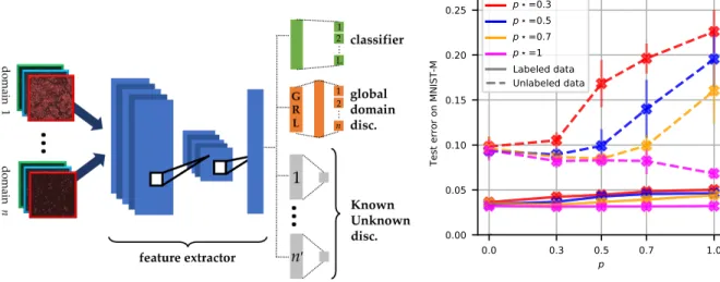
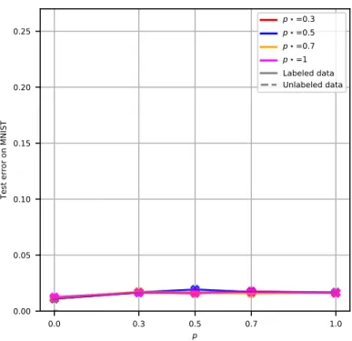
Figure 1: Left: MULANNarchitecture. GRL: gradient reversal layer from Ganin et al. (2016). Right: impact of parameterpin comparison with the groundtruthp? _{on MNIST→MNIST-M. p = 0} corresponds to DANN: no data flowed through the KUD module (see text for details).

Introducing the hyper-parameterp, the topp% examples according to this classification entropy are deemed "most likely unknown", and thus discriminated from the labeled ones of the same domain. The KUD module aims at repulsing the most likely unknown unlabeled samples from the labeled ones within each domain (Fig. 1), thus resisting the contractive effects of global domain alignment. Overall, MULANNinvolves 3+n0 interacting modules, wheren0 is the number of domains with unlabeled data. The first module is the feature extractor with parametersθf, which maps the input spaceX to some latent feature spaceΩ. 2+n0 modules are defined onΩ: the classifier module, the domain discriminator module, and then0KUD modules, with respective parametersθc,θdand

(θu,i)i. All modules are simultaneously learned by minimizing lossL(θf, θc, θd, θu):

L(θf, θc, θd, θu) = 1 n n X i=1 Li c(θf, θc)−λLid(θf, θd) + ζ n0 n0 X j=1 Lj u(θf, θu,j) (4) whereζandλare hyper-parameters,Li

c(θf, θc)is the empirical classification loss on labeled exam-ples inSi,Lid(θf, θd)is the domain discrimination loss (multi-class cross-entropy loss of classifying examples fromSi in classi), andLiu(θf, θu,i)is the KUD loss (binary cross-entropy loss of dis-criminating labelled samples fromSi from the "most likely unknown" unlabelled samples from

Si).

The loss minimization aims to find a saddle point(ˆθf,θˆy,θˆd,θˆu), achieving an equilibrium between the classification performance, the discrimination among domains (to be prevented) and the dis-crimination among labeled and some unlabeled samples within each domain (to be optimized). The sensitivity w.r.t. hyperparameterpwill be discussed in Sec. 4.3.

4

E

This section reports on the experimental validation of MULANN in DA and MDL settings on three image datasets (Sec. 4.2), prior to analyzing MULANNand investigating the impact of class asymmetry on model performances (Sec. 4.3).

4.1 IMPLEMENTATION

Datasets The DA setting considers three benchmarks: DIGITS, including the well-known MNIST and MNIST-M (Le Cun et al., 1998; Ganin et al., 2016); Synthetic road signs and German traffic sign benchmark (Chigorin et al., 2012; Stallkamp et al., 2012) and OFFICE(Saenko et al., 2010). The MDL setting considers the new CELLbenchmark, which is made of fluorescence microscopy images of cells (detailed in Appendix C). Each image contains tens to hundreds of cells that have been exposed to a given chemical compound, in three domains: California (C), Texas (T) and England (E). There are 13 classes across the three domains (Appendix, Fig. 2); a drug class is a group of compounds targeting a similar known biological process, e.g. DNA replication. Four domain shifts are considered: C↔T, T↔E, E↔C and C↔T↔E.

Baselines and hyperparameters. In all experiments, MULANNis compared to DANN (Ganin et al., 2016) and its extension MADA (Pei et al., 2018) (that involves one domain discriminator module per class rather than a single global one). For DANN, MADA and MULANN, the same pre-trained VGG-16 architecture (Simonyan & Zisserman, 2014) from Caffe (Jia et al., 2014) is used for OFFICEand CELL2; the same small convolutional network as Ganin et al. (2016) is used for DIGITS(see Appendix D.1 for details). The models are trained in Torch (Collobert et al., 2011) using stochastic gradient descent with momentum (ρ= 0.9). As in (Ganin et al., 2016), no hyper-parameter grid-search is performed for OFFICEresults - double cross-validation is used for all other benchmarks. Hyper-parameter ranges can be found in Appendix D.2.

Semi-supervised setting. For OFFICEand CELL, we follow the experimental settings from Saenko et al. (2010). A fixed number of labeled images per class is used for one of the domains in all cases (20 for Amazon, 8 for DSLR and Webcam, 10 in CELL). For the other domain, 10 labeled images per class are used for half of the classes (15 for OFFICE, 4 for CELL). For DIGITSand RoadSigns, all labeled source train data is used, whereas labeled target data is used for half of the classes only (5 for DIGITS, 22 for RoadSigns). In DA, the evaluation is performed on all target images from the unlabeled classes. In MDL, the evaluation is performed on all source and target classes (considering labeled and unlabeled samples).

Evaluation goals. A first goal is to assess MULANNperformance comparatively to the baselines. A second goal is to assess how the experimental setting impacts model performance. As domain discriminator and KUD modules can use both labeled and unlabeled images, a major question regards the impact of seeing unlabeled images during training. Two experiments are conducted to assess this impact: a) the same unlabeled images are used for training and evaluation (referred to asfully transductivesetting, noted FT) ; b) some unlabeled images are used for training, and others for evaluation (referred to asnon-fully transductivesetting, noted NFT). (The case where no unlabeled images are used during training is discarded due to poor results).

4.2 EVALUATION

DA onDIGITS, RoadSigns andOFFICE. Table 1 compares MULANNwith DANNand MADA (Sec. 4.1). Other baselines include: Learning from source and target examples with no transfer loss; Published results from (Motiian et al., 2017) (legend CCSA), that uses a contrastive loss to penalizes large (resp. small) distances between same (resp. different) classes and different domains in the feature space; Published results from (Tzeng et al., 2015), an extension of DANNthat adds a loss on target softmax values ("soft label loss"; legend Tseng15). Overall, MULANNyields the best results, significantly improving upon the former best results on the most difficult cases, i.e., D→A, A→D or W→A. As could be expected, the fully transductive results match or significantly outperform the non-fully transductive ones. Notably, MADAperforms similarly to DANNon DIGITSand RoadSigns, but worse on OFFICE; a potential explanation is that MADAis hindered as the number of classes, and thus domain discriminators, increases (respectively 10, 32 and 43 classes).

MDL onCELL. A state of the art method for fluorescence microscopy images relies on tailored approaches for quantifying changes to cell morphology (Kang et al., 2016). Objects (cells) are segmented in each image, and circa 650 shape, intensity and texture features are extracted for each object in each image. Theprofileof each image is defined as the vector of its Kolmogorov-Smirnov statistics, computed for each feature by comparing its distribution to that of the same feature from pooled negative controls of the same plate3_{. Classification in profile space is realized using linear}

discriminant analysis, followed by k-nearest neighbor (LDA+k-NN) ("Baseline P" in Table 2). As a state of the art shallow approach to MDL to be applied in profile space, CORAL (Sun et al., 2016) was chosen ("P + CORAL" in Table 2). A third baseline corresponds to fine-tuning VGG-16 without any transfer loss ("Baseline NN").

Table 2 compares DANN, MADAand MULANNto the baselines, where columns 4-7 (resp. 8-9) consider raw images (resp. the profile representations).4 _{The fact that a profile-based baseline}

generally outperforms an image-based baseline was expected, as profiles are designed to reduce the impact of experimental settings (column 4 vs. 8). The fact that standard deviations tend to be larger

2_{Complementary experiments with AlexNet (Krizhevsky et al., 2012) yield worse results, as already noted}

by (Koniusz et al., 2016).

3_{A plate contains between 96 and 384 experiments, realized the same day in exactly the same conditions.} 4

Published as a conference paper at ICLR 2019

Table 1: Classification results on target test set in the semi-supervised DA setting (average and stdev on 5 seeds or folds). Bold: results less than 1 stdev from the best in each column. See text.

Source Mnist SynSigns DSLR Amazon Webcam DSLR Webcam Amazon OFFICE

Target Mnist-M GTSRB Amazon DSLR DSLR Webcam Amazon Webcam average

Baseline 35.6 (0.6) 85.1 (1.2) 35.5 (0.5) 58.5 (1.7) 90.9 (1.8) 90.6 (0.6) 34.4 (2.7) 55.8 (1.5) 61.0 Tzeng15 - - 43.1 (0.2) 68.0 (0.5) 97.5 (0.1) 90.0 (0.2) 40.5 (0.2) 59.3 (0.6) 66.4 CCSA - - 42.6 (0.6) 70.5 (0.6) 96.2 (0.3) 90.0 (0.2) 43.6 (1.0) 63.3 (0.9) 67.8 NFT DANN 90.4 (1.1) 89.8 (1.1) 50.9 (2.4) 68.6 (4.9) 88.8 (3.2) 91.9(0.7) 48.8 (3.8) 73.0 (2.6) 70.3 MADA 89.9 (0.8) 88.7 (1.0) 44.8 (3.3) 64.0 (3.9) 88.2 (4.2) 89.1 (3.4) 44.7 (4.8) 72.2 (3.1) 67.2 MULANN 91.5 (0.4) 92.1 (1.4) 57.6(3.9) 75.8(3.7) 93.3(2.5) 89.9 (1.6) 54.9(3.9) 76.8(3.1) 74.7 FT DANN 90.6 (1.2) 86.7 (0.8) 52.2 (2.2) 77.4 (2.2) 94.6(1.2) 90.7(1.7) 53.0 (1.9) 74.3 (2.7) 73.7 MADA 91.0 (1.1) 84.8 (1.6) 51.6 (2.5) 78.8 (3.6) 91.7 (1.7) 88.8 (2.3) 53.8 (2.6) 73.5 (2.2) 73.0 MULANN 92.7 (0.6) 89.1 (1.5) 63.9(2.4) 81.7(1.7) 95.4(2.4) 89.3(2.8) 64.2(2.5) 80.8(2.7) 79.2

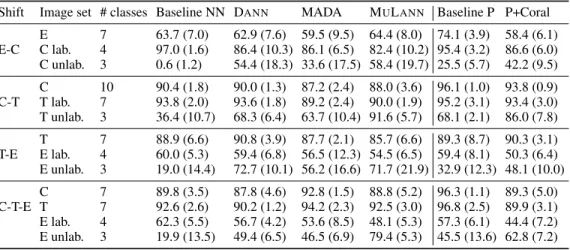
Table 2: CELLtest classification accuracy results on all domains (average and stdev on 5 folds), in the fully transductive setting (see table 5 in Appendix for non-transductive ones, and sections C.4, C.5 for details about image and class selection).

Shift Image set # classes Baseline NN DANN MADA MULANN Baseline P P+Coral

E-C E 7 63.7 (7.0) 62.9 (7.6) 59.5 (9.5) 64.4 (8.0) 74.1 (3.9) 58.4 (6.1) C lab. 4 97.0 (1.6) 86.4 (10.3) 86.1 (6.5) 82.4 (10.2) 95.4 (3.2) 86.6 (6.0) C unlab. 3 0.6 (1.2) 54.4 (18.3) 33.6 (17.5) 58.4 (19.7) 25.5 (5.7) 42.2 (9.5) C-T C 10 90.4 (1.8) 90.0 (1.3) 87.2 (2.4) 88.0 (3.6) 96.1 (1.0) 93.8 (0.9) T lab. 7 93.8 (2.0) 93.6 (1.8) 89.2 (2.4) 90.0 (1.9) 95.2 (3.1) 93.4 (3.0) T unlab. 3 36.4 (10.7) 68.3 (6.4) 63.7 (10.4) 91.6 (5.7) 68.1 (2.1) 86.0 (7.8) T-E T 7 88.9 (6.6) 90.8 (3.9) 87.7 (2.1) 85.7 (6.6) 89.3 (8.7) 90.3 (3.1) E lab. 4 60.0 (5.3) 59.4 (6.8) 56.5 (12.3) 54.5 (6.5) 59.4 (8.1) 50.3 (6.4) E unlab. 3 19.0 (14.4) 72.7 (10.1) 56.2 (16.6) 71.7 (21.9) 32.9 (12.3) 48.1 (10.0) C-T-E C 7 89.8 (3.5) 87.8 (4.6) 92.8 (1.5) 88.8 (5.2) 96.3 (1.1) 89.3 (5.0) T 7 92.6 (2.6) 90.2 (1.2) 94.2 (2.3) 92.5 (3.0) 96.8 (2.5) 89.9 (3.1) E lab. 4 62.3 (5.5) 56.7 (4.2) 53.6 (8.5) 48.1 (5.3) 57.3 (6.1) 44.4 (7.2) E unlab. 3 19.9 (13.5) 49.4 (6.5) 46.5 (6.9) 79.4 (5.3) 45.5 (13.6) 62.8 (7.2)

here than for OFFICE, RoadSigns or DIGITSis explained by a higher intra-class heterogeneity; some classes comprise images from different compounds with similar but not identical biological activity. Most interestingly, MULANNand P+CORAL both improve classification accuracy on unlabeled classes at the cost of a slighty worse classification accuracy for the labeled classes (in all cases but one). This is explained as reducing the divergence between domain marginals on the latent feature space prevents the classifier from exploiting dataset-dependent biases. Overall, MULANNand P+CORAL attain comparable results on two-domain cases, with MULANNperforming significantly better in the three-domain case. Finally, MULANNmatches or significantly outperforms DANNand MADA.

4.3 ANALYSES

Two complementary studies are conducted to investigate the impact of hyperparameterpand that of class asymmetry. The tSNE (van der Maaten & Hinton, 2008) visualizations of the feature space for DANN, MADAand MULANNare displayed in Appendix, Fig. 3.

Sensitivity w.r.t. the fractionpof "known unknowns". MULANNwas designed to counter the negative transfer that is potentially caused by class asymmetry. This is achieved through the repulsion of labeled examples in each domain from the fractionpof unlabeled examples deemed to belong to extra classes (not represented in the domain). The sensitivity of MULANNperformance to the value ofpand its difference to the ground truthp?_{is investigated on MNIST↔MNIST-M. A first remark is} that discrepancies betweenpandp?_{has no influence on the accuracy on a domain without unlabeled}

CaseDom. 1 Dom. 2 Lab. Lab. Unlab.

1 α, β α β

2 α, β, γ α β

3 α, β α β, δ

4 α, β, γ α β, δ _{0.88 0.92 0.96}

Domain 1 test accuracy, lab. ( , ) 0.6 0.7 0.8 0.9 Do m ain 2 te st ac cu ra cy , u nla b. (

) No orphansLab. orphans Unlab. orphans Lab. & unlab. orphans DANN

MADA MuLANN

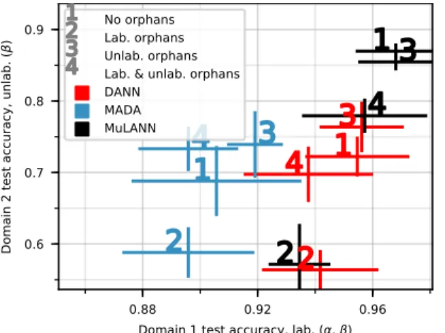
Table 3: Class content per case in the asymmetry experiments

Figure 3: Impact of asymmetry in class content between do-mains on OFFICE(W→A) for DANN, MADA and MULANN. See text for details. Better seen in color.

datapoints (Fig. 4 in Appendix). Fig. 1, right, displays the error depending onpfor various values ofp?. As could have been expected, it is better to underestimate than to overestimatep?; it is even better to slightly underestimate it than to get it right, as the entropy ranking of unlabeled examples can be perturbed by classifier errors.

Impact of class/domain asymmetry. Section 4.2 reports on the classification accuracy when all classes are represented in all domains of a given shift. In the general case however, the classes represented by the unlabeled examples are unknown, hence there might exist "orphan" classes, with labeled or unlabeled samples, unique to a single domain. The impact of such orphan classes, referred to as class asymmetry, is investigated in the 2-domain case. Four types of samples are considered (Table 3): A class might have labeled examples in both domains (α), labeled in one domain and unlabeled in the other domain (β), labeled in one domain and absent in the other one (orphanγ), and finally unlabeled in one domain and absent in the other one (orphanδ). The impact of the class asymmetry is displayed on Fig. 3, reporting the average classification accuracy ofα, βclasses on domain 1 on the x-axis, and classification accuracy of unlabeledβclasses on domain 2 on the y-axis, for MULANN, DANNand MADAon OFFICE(on CELLin Fig. 5, Appendix).

A clear trend is that adding labeled orphansγ(case "2", Fig. 3) entails a loss of accuracy for all algorithms compared to the no-orphan reference (case "1"). This is explained as follows: on the one hand, theγsamples are subject to the classifier pressure as all labeled samples; on the other hand, they must be shuffled with samples from domain 2 due to the domain discriminator(s) pressure. Thus, the easiest solution is to shuffle the unlabeledβsamples around, and the loss of accuracy on theseβ

samples is very significant (the "2" is lower on they-axis compared to "1" for all algorithms). The perturbation is less severe for the labeled(α, β)samples in domain 1, which are preserved by the classifier pressure (x-axis).

The results in case "3" are consistent with the above explanation: since the unlabeledδsamples are only seen by the discriminator(s), their addition has little impact on either the labeled or unlabeled data classification accuracy (Figs. 3 and 5). Finally, there is no clear trend in the impact of both labeled and unlabeled orphans (case "4"): labeled(α, β)(resp. unlabeledβ) are only affected for MADAon CELL(resp. MULANNon OFFICE). Overall, these results show that class asymmetry matters for practical applications of transfer learning, and can adversely affect all three adversarial methods (Figs. 3 and 5), with asymmetry in labeled class content ("2") being the most detrimental to model performance.

5

D

This paper extends the use of domain adversarial learning to multi-domain learning, establishing how theH-divergence can be used to bound both the risk across all domains and the worst-domain risk (imbalance on a specific domain). The stress is put on the notion of class asymmetry, that is, when some domains contain labeled or unlabeled examples of classes not present in other domains. Showing the significant impact of class asymmetry on the state of the art, this paper also introduces MULANN, where a new loss is meant to resist the contractive effects of the adversarial domain discriminator and to repulse (a fraction of) unlabeled examples from labeled ones in each domain.

Published as a conference paper at ICLR 2019

The merits of the approach are satisfactorily demonstrated by comparison to DANNand MADAon DIGITS, RoadSigns and OFFICE, and results obtained on the real-world CELLproblem establish a new baseline for the microscopy image community.

A perspective for further study is to bridge the gap between the proposed loss and importance sampling techniques, iteratively exploiting the latent representation to identify orphan samples and adapt the loss while learning. Further work will also focus on how to identify and preserve relevant domain-specific behaviours while learning in a domain adversarial setting (e.g., if different cell types have distinct responses to the same class of perturbations).

ACKNOWLEDGMENTS

This work was supported by NIH RO1 CA184984 (LFW), R01GM112690 (SJA) and the Institute of Computational Health Sciences at UCSF (SJA and LFW). We thank the Shoichet lab (UCSF) for access to their GPUs and Theresa Gebert for suggestions and feedback.

R

D. Michael Ando, Cory McLean, and Marc Berndl. Improving phenotypic measurements in high-content imaging screens.bioRxiv, 2017. doi: 10.1101/161422. URLhttps://www.biorxiv.org/content/ early/2017/07/10/161422.

Asha Anoosheh, Eirikur Agustsson, Radu Timofte, and Luc Van Gool. Combogan: Unrestrained scalability for image domain translation.CoRR, abs/1712.06909, 2017.

Tugkan Batu, Lance Fortnow, Ronitt Rubinfeld, Warren D. Smith, and Patrick White. Testing that distributions are close. In41st Annual Symposium on Foundations of Computer Science, FOCS 2000, 12-14 November 2000, Redondo Beach, California, USA, pp. 259–269, 2000. doi: 10.1109/SFCS.2000.892113. URL

https://doi.org/10.1109/SFCS.2000.892113.

C. Becker, C. M. Christoudias, and P. Fua. Domain adaptation for microscopy imaging. IEEE Trans Med Imaging, 34(5):1125–1139, May 2015.

Shai Ben-David, John Blitzer, Koby Crammer, and Fernando Pereira. Analysis of representations for domain adaptation. InProceedings of the 19th International Conference on Neural Information Processing

Sys-tems, NIPS’06, pp. 137–144, Cambridge, MA, USA, 2006. MIT Press. URLhttp://dl.acm.org/

citation.cfm?id=2976456.2976474.

Shai Ben-David, John Blitzer, Koby Crammer, Alex Kulesza, Fernando Pereira, and Jennifer Wortman Vaughan. A theory of learning from different domains.Machine Learning, 79(1):151–175, May 2010.

Róger Bermúdez-Chacón, Carlos Becker, Mathieu Salzmann, and Pascal Fua. Scalable unsupervised domain adaptation for electron microscopy. In Sebastien Ourselin, Leo Joskowicz, Mert R. Sabuncu, Gozde Unal, and William Wells (eds.),Medical Image Computing and Computer-Assisted Intervention – MICCAI 2016, pp. 326–334, Cham, 2016. Springer International Publishing. ISBN 978-3-319-46723-8.

Steffen Bickel, Michael Brückner, and Tobias Scheffer. Discriminative learning for differing training and test distributions. InProceedings of the 24th International Conference on Machine Learning, ICML ’07, pp. 81–88, New York, NY, USA, 2007. ACM. ISBN 978-1-59593-793-3. doi: 10.1145/1273496.1273507. URL

http://doi.acm.org/10.1145/1273496.1273507.

A. Birmingham, L. M. Selfors, T. Forster, D. Wrobel, C. J. Kennedy, E. Shanks, J. Santoyo-Lopez, D. J. Dunican, A. Long, D. Kelleher, Q. Smith, R. L. Beijersbergen, P. Ghazal, and C. E. Shamu. Statistical methods for analysis of high-throughput RNA interference screens.Nat. Methods, 6(8):569–575, Aug 2009.

K. M. Borgwardt, A. Gretton, M. J. Rasch, H. P. Kriegel, B. Scholkopf, and A. J. Smola. Integrating structured biological data by Kernel Maximum Mean Discrepancy.Bioinformatics, 22(14):49–57, Jul 2006.

Konstantinos Bousmalis, George Trigeorgis, Nathan Silberman, Dilip Krishnan, and Dumitru Erhan. Domain separation networks.CoRR, abs/1608.06019, 2016. URLhttp://arxiv.org/abs/1608.06019. Olivier Bousquet and André Elisseeff. Stability and generalization.Journal of Machine Learning Research, 2:

499–526, 2002.

P. D. Caie, R. E. Walls, A. Ingleston-Orme, S. Daya, T. Houslay, R. Eagle, M. E. Roberts, and N. O. Carragher. High-content phenotypic profiling of drug response signatures across distinct cancer cells.Mol. Cancer Ther., 9(6):1913–1926, Jun 2010.

Zhangjie Cao, Mingsheng Long, Jianmin Wang, and Michael I. Jordan. Partial transfer learning with selective adversarial networks. InThe IEEE Conference on Computer Vision and Pattern Recognition (CVPR), June 2018.

Alexander Chigorin, Gleb Krivovyaz, Alexander Velizhev, and Anton Konushin. A method for traffic sign detection in an image with learning from synthetic data. In14th International Conference Digital Signal

Processing and its Applications, volume 2, pp. 316–319, 2012. URLhttp://graphics.cs.msu.ru/

files/papers/dspa2012_chigorin_ts_recognition.pdf.

Yunjey Choi, Minje Choi, Munyoung Kim, Jung-Woo Ha, Sunghun Kim, and Jaegul Choo. Stargan: Unified generative adversarial networks for multi-domain image-to-image translation. InThe IEEE Conference on Computer Vision and Pattern Recognition (CVPR), June 2018.

R. Collobert, K. Kavukcuoglu, and C. Farabet. Torch7: A matlab-like environment for machine learning. In BigLearn, NIPS Workshop, 2011.

N. Courty, R. Flamary, D. Tuia, and A. Rakotomamonjy. Optimal transport for domain adaptation. IEEE Transactions on Pattern Analysis and Machine Intelligence, 39(9):1853–1865, Sept 2017. ISSN 0162-8828. doi: 10.1109/TPAMI.2016.2615921.

Bharath Bhushan Damodaran, Benjamin Kellenberger, Rémi Flamary, Devis Tuia, and Nicolas Courty. Deepjdot: Deep joint distribution optimal transport for unsupervised domain adaptation.CoRR, abs/1803.10081, 2018. URLhttp://arxiv.org/abs/1803.10081.

Hal Daumé III and Daniel Marcu. Domain adaptation for statistical classifiers.J. Artif. Intell. Res., 26:101–126, 2006.

Mark Dredze, Alex Kulesza, and Koby Crammer. Multi-domain learning by confidence-weighted parameter com-bination.Machine Learning, 79(1):123–149, May 2010. ISSN 1573-0565. doi: 10.1007/s10994-009-5148-0. URLhttps://doi.org/10.1007/s10994-009-5148-0.

Basura Fernando, Tatiana Tommasi, and Tinne Tuytelaars. Joint cross-domain classification and subspace learning for unsupervised adaptation. Pattern Recognition Letters, 65:60–66, 2015. doi: 10.1016/j.patrec. 2015.07.009. URLhttps://doi.org/10.1016/j.patrec.2015.07.009.

Yaroslav Ganin, Evgeniya Ustinova, Hana Ajakan, Pascal Germain, Hugo Larochelle, François Laviolette, Mario Marchand, and Victor Lempitsky. Domain-adversarial training of neural networks. Journal of Machine

Learning Research, 17(59):1–35, 2016. URLhttp://jmlr.org/papers/v17/15-239.html.

Muhammad Ghifary, W. Bastiaan Kleijn, Mengjie Zhang, David Balduzzi, and Wen Li. Deep reconstruction-classification networks for unsupervised domain adaptation. InComputer Vision - ECCV, pp. 597–613, 2016.

Boqing Gong, Kristen Grauman, and Fei Sha. Connecting the dots with landmarks: Discriminatively learning domain-invariant features for unsupervised domain adaptation. InProceedings of the 30th International Conference on International Conference on Machine Learning - Volume 28, ICML’13, pp. I–222–I–230. JMLR.org, 2013. URLhttp://dl.acm.org/citation.cfm?id=3042817.3042844.

Arthur Gretton, Karsten M. Borgwardt, Malte J. Rasch, Bernhard Schölkopf, and Alexander J. Smola. A kernel method for the two-sample-problem. InNIPS, pp. 513–520. MIT Press, 2007.

Jiayuan Huang, Alexander J. Smola, Arthur Gretton, Karsten M. Borgwardt, and Bernhard Scholkopf. Correcting sample selection bias by unlabeled data. InProceedings of the 19th International Conference on Neural Information Processing Systems, NIPS’06, pp. 601–608, Cambridge, MA, USA, 2006. MIT Press. URL

http://dl.acm.org/citation.cfm?id=2976456.2976532.

Phillip Isola, Jun-Yan Zhu, Tinghui Zhou, and Alexei A. Efros. Image-to-image translation with conditional adversarial networks. InCVPR, pp. 5967–5976. IEEE Computer Society, 2017.

Yangqing Jia, Evan Shelhamer, Jeff Donahue, Sergey Karayev, Jonathan Long, Ross Girshick, Sergio Guadar-rama, and Trevor Darrell. Caffe: Convolutional architecture for fast feature embedding. arXiv preprint arXiv:1408.5093, 2014.

Eric Jones, Travis Oliphant, Pearu Peterson, et al. SciPy: Open source scientific tools for Python, 2001–. URL

Published as a conference paper at ICLR 2019

Konstantinos Kamnitsas, Christian Baumgartner, Christian Ledig, Virginia Newcombe, Joanna Simpson, Andrew Kane, David Menon, Aditya Nori, Antonio Criminisi, Daniel Rueckert, and Ben Glocker. Unsupervised domain adaptation in brain lesion segmentation with adversarial networks. In Marc Niethammer, Martin Styner, Stephen Aylward, Hongtu Zhu, Ipek Oguz, Pew-Thian Yap, and Dinggang Shen (eds.),Information Processing in Medical Imaging, pp. 597–609, Cham, 2017. Springer International Publishing. ISBN 978-3-319-59050-9.

J. Kang, C. H. Hsu, Q. Wu, S. Liu, A. D. Coster, B. A. Posner, S. J. Altschuler, and L. F. Wu. Improving drug discovery with high-content phenotypic screens by systematic selection of reporter cell lines.Nat. Biotechnol., 34(1):70–77, Jan 2016.

Daniel Kifer, Shai Ben-David, and Johannes Gehrke. Detecting change in data streams. InProceedings of the Thirtieth International Conference on Very Large Data Bases - Volume 30, VLDB ’04, pp. 180–191. VLDB Endowment, 2004. ISBN 0-12-088469-0. URLhttp://dl.acm.org/citation.cfm?id= 1316689.1316707.

Piotr Koniusz, Yusuf Tas, and Fatih Porikli. Domain adaptation by mixture of alignments of second- or higher-order scatter tensors.CoRR, abs/1611.08195, 2016. URLhttp://arxiv.org/abs/1611.08195. Alex Krizhevsky, Ilya Sutskever, and Geoffrey E Hinton. Imagenet classification with

deep convolutional neural networks. In F. Pereira, C. J. C. Burges, L. Bottou, and K. Q. Weinberger (eds.), Advances in Neural Information Processing Systems 25, pp. 1097–1105. Curran Associates, Inc., 2012. URL http://papers.nips.cc/paper/ 4824-imagenet-classification-with-deep-convolutional-neural-networks. pdf.

Y. Le Cun, L. Bottou, Y. Bengio, and P. Haffner. Gradient-based learning applied to document recognition. Proceedings of the IEEE, 86(11):2278–2324, Nov 1998. ISSN 0018-9219. doi: 10.1109/5.726791. Ming-Yu Liu, Thomas Breuel, and Jan Kautz. Unsupervised image-to-image translation

net-works. In I. Guyon, U. V. Luxburg, S. Bengio, H. Wallach, R. Fergus, S. Vish-wanathan, and R. Garnett (eds.), Advances in Neural Information Processing Systems 30, pp. 700–708. Curran Associates, Inc., 2017. URL http://papers.nips.cc/paper/ 6672-unsupervised-image-to-image-translation-networks.pdf.

V. Ljosa, K. L. Sokolnicki, and A. E. Carpenter. Annotated high-throughput microscopy image sets for validation. Nat. Methods, 9(7):637, Jun 2012.

Mingsheng Long, Yue Cao, Jianmin Wang, and Michael I. Jordan. Learning transferable features with deep adaptation networks. InProceedings of the 32Nd International Conference on International Conference on

Machine Learning - Volume 37, ICML’15, pp. 97–105. JMLR.org, 2015. URLhttp://dl.acm.org/

citation.cfm?id=3045118.3045130.

Mingsheng Long, Jianmin Wang, and Michael I. Jordan. Deep transfer learning with joint adaptation networks.

CoRR, abs/1605.06636, 2016. URLhttp://arxiv.org/abs/1605.06636.

Mingsheng Long, Zhangjie Cao, Jianmin Wang, and Michael I. Jordan. Domain adaptation with randomized multilinear adversarial networks.CoRR, abs/1705.10667, 2017. URLhttp://arxiv.org/abs/1705. 10667.

Yishay Mansour. Learning and domain adaptation. InAlgorithmic Learning Theory, 20th International Conference, ALT, pp. 4–6, 2009.

Yishay Mansour, Mehryar Mohri, and Afshin Rostamizadeh. Domain adaptation with multiple sources. In Proceedings of the 21st International Conference on Neural Information Processing Systems, NIPS’08, pp. 1041–1048, USA, 2008. Curran Associates Inc. ISBN 978-1-6056-0-949-2. URLhttp://dl.acm.org/ citation.cfm?id=2981780.2981910.

Saeid Motiian, Marco Piccirilli, Donald A. Adjeroh, and Gianfranco Doretto. Unified deep supervised domain adaptation and generalization. InThe IEEE International Conference on Computer Vision (ICCV), Oct 2017. Krikamol Muandet, David Balduzzi, and Bernhard Schölkopf. Domain generalization via invariant feature representation. InProceedings of the 30th International Conference on International Conference on

Ma-chine Learning - Volume 28, ICML’13, pp. I–10–I–18. JMLR.org, 2013. URLhttp://dl.acm.org/

citation.cfm?id=3042817.3042820.

Nobuyuki Otsu. A Threshold Selection Method from Gray-level Histograms.IEEE Transactions on Systems,

Man and Cybernetics, 9(1):62–66, 1979. doi: 10.1109/TSMC.1979.4310076. URLhttp://dx.doi.

S. J. Pan and Q. Yang. A survey on transfer learning.IEEE Transactions on Knowledge and Data Engineering, 22(10):1345–1359, Oct 2010. ISSN 1041-4347.

Zhongyi Pei, Zhangjie Cao, Mingsheng Long, and Jianmin Wang. Multi-adversarial domain adaptation. In

Proceedings of the 32nd AAAI Conference on Artificial Intelligence, 2018. URLhttps://www.aaai.

org/ocs/index.php/AAAI/AAAI18/paper/view/17067.

L. Y. Pratt, J. Mostow, and C. A. Kamm. Direct transfer of learned information among neural networks. In Proceedings of the Ninth National Conference on Artificial Intelligence (AAAI-91), AAAI’91, pp. 584–589. Anaheim, CA, 1991. URLhttps://www.aaai.org/Papers/AAAI/1991/AAAI91-091.pdf. S. Preibisch, S. Saalfeld, and P. Tomancak. Globally optimal stitching of tiled 3D microscopic image acquisitions.

Bioinformatics, 25(11):1463–1465, Jun 2009.

Olga Russakovsky, Jia Deng, Hao Su, Jonathan Krause, Sanjeev Satheesh, Sean Ma, Zhiheng Huang, Andrej Karpathy, Aditya Khosla, Michael Bernstein, Alexander C. Berg, and Li Fei-Fei. ImageNet Large Scale Visual Recognition Challenge. International Journal of Computer Vision (IJCV), 115(3):211–252, 2015. doi: 10.1007/s11263-015-0816-y.

Kate Saenko, Brian Kulis, Mario Fritz, and Trevor Darrell. Adapting visual category models to new domains. In Kostas Daniilidis, Petros Maragos, and Nikos Paragios (eds.),Computer Vision – ECCV 2010, pp. 213–226, Berlin, Heidelberg, 2010. Springer Berlin Heidelberg. ISBN 978-3-642-15561-1.

Swami Sankaranarayanan, Yogesh Balaji, Carlos D. Castillo, and Rama Chellappa. Generate to adapt: Aligning domains using generative adversarial networks.CoRR, abs/1704.01705, 2017. URLhttp://arxiv.org/ abs/1704.01705.

C. A. Schneider, W. S. Rasband, and K. W. Eliceiri. NIH Image to ImageJ: 25 years of image analysis.Nat. Methods, 9(7):671–675, Jul 2012.

Gabriele Schweikert, Christian Widmer, Bernhard Schölkopf, and Gunnar Rätsch. An empirical analysis of domain adaptation algorithms for genomic sequence analysis. InProceedings of the 21st International Confer-ence on Neural Information Processing Systems, NIPS’08, pp. 1433–1440, USA, 2008. Curran Associates Inc. ISBN 978-1-6056-0-949-2. URLhttp://dl.acm.org/citation.cfm?id=2981780.2981959. Hidetoshi Shimodaira. Improving predictive inference under covariate shift by weighting the log-likelihood

function.Journal of Statistical Planning and Inference, 90(2):227–244, 2000.

Rui Shu, Hung H. Bui, Hirokazu Narui, and Stefano Ermon. A DIRT-T approach to unsupervised domain adaptation. InProceedings of the 6th International Conference on Learning Representations (ICLR), 2018. A. Sigal, R. Milo, A. Cohen, N. Geva-Zatorsky, Y. Klein, I. Alaluf, N. Swerdlin, N. Perzov, T. Danon, Y. Liron,

T. Raveh, A. E. Carpenter, G. Lahav, and U. Alon. Dynamic proteomics in individual human cells uncovers widespread cell-cycle dependence of nuclear proteins.Nat. Methods, 3(7):525–531, Jul 2006.

Karen Simonyan and Andrew Zisserman. Very deep convolutional networks for large-scale image recognition.

CoRR, abs/1409.1556, 2014. URLhttp://arxiv.org/abs/1409.1556.

J. Stallkamp, M. Schlipsing, J. Salmen, and C. Igel. Man vs. computer: Benchmarking machine learn-ing algorithms for traffic sign recognition. Neural Networks, pp. –, 2012. ISSN 0893-6080. doi: 10.1016/j.neunet.2012.02.016. URL http://www.sciencedirect.com/science/article/ pii/S0893608012000457.

T. Stoeger, N. Battich, M. D. Herrmann, Y. Yakimovich, and L. Pelkmans. Computer vision for image-based transcriptomics.Methods, 85:44–53, Sep 2015.

Baochen Sun and Kate Saenko. Deep coral: Correlation alignment for deep domain adaptation. In Gang Hua and Hervé Jégou (eds.),Computer Vision – ECCV 2016 Workshops, pp. 443–450, Cham, 2016. Springer International Publishing. ISBN 978-3-319-49409-8.

Baochen Sun, Jiashi Feng, and Kate Saenko. Return of frustratingly easy domain adaptation. InProceedings

of the 29th AAAI Conference on Artificial Intelligence, AAAI, 2016. URLhttp://arxiv.org/abs/

1511.05547.

Yaniv Taigman, Adam Polyak, and Lior Wolf. Unsupervised cross-domain image generation. CoRR, abs/1611.02200, 2016. URLhttp://arxiv.org/abs/1611.02200.

E. Tzeng, J. Hoffman, T. Darrell, and K. Saenko. Simultaneous deep transfer across domains and tasks.

In 2015 IEEE International Conference on Computer Vision (ICCV), pp. 4068–4076, Dec 2015. doi:

Published as a conference paper at ICLR 2019

Eric Tzeng, Judy Hoffman, Ning Zhang, Kate Saenko, and Trevor Darrell. Deep domain confusion: Maximizing for domain invariance.CoRR, abs/1412.3474, 2014. URLhttp://arxiv.org/abs/1412.3474. Eric Tzeng, Judy Hoffman, Kate Saenko, and Trevor Darrell. Adversarial discriminative domain adaptation.

CoRR, abs/1702.05464, 2017. URLhttp://arxiv.org/abs/1702.05464.

Francesco Vallania, Andrew Tam, Shane Lofgren, Steven Schaffert, Tej D. Azad, Erika Bongen, Meia Alsup, Michael Alonso, Mark Davis, Edgar Engleman, and Purvesh Khatri. Leveraging heterogeneity across multiple data sets increases accuracy of cell-mixture deconvolution and reduces biological and technical biases.bioRxiv, 2017. doi: 10.1101/206466. URLhttps://www.biorxiv.org/content/early/2017/10/20/ 206466.

Laurens van der Maaten and Geoffrey Hinton. Visualizing data using t-SNE. Journal of Machine Learning

Research, 9:2579–2605, 2008. URLhttp://www.jmlr.org/papers/v9/vandermaaten08a.

html.

Annegreet van Opbroek, M. Arfan Ikram, Meike W. Vernooij, and Marleen de Bruijne. Transfer learning improves supervised image segmentation across imaging protocols.I E E E Transactions on Medical Imaging, 34(5):1018–1030, 2015. ISSN 0278-0062. doi: 10.1109/TMI.2014.2366792.

V. N. Vapnik.Statistical Learning Theory. Wiley, 1998.

Tong Xiao, Hongsheng Li, Wanli Ouyang, and Xiaogang Wang. Learning deep feature representations with domain guided dropout for person re-identification. InProceedings of the **th Conference on Computer

Vision and Pattern Recognition, CVPR’16, 2016. URLhttp://arxiv.org/abs/1604.07528.

Qian Xu and Qiang Yang. A Survey of Transfer and Multitask Learning in Bioinformatics.Journal of Computing Science and Engineering, August 2011.

Yongxin Yang and Timothy M. Hospedales. A unified perspective on multi-domain and multi-task learning. In Proceedings of the 3d International Conference on Representation Learning, ICLR’15, 2015.

Zili Yi, Hao (Richard) Zhang, Ping Tan, and Minglun Gong. Dualgan: Unsupervised dual learning for image-to-image translation. InICCV, pp. 2868–2876. IEEE Computer Society, 2017.

Chao Zhang, Lei Zhang, and Jieping Ye. Generalization bounds for domain adaptation. In F. Pereira, C. J. C. Burges, L. Bottou, and K. Q. Weinberger (eds.),Advances in Neural Information Processing

Systems 25, pp. 3320–3328. Curran Associates, Inc., 2012. URLhttp://papers.nips.cc/paper/

4684-generalization-bounds-for-domain-adaptation.pdf.

Jing Zhang, Zewei Ding, Wanqing Li, and Philip Ogunbona. Importance weighted adversarial nets for partial domain adaptation.CoRR, abs/1803.09210, 2018. URLhttp://arxiv.org/abs/1803.09210. Jun-Yan Zhu, Taesung Park, Phillip Isola, and Alexei A. Efros. Unpaired image-to-image translation using

A

E

-

-

-

:

In the field of computer vision, another way of mapping examples in one domain onto the other domain is image-to-image translation. In the supervised case (the true pairs made of an image and its translation are given), Pic2Pix (Isola et al., 2017) trains a conditional GAN to discriminate true pairs from fake ones. In the unsupervised case, another loss is designed to enforce cycle consistency (simultaneously learning the mappingφfrom domainAtoB,ψfromBtoA, and requiringφoψ=Id) (Zhu et al., 2017; Yi et al., 2017). Note that translation approaches do notper seaddress domain adaptation as they are agnostic w.r.t. the classes. Additional losses are used to overcome this limitation: Domain transfer network (DTN) (Taigman et al., 2016) uses an auto-encoder-like loss in the latent space; GenToAdapt (Sankaranarayanan et al., 2017) uses a classifier loss in the latent space; UNIT (Liu et al., 2017) uses a VAE loss.

StarGAN (Choi et al., 2018) combines image-to-image translation with a GAN, where the discrimina-tor is trained to discriminate true from fake pairs on the one hand, and the domain on the other hand. ComboGAN (Anoosheh et al., 2017) learns two networks per domain, an encoder and a decoder. DIRT-T (Shu et al., 2018) uses a conditional GAN and a classifier in the latent space, with two additional losses, respectively enforcing the cluster assumption (the classifier boundary should not cross high density region) and a virtual adversarial training (the hypothesis should be invariant under slight perturbations of the input).

Interestingly, DA and MDL (like deep learning in general) tend to combine quite some losses; two benefits are expected from using a mixture of losses, a smoother optimization landscape and a good stability of the representation (Bousquet & Elisseeff, 2002).

B

P

B.1 DEFINITION OF THEH-DIVERGENCE

Definition. (Kifer et al., 2004; Ben-David et al., 2006; 2010) Given a domainX, two distributions DandD0_{over that domain and a binary hypothesis classHonX, theH-divergence betweenDand}

D0_{is defined as:}

dH(D,D0) = 2 sup

h∈H

|_PD(h(x) = 1)−PD0(h(x) = 1)|

B.2 BOUNDINGMDLLOSS USING THEH-DIVERGENCE

Theorem 2. Given an input spaceX, we considerndistributionsDioverX ×{0; 1}and a hypothesis classHonX of VC dimensiond. Letαandγbe in the simplex of dimensionn. IfSis a sample of sizemwhich containsγimsamples fromDi, andhˆis the empirical minimizer ofP_iαiˆion(Si)i, then for anyδ >0, with probability at least1−δ, the compound empirical error is upper bounded as: X i i(ˆh)≤ X i ?_i + 4nB(α) + 2X i≤j (αi+αj) dH(DXi ,D X j ) +βi,j (5) with B(α) = v u u t X j α2_j γj s 2dlog(2(m+ 1)) + log(4_δ) m and βi,j=min h∈H (i(h) +j(h))

A tighter bound can be obtained by replacing dH(Di,Dj) with 12dH∆H(Di,Dj). The H∆H

-divergence (Ben-David et al., 2010) operates on the symmetric difference hypothesis spaceH∆H. However, divergenceH∆Hdoes not lend itself to empirical estimation: even Ben-David et al. (2010) fall back onH-divergence in their empirical validation.

Published as a conference paper at ICLR 2019

Proof of theorem 2 Fori, jwe noteβi,j =i(h?i,j) +j(h?i,j) =min

h∈H(i(h) +j(h)). Forαin

then-dimensional simplex andh∈ H, we noteα(h) =P_iαii(h).

We have forαin the simplex of dimensionn,h∈ Handj ∈ {1, . . . , m}, using the triangle inequality (similarly to the proof of Theorem 4 in (Ben-David et al., 2010))

|α(h)−j(h)|= X i αi Ex,y∼Di|h(x)−y| −Ex,y∼Dj|h(x)−y| ≤X i αi Ex,y∼Di|h(x)−y| −Ex,y∼Dj|h(x)−y| ≤X i αi Ex,y∼Di|h(x)−y| −Ex∼Di|h(x)−h ? i,j(x)| +αi _Ex∼Di|h(x)−h ? i,j(x)| −Ex∼Dj|h(x)−h ? i,j(x)| +αi Ex∼Dj|h(x)−h ? i,j(x)| −Ex,y∼Dj|h(x)−y| ≤X i αi(βi,j+dH(Di,Dj))

The last line follows from the definitions ofβi,jandH-divergence. Thus using lemma 6 in (Ben-David et al., 2010) j(ˆh)≤α(ˆh) + X i αi(βi,j+dH(Di,Dj)) ≤ˆα(ˆh) + 2B(α) + X i αi(βi,j+dH(Di,Dj)) ≤ˆα(h?j) + 2B(α) + X i αi(βi,j+dH(Di,Dj)) ≤α(h?j) + 4B(α) + X i αi(βi,j+dH(Di,Dj)) ≤?i + 4B(α) + 2 X i αi(βi,j+dH(Di,Dj)) with B(α) = v u u t X j α2_j βj s 2dlog(2(m+ 1)) + log(4 δ) m

Hence the result.

B.3 BOUNDING DOMAIN IMBALANCE

Proof of proposition 1 We have forh∈ Handj∈[1, . . . , m], using the triangle inequality and the definition of?

i (similarly to the proof of Theorem 1 in (Ben-David et al., 2006))

j(h) =Px,y∼Dj(h(x)6=y) =_Ex,y∼Dj|h(x)−y| ≤EDX j |h(x)−h ? j(x)|+EDj|h ? j(x)−y| ≤EDX j |h(x)− 1 n X i h?_i(x)|+EDX j | 1 n X i h?_i(x)−h_j?(x)|+?_j ≤ 1 n X i EDX j |h(x)−h ? i(x)|+ 1 n X i EDX j |h ? i(x)−h ? j(x)|+ ? j

We have fori EDX j |h(x)−h ? i(x)| ≤EDX i |h(x)−h ? i(x)|+|EDX i |h(x)−h ? i(x)| −EDX j |h(x)−h ? i(x)|| ≤i(h) +?i +dH(DiX,DjX)

The second line follows from the triangle inequality and the definition of theH-divergence. Thus

j(h)≤ 1 n X i i(h) +?i +dH(DiX,D X j ) +EDX j |h ? i(x)−h ? j(x)| +?_j (6) By symmetry we obtain 1 n X i i(h)≤j(h) + 1 n X i ?_i +dH(DXi ,D X j ) +EDX i |h ? i(x)−h ? j(x)| +?_j

Thus the result.

Proposition 3. Given a domainX,mdistributionsDioverX × {0; 1}and a hypothesis classHon X, we have forh∈ Handj∈[1, . . . , m]

|j(h)− 1 n X i i(h)| ≤2 ?j+ 1 n X i ?_i ! +j(h?) +β+ 1 n X i dH(DXi ,D X j ) + 1 2dH∆H(Di,Dj) (7) where β =X j j(h?) =min h∈H X j j(h)

Proof Fori, j∈[i, . . . , m]we have EDi|h ? i(x)−h ? j(x)| ≤EDi|h ? j(x)−h ?_(x)|+ EDi|h ?_(x)−h? i(x)| ≤EDj|h ? j(x)−h?(x)|+12dH∆H(Di,Dj) +i(h ?_{) +}? i ≤i(h?) +j(h?) +?i + ? j+ 1 2dH∆H(Di,Dj)

The second line follows from Lemma 3 from (Ben-David et al., 2010), and the third from the triangle inequality. From this and proposition 1 we obtain the result.

Corollaries for the 2-domain case

Corollary 4. Given a domainX, two distributionsDSandDT overX × {0,1}and a hypothesis classHonX, we have forh∈ H

|S(h)−T(h)| ≤?T + ? S+ ∆ +dH(DXS,D X T) (8) with∆ =max(E_DX T|h ? S(x)−h?T(x)|, EDX S|h ? S(x)−h?T(x)|)

Corollary 5. Given a domainX, two distributionsDSandDT overX × {0; 1}and a hypothesis classHonX, we have forh∈ H

|S(h)−T(h)| ≤2(?T + ? S) +β+ 1 2dH∆H(DS,DT) +dH(D X S,D X T) (9) where β =S(h?) +T(h?) =min h∈HS(h) +T(h)

C

C

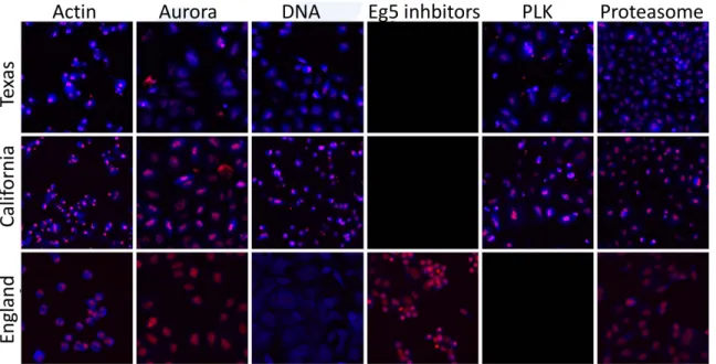
This dataset is extracted from that published in (Kang et al., 2016). It contains 455 biologically active images, in 11 classes, on four 384-well plates, in three channels: H2B-CFP, XRCC5-YFP and cytoplasmic-mCherry. Our analysis used 10 classes: ’Actin’, ’Aurora’, ’DNA’, ’ER’, ’HDAC’, ’Hsp90’, ’MT’, ’PLK’, ’Proteasome’, ’mTOR’.

On top of the quality control from the original paper, a visual quality control was implemented to remove images with only apoptotic cells, and XRCC5-YFP channel images were smoothed using a median filter of size 2 using SciPy (Jones et al., 2001–).

Published as a conference paper at ICLR 2019

Figure 2: Examples from six classes in the Bio dataset (red: cell nuclei, blue: cell cytoplasm, magnification: 10X). Empty squares: the domain does not contain any known examples from this class. Best seen in color.

C.2 CALIFORNIA DOMAIN

This dataset is designed to be similar to the Texas domain (Kang et al., 2016), generated using the same cell line, but in a different laboratory, by a different biologist, and using different equipment. It contains 1,077 biologically active images, in 10 classes, on ten 384-well plates, in three channels: H2B-CFP, XRCC5-YFP and cytoplasmic-mCherry. The classes are: ’Actin’, ’Aurora’, ’DNA’, ’ER’, ’HDAC’, ’Hsp90’, ’MT’, ’PLK’, ’Proteasome’, ’mTOR’.

Cell culture, drug screening and image acquisition Previously (Kang et al., 2016), retroviral transduction of a marker plasmid "pSeg" was used to stably express H2B-CFP and cytoplasmic-mCherry tags in A549 human lung adenocarcinoma cells. A CD-tagging approach (Sigal et al., 2006) was used to add an N-terminal YFP tag to endogenous XRCC5.

Cells were maintained in RPMI1640 media containing 10% FBS, 2 mM glutamine, 50 units/ml penicillin, and 50µg/ml streptomycin (all from Life Technologies, Inc.), at37◦C, 5% CO2_and

100% humidity. 24h prior to drug addition, cells were seeded onto 384-well plate at a density of 1200 cells/well. Following compound addition, cells were incubated at37◦Cfor 48 hours. Images were then acquired using a GE InCell Analyzer 2000. One image was acquired per well using a 10x objective lens with 2x2 binning.

Image processing Uneven illumination was corrected as described in (Stoeger et al., 2015). Back-ground noise was removed using the ImageJ RollingBall plugin (Schneider et al., 2012). Images were segmented, object features extracted and biological activity determined as previously described (Kang et al., 2016). A visual quality control was implemented to remove images with obvious anomalies (e.g. presence of a hair or out-of-focus image) and images with only apoptotic cells. YFP-XRCC5 channel images were smoothed using a median filter of size 2.

C.3 ENGLAND DOMAIN

This dataset was published by Caie et al. (2010) and retrieved from (Ljosa et al., 2012). It contains 879 biologically active images of MCF7 breast adenocarcinoma cells, in 15 classes on 55 96-well plates, in 3 channels: Alexa Fluor 488 (Tubulin), Alexa Fluor 568 (Actin) and DAPI (nuclei). Classes with fewer than 15 images and absent from the other datasets ("Calcium regulation", "Cholesterol",

"Epithelial", "MEK", "mTOR") were not used, which leaves 10 classes: ’Actin’, ’Aurora’, ’DNA’, ’ER’, ’Eg5 inhibitor’, ’HDAC’, ’Kinase’, ’MT’, ’Proteasome’, ’Protein synthesis’.

Image processing As the images were acquired using a 20X objective, they were stitched using ImageJ plugin (Preibisch et al., 2009) and down-scaled 2 times. Cells thus appear the same size as in the other domains. Images were segmented, object features extracted and biological activity obtained as previously described (Kang et al., 2016). A visual quality control was implemented to remove images with obvious anomalies and images with only apoptotic cells. Images with too few cells were also removed: an Otsu filter (Otsu, 1979) was used to estimate the percentage of pixels containing nuclei in each image, and images with less than 1% nuclear pixels were removed. Tubulin channel images were smoothed using a median filter of size 2.

C.4 COMMON IMAGE PRE-PROCESSING

Images which were not significantly distinct from negative controls were identified as previ-ously (Kang et al., 2016) and excluded from our analysis. Previous work on the England dataset further focused on images which "clearly [have] one of 12 different primary mechanims of ac-tion" (Ljosa et al., 2012). We chose not to do so, since it results in a simpler problem (90% accuracy easy to reach) with much less room for improvement.

Images from all domains were down-scaled 4 times and flattened to form RGB images. Images were normalized by subtracting the intensity values from negative controls (DMSO) of the same plate in each channel. England, Texas and California share images for cell nucleus and cytoplasm, but their third channel differs: Texas and California shows the protein XRCC5, whereas England shows the Actin protein. Therefore, the experiments which combine Texas and England, and California and England used only the first two channels, feeding an empty third channel into the network. Similarly, profiles contain 443 features which are related to the first two channels, and 202 features which are related to the third channel. Only the former were used in experiments which involve the England dataset.

C.5 SEMI-SUPERVISEDMDLEXPERIMENTS

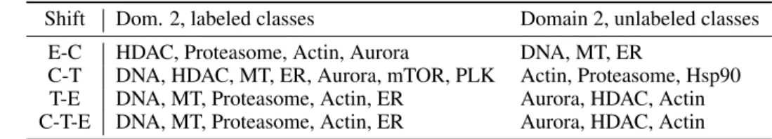
Shift Dom. 2, labeled classes Domain 2, unlabeled classes E-C HDAC, Proteasome, Actin, Aurora DNA, MT, ER

C-T DNA, HDAC, MT, ER, Aurora, mTOR, PLK Actin, Proteasome, Hsp90 T-E DNA, MT, Proteasome, Actin, ER Aurora, HDAC, Actin C-T-E DNA, MT, Proteasome, Actin, ER Aurora, HDAC, Actin

Table 3: Class content for the CELLexperiments in table 2. In all cases, the first domain contains the same classes as domain 2, though with labeled examples from all classes. These classes were picked as those with best classification accuracy in an unsupervised setting; results are similar when picking the classes with worst classification accuracy. 10 labeled images per class were used for training.

Published as a conference paper at ICLR 2019

D

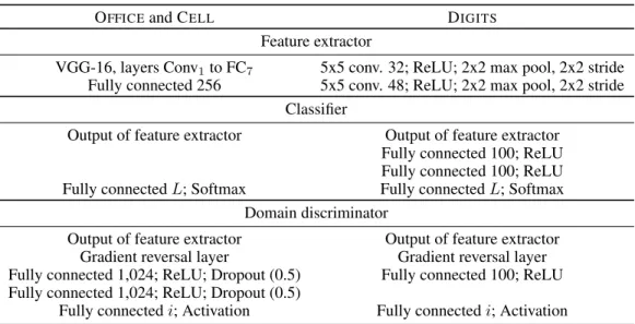
E

As in (Ganin et al., 2016; Tzeng et al., 2014), a bottleneck fully connected layer is added after the last dense layer of VGG-16. Learning rates on weights (resp. biases) from "from scratch" layers is ten (resp, twenty) times that on parameters of fine-tuned layers. Instance normalization is used on DIGITS, whereas global normalization is used on OFFICEand CELL.

OFFICEand CELL DIGITS

Feature extractor

VGG-16, layers Conv1to FC7 5x5 conv. 32; ReLU; 2x2 max pool, 2x2 stride

Fully connected 256 5x5 conv. 48; ReLU; 2x2 max pool, 2x2 stride Classifier

Output of feature extractor Output of feature extractor Fully connected 100; ReLU Fully connected 100; ReLU Fully connectedL; Softmax Fully connectedL; Softmax

Domain discriminator

Output of feature extractor Output of feature extractor Gradient reversal layer Gradient reversal layer Fully connected 1,024; ReLU; Dropout (0.5) Fully connected 100; ReLU Fully connected 1,024; ReLU; Dropout (0.5)

Fully connectedi; Activation Fully connectedi; Activation

Table 4: Architectures. In the case when considering only two domains,i= 1and the last activation of domain discriminators is a sigmoid. When considering three domains,i= 3and the activation is a softmax. Knowledge discriminator architecture is identical to that of domain discriminators without the gradient reversal layer.

D.2 HYPER-PARAMETER SEARCH

Parameter DIGITSand Signs CELL

Learning rate (lr) 10−3_,10−4 ₁₀−4₍₊₁₀−5_{for 3-dom.)}

Individual lr NA True, False

Lr schedule Exponentially decreasing, constant

λ 0.1,0.8

λschedule Exponentially increasing, constant

ζ 0.1,0.8

Table 5: Range of hyper-parameters which were evaluated in cross-validation experiments. Exponen-tially decreasing schedule, exponenExponen-tially increasing schedule, indiv. lr (learning rates from layers which were trained from scratch are multiplied by 10), as in (Ganin et al., 2016).

E

A

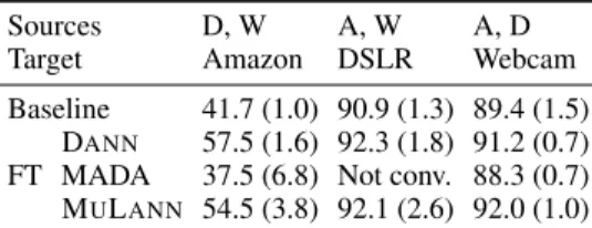
Table 6: Classification results on target test set in the semi-supervised DA setting (average and stdev on 5 seeds or folds)

Sources D, W A, W A, D

Target Amazon DSLR Webcam

Baseline 41.7 (1.0) 90.9 (1.3) 89.4 (1.5) FT

DANN 57.5 (1.6) 92.3 (1.8) 91.2 (0.7) MADA 37.5 (6.8) Not conv. 88.3 (0.7) MULANN 54.5 (3.8) 92.1 (2.6) 92.0 (1.0)

Published as a conference paper at ICLR 2019

DANN

MADA

MuLANN

Figure 3: Visualization of class features on Webcam (red) > Amazon (blue). Dimmer colors indicate classes for which labeled examples are available in both domains.

E.2 TSNEVISUALIZATION

We use tSNE (van der Maaten & Hinton, 2008) to visualize the common feature space in the example of Webcam→Amazon. Fig. 3 shows that classes are overall better separated with MULANN. In particular, when using MULANN, unlabeled examples (blue) are both more grouped and closer to labeled points from the other domain.

E.3 SEMI-SUPERVISEDMDLON THEBIO DATASET

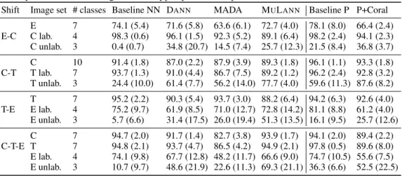
Table 5: CELLaverage test classification results on all domain (average and stdev on 5 folds). P stands for "profiles", "lab." for labeled and "unlab." for unlabeled. Baselines are obtained by training MULANNwithλ = 0(NN) and LDA+k-NN (P) on both domains. Results were obtained in the non-fully transductive setting, without hyper-parameter optimization.

Shift Image set # classes Baseline NN DANN MADA MULANN Baseline P P+Coral

E-C E 7 74.1 (5.4) 71.6 (5.8) 63.6 (6.1) 72.7 (4.0) 78.1 (8.0) 66.4 (2.4) C lab. 4 98.3 (0.6) 96.1 (1.5) 92.3 (5.2) 89.1 (6.4) 98.2 (2.4) 94.1 (2.3) C unlab. 3 0.4 (0.7) 34.8 (20.7) 14.5 (7.4) 25.7 (12.3) 21.5 (8.4) 36.8 (3.7) C-T C 10 91.4 (1.8) 87.0 (2.2) 87.9 (3.9) 89.3 (1.8) 96.1 (1.1) 93.3 (1.8) T lab. 7 93.7 (1.3) 91.0 (4.4) 86.7 (7.5) 89.2 (1.2) 96.2 (2.4) 92.8 (3.2) T unlab. 3 24.4 (10.0) 61.4 (7.7) 56.2 (14.0) 77.7 (4.0) 59.6 (11.3) 87.6 (8.2) T-E T 7 95.2 (2.2) 90.3 (5.4) 93.7 (3.0) 88.2 (6.4) 94.2 (6.3) 92.6 (4.0) E lab. 4 75.2 (9.7) 61.9 (8.5) 71.0 (12.7) 72.8 (14.2) 81.1 (8.8) 61.2 (4.0) E unlab. 3 5.7 (6.6) 31.4 (17.5) 26.0 (19.4) 51.3 (13.5) 16.1 (9.5) 25.7 (12.6) C-T-E C 7 94.7 (2.0) 91.7 (1.4) 82.7 (3.8) 93.9 (1.7) 94.1 (2.0) 89.4 (2.2) T 7 94.8 (2.1) 93.7 (4.7) 86.5 (4.2) 94.9 (2.1) 97.8 (0.5) 89.6 (8.0) E lab. 4 74.1 (9.8) 67.7 (12.8) 48.2 (11.7) 66.6 (9.0) 74.7 (10.5) 55.6 (7.5) E unlab. 3 10.7 (9.7) 48.6 (21.9) 22.6 (11.3) 69.3 (21.1) 36.3 (6.6) 52.5 (22.5)

E.4 IMPACT OFp−p?ON A DOMAIN WITHOUT UNLABELED DATAPOINTS E.5 ASYMMETRY RESULTS ONCELL

Published as a conference paper at ICLR 2019 0.0 0.3 0.5 0.7 1.0 p 0.00 0.05 0.10 0.15 0.20 0.25

Test error on MNIST

p =0.3 p =0.5 p =0.7 p =1 Labeled data Unlabeled data

Figure 4: Impact of parameterpin comparison withp?_{on MNIST↔MNIST-M.p= 0corresponds} to DANN (see text for details): no data flowed through the KUD module. We can see that different values of(p, p?_{)do not influence the accuracy on a domain which did not have any unlabaled} datapoints from extra classes (MNIST in this case).

0.72 0.76 0.80 0.84 0.88 0.92 0.96 Domain 1 test accuracy, lab. ( , )

0.2 0.3 0.4 0.5 0.6 0.7 0.8 Do m ain 2 te st ac cu ra cy , u nla b. ( ) No orphans Lab. orphans Unlab. orphans Lab. & unlab. orphans DANN

MADA MuLANN

Figure 5: Impact of asymmetry in class content between domains on CELL(T↔E) for DANN, MADA and MULANN.