City, University of London Institutional Repository
Citation:
Bischofberger, S., Hiabu, M., Mammen, E. and Nielsen, J. P. ORCID:
0000-0002-2798-0817 (2019). A comparison of in-sample forecasting methods. Computational
Statistics and Data Analysis, 137, pp. 133-154. doi: 10.1016/j.csda.2019.02.009
This is the accepted version of the paper.
This version of the publication may differ from the final published
version.
Permanent repository link:
https://openaccess.city.ac.uk/id/eprint/21905/
Link to published version:
http://dx.doi.org/10.1016/j.csda.2019.02.009
Copyright and reuse: City Research Online aims to make research
outputs of City, University of London available to a wider audience.
Copyright and Moral Rights remain with the author(s) and/or copyright
holders. URLs from City Research Online may be freely distributed and
linked to.
City Research Online:
http://openaccess.city.ac.uk/
[email protected]
A comparison of in-sample forecasting methods
Stephan M. Bischofbergera,∗, Munir Hiabub, Enno Mammenc, Jens Perch Nielsena
aCass Business School, City, University of London, 106 Bunhill Row, London, EC1Y 8TZ, United Kingdom
bSchool of Mathematics and Statistics, University of Sydney, Camperdown NSW 2006, Australia
cInstitute for Applied Mathematics, Heidelberg University, Im Neuenheimer Feld 205, 69120 Heidelberg, Germany
Abstract
In-sample forecasting is a recent continuous modification of well-known forecasting methods based on ag-gregated data. These agag-gregated methods are known as age-cohort methods in demography, economics, epidemiology and sociology and as chain ladder in non-life insurance. Data is organized in a two-way table with age and cohort as indices, but without measures of exposure. It has recently been established that such structured forecasting methods based on aggregated data can be interpreted as structured histogram estima-tors. Continuous in-sample forecasting transfers these classical forecasting models into a modern statistical world including smoothing methodology that is more efficient than smoothing via histograms. All in-sample forecasting estimators are collected and their performance is compared via a finite sample simulation study. All methods are extended via multiplicative bias correction. Asymptotic theory is being developed for the histogram-type method of sieves and for the multiplicatively corrected estimators. The multiplicative bias corrected estimators improve all other known in-sample forecasters in the simulation study. The density projection approach seems to have the best performance with forecasting based on survival densities being the runner-up.
Keywords: age-cohort model, chain ladder method, in-sample forecasting, multiplicative bias correction, nonparametric estimation.
1. Introduction
In a period where mathematical statistical fitting of big data via machine learning type of algorithms gets a lot of attention in computational driven advances of prediction, it is worth to remember that some of the most important problems in mathematical statistics are forecasting problems. While a major field of econometrics, mathematical statistics, finance and other fields have researched time series approaches to
5
forecasting, in practice age-cohort methods have often been used as a simpler and more stable alternative to time series. In this paper, we study in-sample forecasting. In-sample forecasting is a recently suggested continuous modification of age-cohort methods that takes advantage of modern smoothing technology. In
∗Corresponding author
particular, we will present a detailed simulation study comparing several estimators proposed for in-sample forecasting.
10
In age-cohort models, a cohort is a group of individuals or objects with shared characteristics. Analysis of cohorts is considered in many academic fields, with cohorts representing a common date: date of birth (longevity), admission date to a hospital or prison (longitudinal studies, epidemiology), start date of un-employment (economics), underwriting date of an insurance policy (actuarial science), etc. When modeling different cohorts it is implicitly assumed that individuals in the same cohort have similarities due to a shared
15
environment that differentiates them from other cohorts. In an age-period-cohort model one additionally considers age, i.e., the time from the initial date until onset of an event, and period, i.e., the calendar date of the event. The outcome of interest,µ, for cohortiand agekis modeled log-linearly:
logµik=αi+βk+γj, (age-period-cohort model) (1)
where α is the effect of cohort i, β corresponds to age k and γ to period j. The parameters α, β, γ are assumed fixed but unknown and have to be estimated from the data. The dependence on the period,j, is
20
implicit via j =i+k−1. Model (1) is omnipresent in a wide array of fields often arising from repeated cross-sectional studies. Recent contributions among many others include aging (Yang, 2011), blood pressure (Tu et al., 2011), health inequalities (Jeon et al., 2016), social capital (Schwadel and Stout, 2012), social acceptability of biotechnology (Rousseli`ere and Rousseli`ere, 2017), household savings (Fukuda, 2006) and obesity epidemic (Reither et al., 2009).
25
Nested within the age-period-cohort model is the simpler age-cohort model which arises for γ ≡ 0, meaning that there is no period effect:
logµik=αi+βk. (age-cohort model) (2)
The age-cohort model in comparison to the age-period-cohort model has two major advantages. Firstly, the parameters are identifiable up to a constant. In contrast, in model (1), a solution (α, β, γ) can be shifted by an arbitrary linear trend without altering the outcome. This makes interpretation and extrapolation of the
30
parameter estimates difficult. Secondly, forecasting, i.e., estimation fori+k−1 =j > today, is possible “in-sample”, i.e., without time series extrapolation: Assume that cohorts are observed fori= 1, . . . , d1, and that
age is observed fork= 1, . . . , d2. Period is given byi+k. Once the parameter values (αi),(βk), i= 1, . . . , d1,
k= 1, . . . , d2 are fitted, forecasts for the effect µfor observed cohorts, i.e.,i= 1, . . . , d1, are given up tod2
units ahead via (2). If one further assumes that d2 is an upper bound of age, then complete forecasts are
35
indeed available for all observed cohorts without the need of extrapolation. Clearly, mathematical ease alone can not justify the choice of a model. But in many cases period-effects seem indeed not significant. Hence, often the age-cohort model (2) ensures both a better model fit and mathematical tractability.
The motivating example for the study in this paper is reserving in non-life insurance. Given data of past claims, insurance companies are interested in forecasting the number of future claims for accidents that
have already happened but are not reported yet. This number plays an important role for estimating the reserve: the amount the company sets aside for claims that have to be paid in the following years. The reserve is usually the largest number on the balance sheet of a non-life insurance provider. Estimating the reserve is regulated by law meaning that the mathematical model and the method of estimation have to be approved by regulators. The challenging problem of forecasting the number of so-called IBNR (incurred but
45
not reported) claims is often solved via model (2): For each past claim, one considers the date (cohort i) when the accident had happened and the delay (agek) there was until the claim was reported to the insurer. Hence, cohort and age satisfyi+k−1≤today; given a certain year-wise aggregation. This information is then used to estimate the number of future claimsµik,i+k−1> today, for accidents in the past,i≤today.
Under model (2), the parametersαi and βk for each cohorti and age k can be estimated from past data.
50
Assuming a maximum delay (usually 7 to 10 years in practice, depending on the business line), the estimates of the parameters can be used to forecast the number of future claims withi+k−1> today. More details of this age-cohort-reserving example are given in the recent contribution Harnau and Nielsen (2018) and are also included in the highly-cited overview paper of actuarial reserving (England and Verrall, 2002).
Other examples where no significant period effect has been found include among many others cancer
stud-55
ies (Leung et al., 2002; Remontet et al., 2003), returns due to education (Duraisamy, 2002), unemployment numbers (Wilke, 2017), mesothelioma mortality (Peto et al., 1995; Mart´ınez-Miranda et al., 2014).
Given the importance of age-period-cohort models and age-cohort models, it is surprising that con-tinuous versions have not been considered much in the literature. Concon-tinuous modeling avoids inefficient pre-smoothing and is in line with recent trends around big data and the drive of modeling and understanding
60
every individual separately. Modeling every individual separately, possibly with additional covariates, results in the estimation of a large number of parameters. An increase of dimension means that data is more sparse so that smoothing methods become necessary. Section 8.3 is devoted to a small simulation study showing how a non-smoothed estimator breaks down when the sample sizes are too small; hence making forecasts unreliable. A series of recent papers introduced several continuous versions of (1), (2) and extensions thereof
65
in what are coined there as in-sample forecasters (Mart´ınez-Miranda et al., 2013; Mammen et al., 2015; Lee et al., 2015; Hiabu et al., 2016; G´amiz et al., 2016; Lee et al., 2017).
This paper is devoted to the continuous analogue of the simple age-cohort model, equation (2):
f(x, y) =f1(x)f2(y), x, y∈[0, T], (3)
forT >0 and wheref is a two-dimensional density function as considered in Mart´ınez-Miranda et al. (2013), Mammen et al. (2015), Hiabu et al. (2016), G´amiz et al. (2016). If µik in (2) denotes occurrence, then (3)
70
arises from (2) by replacing the discrete arguments (i, k) by continuous arguments (x, y). Note that agex
and cohorty are values of independent continuous random variables as the effects of cohortiand agekon
andf2 that of cohort. Instead of estimating the effectsαi andβk for alli, k, we now estimate the marginal
distributionsf1andf2from the data and thus get an estimate for the joint distribution under the assumption
75
of independence. The estimated joint distribution then provides information, without extrapolation, about the future, i.e., density values for x+y > T. The estimation problem of model (3) is different to classical statistical literature because observations are not available on the full set [0, T]2, with interest often exactly
in the unobserved area,x+y > T.
In-sample forecasters generate a unified approach to the class of age-cohort and age-period-cohort
mod-80
els and therefore provide opportunity for a general improvement across disciplines. Generally, consider a distribution on a setS where data generated from that distribution is only available for observation on a strict subset S1 ⊂ S. Our particular interest is in the density on S2 = S \ S1. An in-sample forecaster
is a structured model with the property that the distribution on S2 is known from the distribution onS1.
In most of the applications we are aware of,S1 represents the past and S2 represents the future — hence
85
the term forecasting. One necessary assumption for this methodology to work is that the parameters of the distribution can be estimated from the observations inS1. For example unspecified nonparametric
one-dimensional functions are sufficient to describe the distribution onS2. More generally, the distribution on
S1 is a function of some components and the distribution on S2 is another function of the very same
com-ponents. It is therefore necessary to work inside the world of structured models. Summarizing, the guiding
90
principle of in-sample forecasting is that a forecaster can be constructed from in-sample estimators without further extrapolation. This often seems more intuitive, simpler and more stable than time series forecasting that requires first estimation and then extrapolation. Variations of in-sample forecasters have therefore been developed by practitioners who wish to have a hands-on understanding of all entering components and their relative importance for the forecast. Practitioners often deviate from standard statistical estimation when
95
prior knowledge provide them with extra information. It is of course extremely important that the practi-tioners understand all entering components to be able to perform such manual corrections in a reliable way. Therefore in-sample forecasting is a powerful methodology in many practical forecasting settings.
Another common two-dimensional application, besides reserving in non-life insurance, appears in medical studies, specifically in the research of the mortality of a disease. Typically, patients enter the study when
100
the disease is diagnosed and they are observed until current calendar time or until some event happens. That event could be death, see for example Mart´ınez-Miranda et al. (2016) forecasting future asbestos related deaths in the UK via a structure as above. Mart´ınez-Miranda et al. (2016) does not coin their methodology in-sample forecasting and they use a discrete non-smooth estimating technique that is common in age-cohort, age-period, period-cohort or age-period-cohort studies. But the structure is the same as the
105
in-sample forecasting methodology considered in this paper and the likelihood based approach of Mart´ınez-Miranda et al. (2016) is referred to as method of sieves in this paper. When this paper explores comparable in-sample forecasting procedures and includes the method of sieves in the optimization considerations, it is
including the vast age-cohort type of studies in the overall comparison. The unsurprising conclusion that the method of sieves, a histogram type estimator, is not efficient leads us to suggest that continuous in-sample
110
forecasting methodology should be introduced more broadly in the vast number of applications in age-period and age-cohort type of studies.
In the above mentioned example about future asbestos related deaths, we have data about past deaths inS1and future deaths will happen inS2. The event under observation is death; future deaths are of course
unknown at the day the data collection ends. Only the number of deaths that have already occurred is
115
known. The purpose of the forecasting exercise might be to forecast the number and timing of future deaths in the considered cohort. In this scenario, we have truncated data represented by (Xi, Yi) whereXi is the
date an individual has entered the study andYi is time until death. Truncation occurs becauseXi+Yimust
be before the day of data collection. The regionS2, whereX+Y is after the day of data collection, contains
future events only. The typical in-sample forecasting assumes data to be structured in such a way that
120
the distribution of interest depends on one-dimensional components only and that these one-dimensional components can be estimated from the data inS1.
The aim of this paper is to summarize those methods that solve (3), extend them with multiplicative bias corrected versions and compare them both theoretically and in a simulation study. This should give prac-titioners and applied researchers guidance when estimation of a continuous age-cohort-model is considered.
125
This study should also be seen as first cornerstone in the understanding of more complex models including continuous analogues of (1) and extensions thereof. We chose to concentrate on the simple model (3) only because optimality is not settled even in this simple continuous age-cohort model. That is the purpose of this study. There are also other interesting generalizations of (3), which are not the continuous analogue to (1). One example would be the modelf(x, y) = f1(x)f2(ϕ(x)y), modeling an additional operational time
130
termϕ (Lee et al., 2017). Also such other generalizations need a good fundament of the understanding of the simple age-period model before they can be fully developed.
This paper is organized as follows. We outline the underlying probability model in Section 2. In Sections 3–5 we introduce the different estimators and their multiplicative bias corrected versions are defined in Section 6. Common features of point-wise asymptotic bias and variance are summarized in Section 7.
135
Different problems in finite sample simulation studies and their results are described in Section 8, followed by a conclusion. Asymptotic results for the sieves histogram estimator and their proofs are deferred to the appendix.
2. Model
LetS denote the square [0, T]×[0, T] for someT >0. We assume a probability space (S,B(S),P) with
140
the Borel measureB(S) onS. Furthermore, letX andY be two independent random variables with values in [0, T] each such that the distribution of the pair (X, Y) isP. Let the marginal density functions ofX and
Y with respect to the Lebesque measure be given byf1andf2, respectively. Denote the probability density
function of the two-dimensional random variable (X, Y) byf, which satisfies model (3):
f(x, y) =f1(x)f2(y), x, y∈[0, T].
In this particular model, the problem of two-dimensional in-sample density forecasting means that we want
145
to estimate f given truncated observations (Xi, Yi),i= 1, . . . , n, i.e., observations are only available in the
subsetS1⊂ S. Note that these observation have density function ˜f(x, y) =P(S1)−1f(x, y)IS1(x, y). For
simplicity and because of the relevance in application, we setS1={(x, y)∈ S;x+y≤T}, which is the lower
left diagonal triangle inS and which occurs in the examples in the introduction. Hence, it holdsXi+Yi≤T
for every observationi. In the next three sections, we consider three different nonparametric approaches for
150
estimating the marginal densities of the stochastic variables that are truncated to a triangular subset of S. Our estimate for the joint densityf will then simply be the product of the estimated marginal densities.
The first approach involves survival analysis methods that make use of models specifically designed for truncated and censored observations as described in Section 3. Two of our estimators arise from these methods. The second approach described in Section 4 aims at estimating the filtered joint density ˜f onS1
155
first and then projecting it onto a multiplicatively separable subspace of the space of probability density functions on S. A naive re-scaled histogram approach is the basis for the third approach that is outlined in Section 5. We follow a simple algorithm to get a re-scaled histogram despite the truncation onS1 and
smooth the estimator afterwards using a kernel function.
3. Survival analysis approach
160
We first consider the survival analysis approach, where we consider a counting process model in back-wards time. Reversing the time scale is a survival analysis trick to change complicated right-truncation to straightforward left-truncation (Ware and DeMets, 1976). Left-truncation is immediately accommodated for in standard counting process theory allowing for standard martingale inference and other standard stochastic process tools to be immediately available.
165
3.1. Survival analysis model
In this section, we embed the model of Section 2 into a survival analysis setting. We assume a counting process {N(t) :t ∈ [0, T]}, i.e., a piecewise constant, nondecreasing c`adl`ag process with values 0,1,2, . . .. The intensityλofN with respect to a suitable filtrationF ={Ft:t∈[0, T]} (Andersen et al., 1993, p.60),
is defined via 170 λ(t) = lim h↓0h −1E[N((t+h)−)−N(t−)| F t−], t∈[0, T],
In the sequel, for each observations (Xi, Yi) we are interested in counting processesN1i andN2i which are
defined asNi
1(t) =I(T−Xi≤t) andN2i(t) =I(T−Yi≤t),t∈[0, T]. Let their intensities be given asλil,
l = 1,2, and we write Fl,t for their natural filtrations. Each set of counting process {N1i(t) :t ∈[0, T], i=
1, . . . , n}and{Ni
2(t) :t∈[0, T], i= 1, . . . , n}will be used to estimate the marginal distribution ofX andY,
175
respectively.
We illustrate the setting for the variable X in the following. Since the problem is symmetric in its covariates, we will obtain the analogous structure for Y. Explicitly, the intensity ofNi
1 with respect to its
natural filtration is given by
λi1(t) =α1R(t|Yi)I(Yi≤t≤T−Xi), t∈[0, T], (4)
whereαR1(t|Yi) = limh↓0h−1P(T−Xi ∈[t, t+h)|T−Xi ≥t, Yi(s), s≤t) is the conditional hazard ofT−
180
Xi givenYi att∈[0, T]. The structure in equation (4) fulfills Aalen’s multiplicative model (Andersen et al.,
1993, p. 128).
We refer to αR as the hazard in reversed time, indicated by the superscriptR, sinceNi
1 is defined for
T −Xi instead of for Xi. The motivation was already mentioned above: Observations in the triangleS1
correspond to right-truncation, i.e., for every observation (Xi, Yi) it holdsXi ≤T −Yi, for which we can’t
185
derive an intensity as in equation (4). The process in backward time however is left-truncated and allows this representation of the intensity and hence fits into the framework of Aalen’s multiplicative model. For more details on this time-reversion see e.g. Hiabu et al. (2016).
In survival analysis, the number of individuals that are at risk is given by the exposure. The exposure at time t ∈ [0,1] is defined as Zl(t) = P n i=1Z i l(t), l = 1,2, with Z i 1(t) = I(Yi < t ≤ T −Xi) and 190 Zi 2(t) =I(Xi< t≤T−Yi).
3.2. Survival analysis estimators
The first two estimators we investigate are one-dimensional kernel estimators arising from the survival analysis approach. Since the natural objects in survival analysis are hazard rates and not densities, we first introduce an estimator of the marginal hazard functions and then transform it into a probability density
195
functions. The second estimator is a straightforward one-dimensional density estimator that has a slightly more advanced structure.
Again, since the counting process estimators are one-dimensional and because of the symmetry in the estimation problem, we denote most of the following only for estimators ˆf1of the marginal densityf1. When
there is no risk of confusion, we usually leave out the subscriptland just write ˆf orf, respectively. Clearly,
200
all results also hold for ˆf2being defined analogously.
We focus on local linear estimators and ignore local constant kernels here since our problem is density estimation on a bounded support. Local linear estimators usually perform much better than local constant
kernel density estimators at boundaries (see Fan and Gijbels (1996) and Wand and Jones (1994)). For a bandwidthh >0 ands, t∈[0, T], we define
205 ¯ Kt,h(t−s) = a2(t)−a1(t)(t−s) a0(t)a2(t)−(a1(t))2 Kh(t−s), with aj(t) =n−1 Z Kh(t−s)(t−s)jZ(s)ds,
forj = 0,1,2, whereK is a symmetric kernel function with bounded support andKh(t) =h−1K(t/h) for
h >0. Integration without boundaries denotes integration over the whole support [0, T].
The function ¯K can be interpreted as a local linear kernel and will subsequently naturally arise as a solution of a local linear least square criterion.
210
3.2.1. One-dimensional hazard estimator
The first estimator is a transformation of the hazard estimator introduced in Nielsen and Tanggaard (2001). In that setting there was no right-truncation and hence no time-reversion in the estimation process. We first estimate the marginal hazard function ofY in reversed time by the local linear estimator
ˆ αRh(t) =n−1 n X i=1 Z ¯ Kt,h(t−s)dNi(s).
For fixedt∈[0, T], this estimator is motivated to be ˆαR
h(t) = ˆθ0(t), the first component of the minimizer
215 ˆ θ0(t) ˆ θ1(t) = arg min θ0,θ1 lim ε→0 n X i=1 Z "1 ε Z s+ε s dNi(s)−(θ0+θ1(t−s)) 2 −ξ1(ε) # Kh(t−s)Zi(s)ds,
with the termξ1(ε) =
ε−1Rs+ε
s dN
i(u)2 making the expression well-defined.
The transformation of a marginal hazard function αinto its corresponding marginal density f is given by f(t) =α(t) exp − Z t 0 α(s)ds , t∈[0, T].
It reflects the equalityα(t) =f(t)/S(t) for the survival function S(t) = 1−F(t) and withF denoting the
220
cumulative density function. Forl= 1,2, this motivates the reversed time estimator ˆ fl,h,HR (t) = ˆαRl,h(t) exp − Z t 0 ˆ αRl,h(s)ds , t∈[0, T],
and finally our density estimator is
ˆ
fl,h,H(t) = ˆfl,h,HR (T−t).
We do not expect this estimator to perform well because the hazard-density transformation can amplify errors in the estimator of hazard function. Nevertheless, we wanted to compare its performance because the hazard estimator is computationally attractive due to its simple structure.
3.2.2. One-dimensional counting process estimator
The second estimator in our comparison is the local linear survival density estimator, see Hiabu et al. (2016) and Nielsen et al. (2009). For everyt∈[0, T], it is defined as ˆfR
l,h,C(t) = ˆθ0(t) in ˆ θ0(t) ˆ θ1(t) = arg min θ0,θ1∈R n X i=1 Z Kh(t−s){θ0+θ1(t−s)}2Zi(s)ds −2 Z Kh(t−s){θ0+θ1(t−s)}SˆR(s)Zi(s)dNi(s) , (5)
for a bandwidthh >0. For fixedt, ˆθ0estimatesf1(T−t), i.e.,f1in reversed time. As a pilot estimator for
the reversed survival functionSR(t) =Q
s≤t{1−dAR(s)}, we take the Kaplan-Meier product-limit estimator
ˆ SR(t) =Y s≤t (1−∆ ˆAR(s)) =Y s≤t 1−∆N(s) Z(s) ,
with the Aalen estimator
ˆ AR(t) = n X i=1 Z t 0 (Z(s))−1dNi(s) of the integrated hazard function AR(t) = Rt
0α
R(s)ds. We use the common product-integral notation
230
(Andersen et al., 1993, p.89) for the reversed survival function and in the Kaplan-Meier estimator ∆ ˆAR(s) denotesAR(s)−limu%sAR(u), resulting in the product-integral being a product over the finite number of
jumps of ˆAR orN, respectively.
The minimization criterion (5) can also be motivated as least squares principle via the representation
n X i=1 Z " 1 ε Z s+ε s ˆ SR(u)dNi(u)−(θ0+θ1(t−s)) 2 −ξ2(ε) # Kh(t−s)Zi(s)ds,
in the limit forε→0. The term ξ2(ε) =
ε−1Rs+ε
s Sˆ
R(u)dNi(u)2 does not depend on (θ
0(t), θ1(t)) and it
235
is needed to make the expression well-defined as in Section 3.2.1.
Solving the minimization (5), the reversed time estimator for f1att∈[0, T] with bandwidthh >0 from
Hiabu et al. (2016) is given as ˆ fl,h,CR (t) =n−1 n X i=1 Z ¯ Kt,h(t−s) ˆSlR(s)dNli(s),
forl= 1,2 and, finally, we set
ˆ
fl,h,C(t) = ˆfl,h,CR (T −t).
4. Projection approach
240
The next method we include in this study is a two-dimensional projection approach introduced in Mart´ınez-Miranda et al. (2013) and Mammen et al. (2015). One first estimates the two-dimensional density
on the subspace S1. This unstructured pilot estimator is then projected onto the space of multiplicatively
separable probability density functions onS. Here, as in the survival analysis approach, we propose the local linear estimator.
245
First, we estimate the joint density onS1for every pointsz0= (x0, y0)∈ S1with the estimator ˜fh(z0) =
ˆ
Θ0(z0) that arises from the local linear minimization:
( ˆΘ0(z0),Θˆ1(z0))0 = arg min (Θ0,Θ1) lim b→0 Z S1 [ ˜fb(0)(z)−Θ0−Θt1(z0−z)]2Kh(z−z0)dz , where ˜fb(0)(z) = (nb1b2)−1P n
i=1Kb(z−(Xi, Yi)) is a pilot estimator for the two-dimensional density on
S1. Here the bandwidth b = (b1, b2) and the kernel Kb are two-dimensional and we write z = (x, y). For
simplicity we take a multiplicative kernelKb(z) =Kb1(x)Kb2(y). 250
Afterwards, we define the projection estimators ˆf1,h1,P,fˆ2,h2,P as the functions minimizing the estimated
weighted integrated squared error
( ˆf1,h1,P,fˆ2,h2,P) = arg min (ϕ1,ϕ2) Z S1 [ ˜fh(x, y)−ϕ1(x)ϕ2(y)]2w(x, y)d(x, y) ,
to get estimates for the marginal densities.
We choose the weightingw(x, y) = ˜fh(0)(x, y)−1and we calculate the solution of the second minimization
problem via the following iterative algorithm (see also Mart´ınez-Miranda et al. (2013)):
255
1. Start with an initial estimator off1denoted by ˆf (0)
1 and let ˆf
(0) be the unstructured minimizer of the
first step. 2. Estimatef2 aty by ˆ f2(1)(y) = Z S1y ˆ f(0)(x, y)dx Z S1y ˆ f1(0)(x)dx, forS1y={x|(x, y)∈ S1}.
3. Update the estimator for f1 by
260 ˆ f1(1)(x) = Z S1x ˆ f(0)(x, y)dy Z S1x ˆ f2(1)(y)dy, where S1x={y|(x, y)∈ S1}, using ˆf (1) 2 .
4. Repeat steps 2 and 3 until a certain convergence criterion is achieved.
Under more sophisticated definitions, see Mammen et al. (2001), the estimators ˆf1(1), ˆf2(1) can also be motivated as direct projection of the Dirac delta estimators into the set of multiplicatively separable func-tions.
5. Smoothed structured histogram approach (sieves estimator)
Mart´ınez-Miranda et al. (2013) also proposed smoothing a structured histogram with a kernel function as another approach. The discrete histogram estimator is constructed from column-wise proportions in a table of aggregated data. The histogram estimators are known to actuaries as forward factors or development fac-tors and are calculated in every non-life insurance company as part of the omnipresent chain ladder method.
270
The chain ladder method is a simple algorithm that is widely used to solve the reserving problem mentioned in Section 1 and can be used in our model from Section 2 with aggregated data. Hence, our motivation for the fourth estimator is to enhance a method that is well-known to practitioners in the insurance industry by kernel smoothing. The estimator can certainly be applied to every problem satisfying the model in Section 2 as e.g. in the medical study example from the introduction.
275
Before specifying how our estimator is defined, we provide a few words about the way data is aggregated in the setting where the chain ladder method is usually applied. Instead of observing and aggregating (Xi, Yi),
i= 1, . . . , n, we only observe (Xi, Xi+Yi) after aggregation. Naive aggregation of the observations (Xi, Yi)
would result in the squareS being split into equidistant rectangular bins. The entries in the diagonal which
280
includes the date where data collection ended would then overlap with the unobserved area (the future) making forecasting more tricky. Hence, as is done in practice and outlined in Appendix A.1, we divide S
into parallelograms (and triangles for the first age column).
For a definition of forward factors and a concrete algorithm on how to get the histogram, we follow England and Verrall (2002). Letδ >0 be a bin width such thatmδ =T δ−1 is an integer. We assume our
285
parallelogram grid consists ofmδ bins with edge lengthδand we count the numbers of observations in this
grid in an (m×m)-matrixC. LetCij denote the number of events for whichY is in biniandX is in binj.
Then the cumulative numbers of events with respect toX are given by Dij =P j
k=1Cik. Now the forward
factors{λj:j= 1, . . . , m−1} are defined as
ˆ λj= Pm−j+1 i=1 Dij Pm−j+1 i=1 Di,j−1 = Pm−j+1 i=1 Pj k=1Cik Pm−j+1 i=1 Pj−1 k=1Cik ,
and they give an averaged proportion by how much the number of observations increased from one bin to
290
the next. We can use the forward factors to construct a histogram {pˆδ
1(j) :j = 1, . . . , m} with bin widthδ
for the distribution ofX via ˆ pδ1(1) = 1 Qm−1 k=1 λˆk , pˆδ1(j) = ˆ λj−1−1 Qm−1 k=j−1λˆk , j = 2, . . . , m. Hence, ˆpδ
1(j) is an estimator for the probability of an event being in bin j (with respect to X) giving
the proportion of observations in the jth parallelogram column, with a naively estimated correction for truncation. See Appendix A.1 for a more technical description of ˆλk and a more detailed derivation of ˆpδ1.
The first formal model definition of forward factors is given in Kuang et al. (2009). The histogram estimator ˆ
pδ
2 forY is obtained analogously. Now, on the same discrete grid, the one-dimensional sieves estimator for
fl att∈[0, T] is defined as ˆ fl,h,Sδ (t) = mδ X s=1 Kh(t−sδ)ˆpδl(sδ),
Thus, ˆpδl(s) is a normalized histogram and we “smooth over it”.
Note that we use the kernel Kto get a local constant estimator and not the linear kernel ¯Kt,has in the
300
cases before to maintain the histogram nature of this estimator. Moreover, this facilitates the notation in the proof of the asymptotic that is given in Proposition 1 in Appendix A.
This approach describes a sieves estimator since we get less aggregated histograms as pre-estimators with decreasing bandwidthδbut the choiceδ= 0 is not possible. See Mart´ınez-Miranda et al. (2013) for a review
305
of other sieves methods for two-dimensional multiplicative in-sample forecasting and G´amiz et al. (2016) for a pre-binned local linear hazard estimator.
5.1. Smoothed histogram as counting process estimator
At the grid points t ∈ {kb : k = 1, . . . , mb}, the sieves estimator ˆfl,h,Sδ (t) equals the continuous
one-dimensional survival analysis estimator defined via
310 ˆ fl,h,S∗(T−t) = n X i=1 Z Kh(t−s) (Zl(s))−1SˆRl (s)dN i l(s).
Hence, ˆfl,h,S∗can be interpreted as a continuous generalization of ˆfl,h,Sδ . In the simulation study in Section 8,
we use the same bandwidthδfor the histogram ˆpδl and the discretized grid on which we evaluate continuous functions. Therefore, ˆfl,h,Sδ (t) and ˆfl,h,S∗(T−t) coincide in the results at every evaluated pointt.
The motivation for this identification is the connection with the forward factor-based histogram and the Kaplan-Meier estimator. As shown in Appendix B.1, ˆfδ
l,h,S can be identified with the reversed time counting
315 process estimator ˆ fl,h,Sδ,R (T−t) = n X i=1 Z Kh(t−s) Zlδ(s) −1ˆ Slδ(s)dNli,δ(s),
for the pre-binned counting processes Ni,δ, the corresponding exposure Zδ and survival estimator ˆSδ that
are defined in Appendix A.1. The counting process estimator ˆfl,h,S∗ has the same asymptotic behavior as
ˆ
fl,h,S forδ→0 fast enough. For completeness it is given in Proposition 3 in the appendix.
See also Hiabu (2017) for a detailed clarification of the relationship between the backward time survival
320
6. Multiplicatively bias corrected estimators
The bias correction we are using was introduced for nonparametric regression in Linton and Nielsen (1994) and it was applied to density estimation in Jones et al. (1995). The aim is to increase the asymptotic order of the bias term by “dividing the bias out”. One advantage of this particular bias correction is the
325
simple implementation. As expected, the bias corrected estimators only perform better for large sample sizes and in practice their bias is often worse than that of the unmodified estimator for very small finite sample sizes because of constants in the asymptotic bias being larger.
Multiplicative bias correction is motivated by the identity f(t) = ˆf(t)g(t) for g(t) =f(t)/fˆ(t), i.e., the
330
inverse of the multiplicative bias of ˆf(t). Thus, by multiplying ˆf by an estimator ˆg ofg, we end up with an estimator ˆfBC(t) = ˆf(t)ˆg(t) off(t) for eacht∈[0, T].
Note that all estimators ˆf and ˆg are kernel estimators with bandwidthhf and hg, respectively, and we
take the same bandwidthshf =hg for both of them. As explained in Jones et al. (1995), the bandwidths
have to be of the same asymptotic order for the bias cancellation to work and thushf =chg,c >0. Hence,
335
the choice of just one bandwidth throughout, i.e.,c= 1, is the obvious one.
The bias corrected estimators have the following representations. We also give minimization criteria that motivate some of them. Again, we illustrate the estimators for gjust for the covariate X and suppress the indicesl.
340
6.1. One-dimensional hazard estimator
The multiplicative bias corrected hazard estimator was presented in Nielsen and Tanggaard (2001). Analogously to the density case, we motivate the corrected estimator via α(t) = ˆα(t)gH(t) and, for a
bandwidthh >0, we estimate gH(t) =α(t)/αˆ(t) in reversed time via
ˆ gh,HR (t) =n−1 n X i=1 Z ¯ Kt,h(t−s){αˆRh(s)} −1dNi(s), which minimizes 345 ˆ θ0(t) ˆ θ1(t) = arg min θ0,θ1∈R n X i=1 Z "1 ε Z s+ε s dNi(u)−(θ0+θ1(t−s))αRh(s) 2 −ξ1BC(ε) # Kh(t−s)Zi(s)ds,
in the first component ˆgR
h,H(t) = ˆθ0(t) for fixedt. The termξ1BC(ε) = (αRh(s))2ξ1(ε), whereξ1(ε) was defined
in Section 3.2.1, makes the expression well-defined. The hazard in backward time is then estimated via ˆ
and afterwards transformed into a density in forward time, ˆ fh,HBC(t) = ˆαR,BCh (T−t) exp − Z t 0 ˆ αR,BCh (T−s)ds , t∈[0, T].
6.2. One-dimensional counting process estimator
350
The multiplicative bias corrected version of the counting process estimator was first introduced in Nielsen et al. (2009). Here ˆgh is defined as the first component ˆgh(t) = ˆθ0(t) of the minimizer
ˆ θ0(t) ˆ θ1(t) = arg min θ0,θ1∈R n X i=1 Z Kh(t−s){(θ0+θ1(t−s)) ˆfh,CR (s)} 2Zi(s)ds −2 Z Kh(t−s){(θ0+θ1(t−s)) ˆfh,CR (s)}Sˆ R(s)Zi(s)dNi(s) ,
or equivalently the first component of the minimizer of
n X i=1 Z "1 ε Z s+ε s ˆ SR(u)dNi(u)−(θ0+θ1(t−s)) ˆfh,CR (s) 2 −ξ2BC(ε) # Kh(t−s)Zi(s)ds,
with respect to (θ0, θ1) in the limit forε→0, respectively, which results in
ˆ gh,CR (t) =n−1 n X i=1 Z ¯ Kt,h(t−s) ˆSR(s){fˆh,CR (s)} −1dNi(s), t∈[0, T]. The termξBC
2 (ε) = ( ˆfh,CR (s))2ξ2(ε), withξ2(ε) from Section 3.2.2, is independent ofθ0, θ1 and we need it to
make the integral well-defined. The Kaplan-Meier estimator ˆSR was also introduced in Section 3.2.2. For
the bias corrected estimator we then set
355
ˆ
fh,CBC(t) = ˆfh,CR (T −t)ˆgRh,C(T−t).
6.3. Projection estimator
The bias correction of the projection estimators ˆfl,h,P, l = 1,2, is also described in Mart´ınez-Miranda
et al. (2013). For a bandwidth h > 0, we get a projection estimator ˆgh,P of g from the first component
ˆ Θ0(z0) of the minimizer ( ˆΘ0(z0),Θˆ1(z0)) = arg min (Θ0,Θ1) lim b→0 Z S1 [ ˜fb(z)−(Θ0−Θt1(z0−z)) ˆfh,P(z)]2Kh(z−z0)dz , and we set 360 ˆ fh,PBC(t) = ˆfh,PBC(t)ˆgh,P(t), t∈[0, T]. (6)
The multiplicatively bias corrected estimators can be obtained from (6) using a similar approach as in Section 4, see Mart´ınez-Miranda et al. (2013).
6.4. Sieves estimator
The adaption for the smoothed histogram estimator is done analogously to the other one-dimensional approaches. We estimateg by 365 ˆ gδh,S(t) =n−1 mb X s=1 Kh(t−sb)ˆp(s){fˆh,Sδ (s)} −1,
for bandwidthh >0 and bin sizeδ, and then set ˆ
fh,Sδ,BC(t) = ˆfh,S(t)ˆgh,Sδ (t).
The point-wise asymptotic behavior of ˆfh,Sδ,BC(t) is given in Proposition 2 in Appendix A. The analogous counting process adaption of ˆgδ
h,S in backward time would now be
ˆ gh,SR ∗(t) =n−1 n X i=1 Z Kh(t−s) ˆSR(s)(Z(s))−1{fˆl,h,SR ∗(s)}−1dNi(s),
and again the resulting estimator ˆfBC
h,S∗(t) = ˆfl,h,SR ∗(T −t)ˆgh,SR ∗(T −t) coincides with ˆf
δ,BC
h,S on the grid we
have used for our computations.
370
7. Theoretical comparison
Point-wise asymptotic normality with a bias term of order O(h2) is known for all non-bias corrected
estimators. The multiplicative bias corrected versions of all estimators have a bias of order O(h4) in their
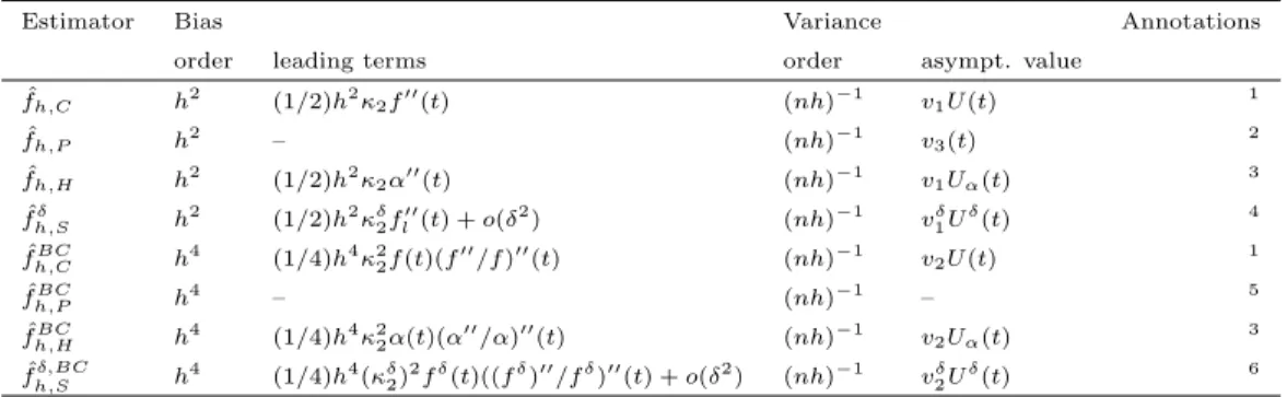
point-wise asymptotics. The asymptotic orders and the main terms of the point-wise asymptotic bias and variance of every estimator in this paper are given in Table 1 for T = 1. The results hold under usual
375
regularity conditions (see references).
We use the following notations in Table 1: κ2 = R1 −1s 2K(s)ds; κδ 2 = R1 −1s 2K(s)dµδ(s); U(t) = {nhγ(t)}−1f(t)F(t);Uδ(t) ={nhγδ(t)}−1fδ(t)Fδ(t) =U(t)+o(1);U α(t) ={nhγ(t)}−1α(t);v1= R K2(s)ds; vδ 1 = R K2(s)dµδ(s) = v 1+o(1); v2 = R Γ2 K(s)ds, with ΓK(s) = 2K−(K∗K)(s); v2δ = R Γ2 K(s)dµ(s) = v2+o(1);v3(t) = (R 1−t 0 w(t, s)f(t, s)ds) −2R1−t 0 w
2(t, s)f(t, s)dsfor the weightingw= (nh2)−1Pn
i=1Kb(z−
380
(Xi, Yi)),b= (h, h). The operator∗denotes convolution.
8. Simulation study
The focus of this paper is on the finite sample performance of the estimators we introduced in the pre-vious sections to show how useful they are in practice, especially to weed out unstable methods that are at risk of breaking down completely in challenging problems. The idea is to discover the best estimator among
385
our selection of density estimators whose bias terms are of the same asymptotic order and to find a rule of thumb for the number of observations that are necessary for the multiplicative bias correction to improve
Estimator Bias Variance Annotations
order leading terms order asympt. value
ˆ fh,C h2 (1/2)h2κ2f00(t) (nh)−1 v1U(t) 1 ˆ fh,P h2 – (nh)−1 v3(t) 2 ˆ fh,H h2 (1/2)h2κ2α00(t) (nh)−1 v1Uα(t) 3 ˆ fδ h,S h2 (1/2)h2κδ2f 00 l(t) +o(δ2) (nh) −1 vδ 1Uδ(t) 4 ˆ fBC h,C h4 (1/4)h4κ22f(t)(f 00/f)00(t) (nh)−1 v 2U(t) 1 ˆ fBC h,P h4 – (nh) −1 – 5 ˆ fBC h,H h4 (1/4)h4κ22α(t)(α 00/α)00(t) (nh)−1 v 2Uα(t) 3 ˆ fh,Sδ,BC h4 (1/4)h4(κδ2)2fδ(t)((fδ)00/fδ)00(t) +o(δ2) (nh)−1 vδ2Uδ(t) 6
Table 1: Main terms of point-wise asymptotic bias and variance terms under regularity assumptions. All bias and variance
terms contain an additional error of lower ordero(h2) oro(h4), respectively. The symbol “–” denotes that there is no closed
form solution.
Annotations: 1see Nielsen et al. (2009);2no closed form solution for bias, see Mammen et al. (2015);3asymptotic theory for
the hazard estimator ˆα and not for the resulting ˆfh,H, see Nielsen and Tanggaard (2001); 4Proposition 1, see notation in
Appendix A.1 ,δis width of histogram bins;5no closed form solution, see Mammen et al. (2015);6Proposition 2, see notation
in Appendix A.1 ,δis width of histogram bins.
bias. As pointed out in Section 7, the bias corrected estimators have a leading asymptotic bias term of order
O(h4) instead of O(h2), however, a higher order of convergence usually leads to larger bias for small finite
samples and the estimators behave differently despite their common order of convergence because of different
390
constants in the bias. Clearly, different performance can be due to pure noise as well and hence we run 1000 simulations for each estimation.
In four different settings on the unit square, i.e., for T = 1 we compare the best-case performance of all eight density estimators with respect to the integrated squared error
395
ISE( ˆfl, fl) =
Z 1 0
[ ˆfl(t)−fl(t)]2dt,
forl = 1,2. “Best-case” means that we choose the best possible bandwidth with respect to the ISE which can be calculated exactly since the true distribution is given. Hence, we avoid the problem of choosing a bandwidth given data.
For some of the estimators bandwidth selection has already been investigated. Mart´ınez-Miranda et al. (2013) apply the projection approach on real data and determine an optimal bandwidth for ˆfh,P and ˆfh,PBC by
400
cross-validation. The asymptotic behavior of bandwidths from cross-validation (see Rudemo (1982), Bow-man (1984) and Hall (1983)) and double one-sided cross-validation (DO-validation, see Hart and Yi (1998), Mart´ınez-Miranda et al. (2009)) for the counting process estimator ˆfh,C is given in Hiabu et al. (2016) where
the estimator is applied on data with a data-driven bandwidth. Cross-validation and DO-validation for the hazard estimator ˆαh,R that is used for the computation of ˆfh,H and full asymptotics of the resulting
405
bandwidths are given in G´amiz et al. (2016). However, data-driven bandwidth selection for the structured histogram approach and for the bias corrected versions of the counting process density and hazard estimators
are not covered yet in literature. In particular, a comparison of bandwidth selection results for the whole range of estimators in this study has not been done yet. Being beyond the scope of this paper, it will be part of future work.
410
The settings we chose are motivated by practical relevance in the application of actuarial reserving and by challenging distributions that point out weaknesses of the estimators.
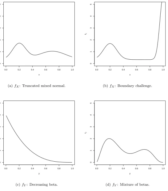
For f1 we take mixtures of truncated normal distributions. A mixture of N(0.2,0.1), N(0.5,3) and
N(0.7,0.2) with equal weights truncated to [0,1] is motivated by the empirical distributions of real data
415
sets and referred to as the “truncated mixed normal” distribution in the following. To make the estimation at the boundary more challenging, we have chosen a mixture of N(0.2,0.1), N(0.5,3) and N(1,0.05) with equal weights truncated to [0,1] as a variation and call it the “boundary challenge” distribution. Note that we try distributions forX with mass at the boundaries to investigate weaknesses because some estimators tend to values close to 0 at the edges. The issue of problems at the boundaries is well-known and local linear
420
kernel density estimators are known to perform better than local constant estimators, see e.g. Jones (1993). We investigate the following distributions for Y asf2. A beta distribution with parameters α= 1 and
β = 4 is taken as an empirically motivated “decreasing beta” distribution and we take a mixture of beta distributions with parameters (2,5), (3,10) and (9,4) and equal weights for a more complex example in which there are less observations with values ofY close to 0 and 1, respectively which results in less observations
425
in both corners of the triangleS1.
Withf2 decreasing towards 0 at the boundaries of the interval [0,1] in every investigated scenario, the
results in Table 3 reflect aforementioned problems of the estimation at boundaries: The ISE for f1 (which
always satisfiesf1(0), f1(1)>0) is much larger than that inf2 (withf2(0) =f2(1) = 0) in every single case.
The shapes of the probability density functions are given in Figure 1. We take all combinations of these
430
distributions and label the four scenarios in Table 2. For each scenario 1000 random samples of sizes 100, 1000 and 10000 were generated.
All simulated observations (Xi, Yi) satisfy Xi+Yi ≤ 1. Recalling the model in Section 2, this
right-truncation defines our observed subsetS1={(x, y)∈ S;x+y≤1} of the full supportS = [0,1]2 of (X, Y).
There are no observations in the complementS2= [0,1]2\ S1.
435
The interval [0,1] is discretized as a grid with 100 points and we take the corresponding approximation of the ISE. As mentioned in Section 5, we take the same bandwidthδ= 1/100 for the sieves estimators ˆfh,Sδ
and ˆfh,Sδ,BC.
We analyze two problems: First, we want to estimate the distributions ofX andY and we measure the results by the ISE in each component. The other problem is to estimate the massr=R
S2f(x, y)d(x, y) of the 440
distribution of (X, Y) inS2. We use the bandwidth minimizing the ISE for both problems since a bandwidth
Scenario Variable Distribution
1 X truncated mixed normal
Y decreasing beta
2 X boundary challenge
Y decreasing beta
3 X truncated mixed normal
Y mixture of betas
4 X boundary challenge
Y mixture of betas
Table 2: Scenarios in the simulation study.
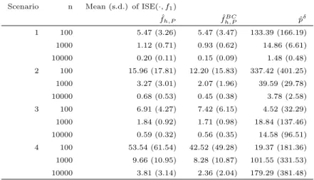
0.0 0.2 0.4 0.6 0.8 1.0 0 1 2 3 4 5 x fX
(a)fX: Truncated mixed normal.
0.0 0.2 0.4 0.6 0.8 1.0 0 1 2 3 4 5 x fX (b)fX: Boundary challenge. 0.0 0.2 0.4 0.6 0.8 1.0 0 1 2 3 4 5 y fY (c)fY: Decreasing beta. 0.0 0.2 0.4 0.6 0.8 1.0 0 1 2 3 4 5 y fY (d)fY: Mixture of betas.
the bottom left corner in the triangleS1— the area with the biggest impact on the estimate ofr. To find the
best bandwidth we compute the ISE for all bandwidthsh∈ {k/100 :k= 1,2, . . . ,50}and take the minimizer. Each kernel estimator is computed using the Epanechnikov kernelK(t) = 0.75(1−t2)I(−1≤t≤1),t∈[0,1].
445
For the projection estimatorsf1,h,P,f2,h,P, the algorithm stops afterkiterations if the criterion
1 m m X j=1 |f1(k)(sj)−f (k−1) 1 (sj)| f1(k−1)(sj) <0.001,
for the discretizations1, . . . , sm of [0,1] is fulfilled or if we have reached the defined maximum number of
k = 20 iterations. This method needs up to five times as long to be computed per bandwidth compared to the other estimators. The crucial part, however, is not the recursive algorithm, but the fact that being two-dimensional, it uses two-dimensional bandwidths. Fornh1 andnh2being the number of bandwidths that 450
are compared to estimate f1 and f2, respectively, the computation time of the two-dimensional estimator
is hence of computational orderO(nh1nh2) whereas the one-dimensional estimators have computation times
of orderO(nh1+nh2). Thus, the total computation time over all bandwidths is of much higher order than
that of the one-dimensional estimators.
8.1. Density estimation
455
The results of the comparison of the ISE are given in Table 3. In the sequel, the median and mean values of the ISE are always taken over 1000 simulation runs.
Our first observation is that the multiplicative bias correction works in practice. As indicated by the theoretical results, for a big enough number of observations the bias corrections result in a smaller bias than that of non-bias corrected estimators. Considering the ISE of both f1 and f2, there are only 4 out of 32
460
cases where the median bias of the non-corrected version of an estimator is better than its bias correction for a sample size of 10000 and those cases only occur in the challenging Scenarios 3 and 4. Three out of these four cases occur with the sieves estimator ˆfδ
h,S (with the ISE increased by less than 14% if we use bias
correction) and one with the hazard estimator ˆfh,H (where the bias correction is less than 5% worse with
respect to the ISE). Also measured by the empirical mean integrated squared error, there are only 4 out
465
of 32 cases where the bias correction does not work for sample size 10000. Here the crucial methods are the projection approach ˆfh,P in Scenario 2 and the ˆfh,Sδ in Scenarios 3 and 4. Besides, this indicates that
challenging estimation problems increase the number of observations that are needed for asymptotic bias improvements to show. For 25 out of 32 cases the bias correction is already better for 1000 observations in the median and in the empirical mean. Here, the observation can be made in all four approaches and in all
470
Scenario Estimator n = 100 n = 1000 n = 10000 ISE( · , f1 ) ISE( · , f2 ) ISE( · , f1 ) ISE( · , f2 ) ISE( · , f1 ) ISE( · , f2 ) Median Mean (s.d.) Median Mean (s.d.) Median Mean (s.d.) Median Mean (s.d.) Median Mean (s.d.) Median Mean (s.d.) 1 ˆfh,C 5.63 6.50 (3.73) 0.98 1.92 (2.49) 1.04 1.18 (0.65) 0.28 0.40 (0.39 ) 0.18 0.20 (0.10) 0.07 0.09 (0.06) ˆf B C h,C 5.93 7.10 (4.49) 1.91 3.09 (3.47) 1.03 1.17 (0.63) 0.17 0.28 (0.31 ) 0.15 0.17 (0.09) 0.02 0.04 (0.04) ˆfh,P 4.80 5.47 (3.26) 0.89 2.09 (2.88) 0.94 1.12 (0.71) 0.22 0.38 (0.44 ) 0.17 0.20 (0.11) 0.06 0.08 (0.07) ˆf B C h,P 4.69 5.47 (3.47) 1.23 2.11 (2.55) 0.77 0.93 (0.62) 0.10 0.17 (0.21 ) 0.12 0.15 (0.09) 0.02 0.04 (0.04) ˆfh,H 5.88 6.72 (4.08) 18 .99 20.24 (7.51) 1.35 1.49 (0.75) 7.97 8.15 (1.85 ) 0.38 0.40 (0.13) 5.15 5.16 (0.53) ˆf B C h,H 4.32 5.37 (3.68) 16 .02 17.32 (7.05) 1.03 1.14 (0.52) 6.72 6.88 (1.74 ) 0.32 0.33 (0.10) 4.72 4.74 (0.51) ˆf δ h,S 4.86 5.67 (4.01) 2.55 3.91 (3.72) 0.95 1.17 (0.81) 0.67 0.82 (0.57 ) 0.18 0.20 (0.11) 0.17 0.18 (0.09) ˆf δ ,B C h,S 5.04 6.28 (4.94) 1.27 2.33 (2.67) 0.88 1.10 (0.80) 0.50 0.63 (0.45 ) 0.14 0.16 (0.10) 0.13 0.15 (0.08) 2 ˆfh,C 12.54 18.96 (18.19) 0.88 1.7 6 (2.37) 3 .03 3.9 2 (3.17) 0 .27 0.40 ( 0 .41) 0.60 0.81 (0.64) 0.07 0.09 (0.06) ˆf B C h,C 12.09 18.19 (18.31) 1.62 2.8 0 (3.58) 2 .95 3.5 3 (2.62) 0 .17 0.28 ( 0 .31) 0.44 0.73 (0.80) 0.02 0.03 (0.03) ˆfh,P 9.39 15.96 (17.81) 0.50 1.18 (1.79) 2.39 3.27 (3.01) 0.08 0.12 (0.14 ) 0.51 0.68 (0.53) 0.03 0.03 (0.02) ˆf B C h,P 6.29 12.20 (15.83) 0.98 1.69 (2.17) 1.55 2.07 (1.96) 0.11 0.17 (0.17 ) 0.31 0.45 (0.38) 0.02 0.04 (0.04) ˆfh,H 11.01 16.46 (16.59) 19.20 20.3 4 (7.56) 2 .90 3.77 (2.74) 8 .00 8.17 ( 1 .87) 0.75 0.94 (0.66) 5.17 5.19 (0.56) ˆf B C h,H 9.58 15.58 (16.46) 15 .62 16.94 (6.93) 2.77 3.42 ( 2 .41) 6.64 6.84 (1.76 ) 0.56 0.78 (0.69) 4.76 4.77 (0.53) ˆf δ h,S 20.99 29.27 (24.99) 2.49 3.6 1 (3.49) 2 .85 5.01 (5.62) 0 .6 5 0.82 ( 0 .59) 0.45 0.78 (0.88) 0.16 0.18 (0.10) ˆf δ ,B C h,S 17.03 25.91 (24.32) 1.16 2.0 8 (2.39) 2 .18 4.08 (4.86) 0 .4 8 0.62 ( 0 .48) 0.32 0.56 (0.67) 0.13 0.15 (0.08) 3 ˆfh,C 8.67 10.05 ( 6.17) 6 .59 8.13 (6.05) 2.22 2.58 (1.52) 1.06 1.20 (0.68) 0.54 0.62 (0.40) 0.28 0.29 (0.10) ˆf B C h,C 8.74 11.45 (11.09) 6.97 8.93 (7.65) 2.00 2.42 (1.56) 1.06 1.24 (0.76 ) 0.41 0.49 (0.33) 0.19 0.20 (0.10) ˆfh,P 6.07 6.91 ( 4.27) 4.61 5.58 (4.45) 1.72 1.84 (0.92) 0.87 0.99 (0.58 ) 0.52 0.59 (0.32) 0.26 0.28 (0.10) ˆf B C h,P 5.98 7.42 ( 6.15) 5.00 6.14 (4.95) 1.51 1.71 (0.98) 0.90 1.01 (0.57 ) 0.48 0.56 (0.35) 0.19 0.20 (0.08) ˆfh,H 9.87 11.64 ( 7.84) 7 .11 8.59 (6.56) 2.95 3.30 (1.81) 1.61 1.75 (0.81) 0.85 0.98 (0.51) 0.57 0.58 (0.15) ˆf B C h,H 6.99 9.42 (11.26) 5 .97 7.96 (7.50) 1.73 2.00 (1.13) 1.20 1.39 (0.80) 0.57 0.62 (0.25) 0.42 0.44 (0.14) ˆf δ h,S 6.53 7.60 ( 5.62) 6.47 7.82 (5.53) 1.91 2.93 (4.25) 1.33 1.48 (0.74 ) 0.49 0.94 (2.33) 0.32 0.33 (0.11) ˆf δ ,B C h,S 7.37 9.21 ( 7.50) 6.69 8.08 (5.73) 1.99 3.21 (5.13) 1.45 1.56 (0.69 ) 0.50 0.97 (2.72) 0.36 0.37 (0.11) 4 ˆfh,C 37.08 66.06 (61.73) 6.16 7.0 8 (4.73) 6 .75 12.76 (14.90) 0 .94 1.04 ( 0 .53) 2.77 3.32 ( 2.87) 0.27 0.28 (0.10) ˆf B C h,C 33.33 62.84 (59.47) 6.40 7.6 5 (5.49) 6 .71 10.65 (12.53) 0 .90 1.04 ( 0 .57) 2.73 3.09 ( 2.11) 0.17 0.19 (0.09) ˆfh,P 17.31 53.54 (61.54) 3.96 4.7 2 (3.37) 6 .10 9.66 (10.95) 0.72 0.81 (0.44) 2.84 3.81 ( 3.14) 0.24 0.25 (0.09) ˆf B C h,P 13.73 42.52 (49.28) 4.44 5.2 5 (3.70) 4 .62 8.28 (10.87) 0.78 0.88 (0.49) 1.80 2.36 ( 2.04) 0.17 0.19 (0.08) ˆfh,H 27.47 62.02 (61.13) 6.63 7.5 7 (4.95) 7 .68 12.39 (13.47) 1 .4 6 1.57 ( 0 .69) 2.78 3.42 ( 2.42) 0.55 0.56 (0.14) ˆf B C h,H 26.81 50.81 (49.75) 5.34 6.6 4 (5.09) 6 .89 10.14 (11.39) 1 .0 8 1.19 ( 0 .59) 2.90 3.40 ( 2.32) 0.40 0.42 (0.13) ˆf δ h,S 99.38 95.48 (47.72) 5.96 6.8 3 (4.25) 29.70 35.93 (28.16) 1.18 1.30 (0.60) 9.54 13.13 (12.09) 0.30 0.31 (0.10) ˆf δ ,B C h,S 94.17 94.17 (56.06) 6.04 7.01 (4.44) 22.98 32.08 (28.29) 1.26 1.37 (0.57) 7.20 10.71 (10.33) 0.34 0.35 (0.10) T able 3: Median, mean and standard deviation of ISE( ˆf1 , f1 ) and ISE( ˆf2 , f2 ) for 100, 1000 and 1000 0 observ ations. The statistics are tak en o v er 1000 sim ulation runs for eac h setting and the ISE w as ev aluated on the same grid with 100 p oin ts whic h w as used b efore.
The second observation is that the two-dimensional estimators ˆfh,P and ˆfh,PBC globally perform best for
small samples sizes of not more than 10000. Especially for very small sample sizes (<1000) it outperforms the other estimators with and without bias correction. There is only one out of 32 cases where the best estimator for 100 observations is neither ˆfh,P nor ˆfh,PBC measured by median and only two cases measured
475
by the mean. Besides, it also competes well with the other three approaches for sample sizes of 1000 and 10000. However, with increasing sample sizes, the counting process estimator ˆfh,C and especially its bias
corrected version ˆfBC
h,C leads to the best results with respect to the integrated squared error in one of the four
scenarios. For even larger samples sizes (n= 106,107) which we investigated but which are not illustrated
here, the bias corrected one-dimensional counting process estimator performed best.
480
The sieves estimators ˆfh,Sδ , ˆfh,Sδ,BC perform surprisingly well and lead to satisfying results except for a complete breakdown in the estimation off1 with only 100 observations in Scenarios 2 and 4 which contain
the boundary challenge problem. However, in most cases, the counting process approach or the projection approach leads to a smaller ISE than both sieves estimators.
As expected, globally the hazard estimators ˆfh,H and ˆfh,HBC can’t compete either with the two best
485
approaches since the transformation from a hazard to a density function is not stable enough. Especially for the decreasing beta distribution in Scenarios 1 and 2 the hazard estimators failed at estimatingf2. However,
they perform well and they can compete with the other estimators in Scenarios 3 and 4 and especially in the estimation off1 for small sample sizes.
In contrast to the hazard estimators, all other estimators perform extraordinary in Scenarios 1 and 2
490
with respect to the estimation of f2, the mixed beta distribution. For the non-hazard estimators, Scenario
4 with the combination of the boundary challenge distribution and the mixture of beta distributions the estimation of f1 is the most challenging estimation problem with by far the biggest ISE throughout and
especially forn= 100 observations. The “boundary challenge” distribution also leads to slightly bigger ISE inf1in Scenario 2. In Scenario 1 we achieve the best results in the estimation of the distribution of X.
495
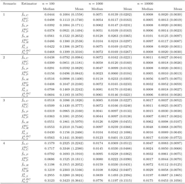
8.2. Application: Aggregated forecast
The main application we compare here is based on the estimation of the probability mass of the distri-bution of (X, Y) in the unobserved regionS2, i.e., we investigate an estimator
ˆ r( ˆf1,fˆ2) = Z S2 ˆ f1(x) ˆf2(y)d(x, y). ofr=RS
2f(x, y)d(x, y). Recall that we assumef(x, y) =f1(x)f2(y). Therefore, we estimatef(x, y) inrby
ˆ
f1(x) ˆf2(y). However, we are particularly interested in the estimation of the ratio between the probability
500
mass inS2 and that inS1, weighted by the number of observations, i.e., in the objectRn=nr/(1−r). We
estimateRn by ˆ Rn( ˆf1,fˆ2) = nˆr( ˆf1,fˆ2) 1−rˆ( ˆf1,fˆ2) .
Following the interpretation of the survival analysis approach, we want to know how many events will occur in the future, given the number of events in the past. This is illustrated through our main application of actuarial reserving mentioned in Section 1:
505
Example 1 (Reserving in non-life insurance; IBNR numbers). One has observed n past claims (Xi, Yi),
i = 1, . . . , n, where Xi denotes the year the accident of claim i happened and Yi is the delay until it was
reported to the insurance company. We want to estimate the number of claims for accidents that have already happened but will be reported in the future. The density of (X, Y)is assumed to bef andX andY
are independent.
510
The data fits into the triangular form of Section 2, since by assumption all observations ofX occurred less thanT years ago. The time of data collection is represented by the diagonal on the scaled squareS= [0, T]2 since only claims that have incurred and that also have been reported before that day are observed.
In our model, and in particular assuming a maximum delay ofT years, there is an unknown total number of claims but we know that all claims are contained in the squared support [0, T]2. Hence, an estimate for
515
the number of outstanding claims isRn, the ratio of the probability of a claim to be in the future divided by
the probability of already being observed times the number of observationsn that are already observed. Another direct application would be the estimation of the RBNS claims, the claims that have been reported but not yet settled, i.e., the final payments have not been made yet for these claims.
Another good illustration is given through aforementioned medical study.
520
Example 2 (Medical study). Study about patients who go infected with a deadly disease during the lastT
years. Assuming patients are only included into the data set after their deaths, one wants to forecast the total number of deaths in the next years not knowing the number of infected people. We only assume the time until death Y is at mostT years and we have data about the time of death(Xi+Yi)and time of infection
(Xi)of npatients (i= 1, . . . , n) that have died during the lastT years. The number of future deaths in this
525
group of people is then given byRn if time until death and time of infection are independent with densities
f1 andf2, respectively. 3
The estimated probability mass ˆr( ˆf1,fˆ2) just depends on the marginal estimators ˆf1,fˆ2. However, in
many cases estimates ofRn are more accurate than density estimators since errors can “cancel each other
out”. In practice, over-smoothed density estimator often lead to a more stable estimation of this number.
530
Because of the practical relevance of this estimation problem, we hence also use the fit of ˆRn as a measure
of goodness for our estimators.
To compare the approaches, we use the relative error err( ˆf1,fˆ2) =
ˆ
Rn( ˆf1,fˆ2)−Rn
Rn
,
The results of the estimation of Rn are given in Table 4. We state the median, mean and standard
535
deviation of err2in the 1000 simulation runs.
Here, clearly the bias corrected version ˆfBC
h,P of the projection estimator can be recommended as an overall
winner. In ten of the twelve cases, it is the best estimator ofRn in the mean integrated squared error. The
regular projection estimator ˆfh,P performed best in two cases (in one of which ˆfh,P and ˆfh,PBC have the same
error) and the bias corrected counting process estimator ˆfBC
h,C wins in one of the twelve cases. The results
540
for the median are the same except for one case where ˆfh,C slightly outperforms ˆfh,CBC.
In two thirds of the scenarios the best three estimators for the reserve measured by the median arise from the counting process and the projection approach. A sieves estimate only ranks second or twice in four cases whereas the hazard estimators only rank third in two cases. Therefore, it seems clear that the method of sieves is not smoothed enough, and that the hazard estimation approach is the wrong transformation of the
545
unknown one-dimensional functions for in-sample forecasting. We are therefore left with the projected density approach and the backward survival density approach as our two test winners for in-sample forecasting. In the next section, we will further illustrate why the method of sieves might be too simple and why modern smoothing approaches are indeed necessary when working with in-sample forecasting problems. This is not an established fact or a well-known insight. For example, in the excellent book Martinussen and Scheike
550
(2006) the point of view has been taken to concentrate estimation on integrated quantities that can be estimated without smoothing at√n-rates of convergence. While this obviously simplifies a lot of things in many important cases and without harming the applied statistician when interpreting results, this point of view does not seem to work when considering in-sample forecasting. There is more information on this in the next section.
555
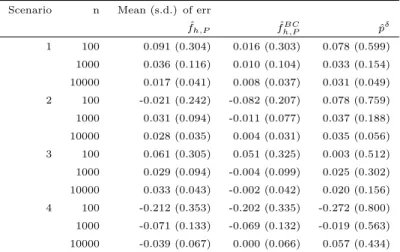
8.3. Necessity of smoothing in the aggregated forecast
To illustrate the importance of smoothing in the estimation problem in the last section, we compare the results of ˆfh,P and ˆfh,PBC (which we have identified as the estimators from the most promising approach) with
the discrete non-smoothed histogram estimator ˆpδ which is widely used in practice in the insurance industry,
the so-called chain ladder estimators for the actuarial reserve. It occurs in the application explained in the
560
last section and it is derived from the forward factors mentioned in Section 5 as explained in e.g. England and Verrall (2002).
The method only uses the accumulation in the direction ofX as given by the formulas in Section 5. The development factors ˆλj are used to extrapolate forecasts for the values of the cumulative matrix D in the
unobserved region via ˆ
Di,n−i+2=Di,n−i+1λˆn−i+2,
ˆ
Scenario Estimator n= 100 n= 1000 n= 10000
Median Mean Median Mean Median Mean
1 fˆh,C 0.0444 0.1004 (0.1558) 0.0071 0.0139 (0.0202) 0.0008 0.0020 (0.0030) ˆ fBC h,C 0.0498 0.1113 (0.1740) 0.0054 0.0117 (0.0163) 0.0005 0.0013 (0.0019) ˆ fh,P 0.0392 0.1004 (0.1711) 0.0062 0.0147 (0.0231) 0.0008 0.0020 (0.0030) ˆ fBC h,P 0.0378 0.0921 (0.1494) 0.0051 0.0109 (0.0163) 0.0006 0.0014 (0.0023) ˆ fh,H 0.0561 0.1522 (0.2652) 0.0128 0.0263 (0.0365) 0.0101 0.0125 (0.0097) ˆ fBC h,H 0.0486 0.1380 (0.2538) 0.0104 0.0218 (0.0297) 0.0097 0.0117 (0.0087) ˆ fδ h,S 0.0422 0.1306 (0.2873) 0.0075 0.0169 (0.0274) 0.0008 0.0020 (0.0031) ˆ fh,Sδ,BC 0.0468 0.1399 (0.3316) 0.0072 0.0169 (0.0267) 0.0008 0.0020 (0.0030) 2 fˆh,C 0.0438 0.0792 (0.0984) 0.0072 0.0162 (0.0221) 0.0011 0.0027 (0.0044) ˆ fBC h,C 0.0399 0.0851 (0.1181) 0.0058 0.0120 (0.0160) 0.0008 0.0018 (0.0026) ˆ fh,P 0.0291 0.0592 (0.0829) 0.0047 0.0099 (0.0132) 0.0008 0.0020 (0.0031) ˆ fBC h,P 0.0156 0.0496 (0.0843) 0.0023 0.0060 (0.0104) 0.0005 0.0010 (0.0013) ˆ fh,H 0.0516 0.0998 (0.1400) 0.0118 0.0233 (0.0305) 0.0056 0.0075 (0.0075) ˆ fBC h,H 0.0408 0.1047 (0.2160) 0.0072 0.0165 (0.0233) 0.0032 0.0052 (0.0059) ˆ fδ h,S 0.0708 0.1469 (0.2242) 0.0081 0.0170 (0.0246) 0.0008 0.0018 (0.0027) ˆ fh,Sδ,BC 0.0604 0.1183 (0.1670) 0.0061 0.0146 (0.0221) 0.0006 0.0016 (0.0026) 3 fˆh,C 0.0518 0.1086 (0.1826) 0.0085 0.0168 (0.0227) 0.0017 0.0037 (0.0052) ˆ fBC h,C 0.0509 0.1430 (0.3777) 0.0072 0.0166 (0.0246) 0.0011 0.0025 (0.0037) ˆ fh,P 0.0319 0.0965 (0.2160) 0.0041 0.0097 (0.0133) 0.0015 0.0030 (0.0038) ˆ fBC h,P 0.0363 0.1081 (0.2558) 0.0044 0.0097 (0.0138) 0.0007 0.0017 (0.0024) ˆ fh,H 0.0551 0.1861 (0.5970) 0.0126 0.0299 (0.0455) 0.0062 0.0098 (0.0107) ˆ fBC h,H 0.0553 0.2310 (0.7446) 0.0097 0.0239 (0.0366) 0.0048 0.0068 (0.0070) ˆ fδ h,S 0.0430 0.1156 (0.2466) 0.0104 0.0342 (0.1006) 0.0016 0.0089 (0.0649) ˆ fh,Sδ,BC 0.0563 0.1441 (0.3040) 0.0123 0.0401 (0.1225) 0.0017 0.0100 (0.0772) 4 fˆh,C 0.1579 0.2325 (0.2242) 0.0174 0.0369 (0.0512) 0.0047 0.0083 (0.0097) ˆ fBC h,C 0.1717 0.3348 (1.2380) 0.0145 0.0330 (0.0488) 0.0024 0.0050 (0.0068) ˆ fh,P 0.0792 0.1693 (0.1910) 0.0095 0.0228 (0.0362) 0.0032 0.0061 (0.0075) ˆ fBC h,P 0.0686 0.1525 (0.1811) 0.0080 0.0222 (0.0390) 0.0017 0.0044 (0.0070) ˆ fh,H 0.1198 0.1915 (0.2052) 0.0159 0.0330 (0.0431) 0.0072 0.0112 (0.0125) ˆ fBC h,H 0.1219 0.2303 (0.5166) 0.0108 0.0262 (0.0407) 0.0029 0.0058 (0.0078) ˆ fδ h,S 0.2955 0.3260 (0.3824) 0.0839 0.1493 (0.2394) 0.0197 0.0687 (0.1865) ˆ fh,Sδ,BC 0.3123 0.3423 (0.3641) 0.0776 0.1197 (0.1515) 0.0175 0.0453 (0.1056)
Table 4: Median, mean and standard deviation of the squared relative errors err2 for 100, 1000 and 10000 observations. The
statistics are taken over 1000 simulation runs for each setting.
The forecast for Rn, i.e., the so-called actuarial reserve in aforementioned application, is then given by
the aggregated estimated data:
565 ˆ RCLMn = X i+j>n ˆ Di,j,
where the summation is over all valid indicesi, j= 1, . . . , n such thati+j > n.
The relative errors err of the results are given in Table 5. In nine out of twelve cases, the bias corrected projection estimators ˆfBC
h,P lead to the smallest absolute error in the estimation ofRn whereas the non bias
corrected ˆfh,P scored best once. Although the discrete chain ladder method has the smallest absolute error
570