Evaluation of Classifier Complexity for Delay
Tolerant Network Routing
Rachel Dudukovich Flight Software Branch NASA Glenn Research Center
Cleveland, OH 44135 [email protected]
Gilbert Clark
Secure Networks, System Integration and Test Branch
NASA Glenn Research Center Cleveland, OH 44135 [email protected]
Christos Papachristou Electrical, Computer, and Systems
Engineering
Case Western Reserve University Cleveland, OH 44106
Abstract — The growing popularity of small cost-effective satellites (SmallSats, CubeSats, etc.) creates the potential for a variety of new science applications involving multiple nodes functioning together to achieve a task, such as swarms and constellations. As this technology develops and is deployed for missions in Low Earth Orbit and beyond, the use of delay tolerant networking (DTN) techniques may improve communication capabilities within the network. In this paper, a network hierarchy is developed from heterogeneous networks of SmallSats, surface vehicles, relay satellites and ground stations which form an integrated network. There is a trade-off between complexity, flexibility, and scalability of user defined schedules versus autonomous routing as the number of nodes in the network increases. To address these issues, this work proposes a machine learning classifier based on DTN routing metrics. A framework is developed which will allow for the use of several categories of machine learning algorithms (decision tree, random forest, and deep learning) to be applied to a dataset of historical network statistics, which allows for the evaluation of algorithm complexity versus performance to be explored. We develop the emulation of a hierarchical network, consisting of tens of nodes which form a cognitive network architecture. CORE (Common Open Research Emulator) is used to emulate the network using bundle protocol and DTN IP neighbor discovery.
Keywords—Delay tolerant networking, machine learning, opportunistic routing, feature engineering, autoencoders
I. INTRODUCTION
The research areas of Delay Tolerant Networking (DTN) [1] and cognitive communications can be combined to improve quality of service, throughput (or goodput), and reduce operations costs for a variety of aerospace communication applications. This work explores the trade-offs for three different algorithmic approaches to apply machine learning to the task of opportunistic routing in a DTN, as well as other related networks such as mobile ad hoc networks (MANETS) and wireless sensor networks (WSN). Section I introduces the topic and provides a brief summary of delay tolerant networking. Section II, Problem Formulation, discusses the network architecture concept, the development of the dataset and feature vector. The complexity in terms of training times, required number of training examples, and handcrafted feature engineering are discussed for the selected methods of decision tree, random forest, and a neural network based autoencoder. Section III discusses the experimental emulation set up, the
software tools used for the emulation, and emulation parameters. Section IV discusses the metrics used for the classifier performance evaluation, DTN routing metrics, and preliminary results. Section V concludes the paper with final comments and future work.
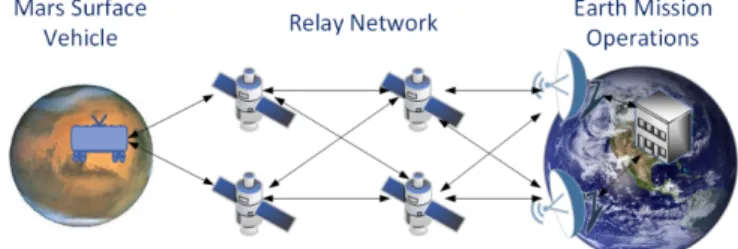
Fig. 1 shows an example of a multi-hop network to demonstrate the routing problem studied in this paper. A deep space surface vehicle or other similar research asset transmits science data to orbiting satellites. There may be varying periods of accessibility from the surface vehicle to each relay as well as differing data rates for each link. Once data is transmitted to the orbiter satellites, they will transmit their data to a network of communication relay satellites. The relay satellites will forward the data to one of several available earth ground stations. In addition, though not shown in this picture for simplicity, the deep space surface vehicles as well as orbiter satellites may transmit data directly to earth. Typically, these direct to earth connections may be much slower when compared to the relay network.
Figure 1. Multi-hop Network Example
A. Delay Tolerant Networking
The NASA SCaN networks currently consist of the Near Earth Network (NEN), the Space Network (SN) and the Deep Space Network (DSN) [2]. Within these networks, a variety of different protocol stacks are used. These protocols are intended to satisfy diverse requirements for specific environments. Roundtrip times may vary from less than a second for communication from Low Earth Orbit to Earth and up to 45 minutes from the Earth surface to Mars [3]. Common protocol mechanisms such as acknowledgements can negatively impact performance and throughput for this type of deep space scenario.
Figure 2. Bundle Protocol Network Stack Example [6]
The DTN architecture [1] and the Bundle Protocol (BP) [4] address the issues of heterogeneous network stacks as well as long periods of disconnection or unreliable contact. The Bundle Protocol uses a store and forward technique to mitigate these disruptions. Data will be stored when the network becomes unavailable and transmitted once connectivity is restored. Data can be transmitted to a destination without a known end-to-end path by relaying to nodes which may eventually come in contact with the destination. The Bundle Protocol creates an additional layer between the application layer and underlying transport, datalink, and physical layers within the protocol stack. This overlay concept abstracts away the differences in lower level details so that nodes may use a variety of different protocols from the transport to physical layers as appropriate for their particular conditions.
Fig. 2 shows an example of the various protocols that could be used in a delay tolerant network consisting of a landed Martian rover, orbiter satellite, and various components of the ground segment needed to reach a science mission's control center. Nodes in close proximity together on a planet's surface may use a standard TCP based network. Long distance links such as a Mars relay to Earth may use protocols designed for extended distances such as the Licklider Transmission Protocol (LTP) [5]. The bundle layer will abstract away these differences, which will be handled by the lower level mechanisms. The bundle layer will be concerned with storage of the data until an appropriate transmission time, custody transfer of the data and routing of the data.
B. Hierarchical Network Architecture
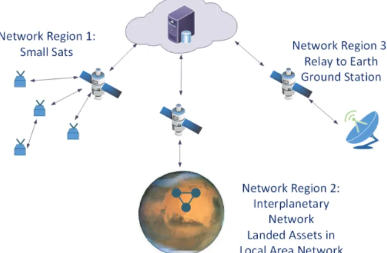
In the routing problem studied in this paper, the network consists of a set of small mobile nodes which send data to one or more potential relay satellites or data mules. A set of “worker nodes,” such as SmallSats, picosatellites, CubeSats, etc. perform a series of tasks such as image collection or various sensing applications. Within the network there is one or more central nodes which can be used to store, process, and relay data. This alleviates the need for extensive data storage and processing capacity on the smaller nodes. Arslan et al. [7] develop such an architecture focused on the use of picosatellites which acts a constellation to complete tasks currently done by large multifunctional satellites. The network forms a hierarchical structure with small mobile nodes at the lowest level, relay satellites at the intermediate level, and the ground
segment on earth as the top level of the network structure. In this work we propose that this architecture also lends itself toward implementing supervised and unsupervised learning methods that will allow for intelligent data routing and node self-organization. Fig. 3 shows an example of this concept.
Figure 3. Hierarchical Network Example
The network hierarchy allows for a large amount of data to be stored from multiple nodes and to create a more complete picture of the network. This centralization allows for the use of powerful processors and graphics processing units which would be impractical on very resource constrained nodes such as picosatellites and SmallSats. This method allows more data to be available to the learning algorithm, does not require constant communication between the central node and worker nodes, and allows algorithms to be trained offline and simply deploy the trained model to each worker node.
II. PROBLEM FORMULATION
There are three main issues we will focus on in terms of the complexity of each learning method. They are the amount of training data required to successfully construct a reasonable representation of the network, the amount of time spent on feature engineering and data preparation, and the training time required for each algorithm. We do not consider the processing time for prediction on each node that the routing algorithm will be deployed on since the model will be trained prior to deployment and each solution can be simplified into a series of source, destination, current time, and preferred neighbor tuples. A. Training Times
The simplest method we explore is the ID3 decision tree. Decision trees construct a graph like tree structure based on a series of yes or no decision criteria as learned by associating frequency of occurrences of a specific label value with a specific attribute value. The ID3 decision tree algorithm uses information gain, a function based on the entropy of a training data set to determine which attributes should be used as the root decision of the tree, following down through the lower branches of the tree [8]. Information gain is used to determine the relevance of each variable to predicting the category label; it is
the amount of information gained about the label from observing a specific attribute. The attribute which has the greatest information gain is selected as the root node, and is then evaluated recursively to generate the rest of the tree structure. The complexity of a decision tree with n attributes and m training samples is O(n×m log m) [9].
The next method we explore is the random forest algorithm [10]. The random forest is an ensemble of decision trees. A detailed analysis of the model is given in [11]. Intuitively, an estimate for the complexity of a random forest can be given by O(M(n×m log m)), where again n is the number of attributes in each tree, m is the number of samples and M is the number of trees created.
Finally, we develop an autoencoder to attempt to determine relevant features from the network data without the need for extensive manual feature engineering. Autoencoders attempt to reconstruct their input data set by developing encoding and decoding functions that minimize the error between the input data and reconstructed data. While it is more complicated to determine the complexity of the algorithm, we estimate the training complexity to be O((N+F)DI), where F is the dimension of the node feature vector, N is the number of nodes, D is the size of the hidden layer, and I is the number of iterations [12].
B. Sample Size
There is a trade-off between analyzing large amounts of data in hopes of increasing model accuracy versus the amount of processing time and associated costs. While the volume of training data available does impact model performance, the number of variables within the dataset also has a significant impact on the selected analysis method. Data mining and machine learning techniques provide insight into complex relationships between variables beyond merely processing large volumes of data. Indeed, decision tree based methods are known to be subject to over-fitting with large amounts of data. A variety of pruning algorithms have been developed to compensate for this problem. Morgan et al. [13] note that decision tree accuracy increases with sample size, attaining performance within 0.5 percent of terminal accuracy often with datasets of the order of 10,000 samples.
C. Feature Engineering and Problem Formulation
While decision trees and the ensemble approach of random forests are intuitive to understand for basic problems, the success of the algorithm largely depends on what features have been selected for the model. In previous work, we developed a multi-label approach which aims to reconstruct satisfactory routing paths based on the feature vector of the source node id, the neighboring node in question for forwarding, the destination node, and the current time [14]. This method essentially takes into account the frequency or count of messages successfully delivered based on which nodes they had visited and at what time.
The drawback of this method is that there many additional variables that impact the network and routing performance that are not taken into account. Information such as the physical location of the node can be utilized as a feature using
unsupervised techniques such as clustering [15]. Additional information such as the bundle delivery ratio per node, the number of retransmissions or failed attempts, and the delivery delay are not taken into account. While delivery delay may seem to be the best performance indictor in many traditional networking scenarios, this does not hold for delay tolerant networks. The delay may be a characteristic of the network itself such as a variable round trip time based on current location in an orbit, or unrelated disruptions. Therefore the correlation with algorithm performance and delivery delay is not easily discernable. It is in this case that one of the many strengths of deep learning may be beneficial. Deep learning can be used to automate feature engineering, saving engineering time spent on determining relevant features in the data and formulating the problem based on patterns in the data that may be difficult to manually detect or represent.
III. EXPERIMENTAL IMPLEMENTATION
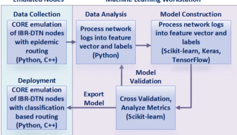
Fig. 4 shows the machine learning workflow as described in [16] and how it relates to the emulation process developed in this work. The learning phases consist of data collection, data analysis, model construction, model validation, and deployment.
The data collection phase is done using CORE (Common Open Research Emulator) [17]. CORE uses Linux containers to create light weight virtual machines that can run custom protocols, Python and shell scripts, and other programs just as any host machine would. IBR-DTN [18] is used as the DTN bundle agent on each node, utilizing the Bundle Protocol, TCP/IP convergence layer and DTN IP Neighbor Discovery (IPND). During the data collection phase, routing is done using epidemic routing [19]. Each node sends bundles at a specified interval to a list of randomly generated destinations. Logs are kept of when the bundles were sent, delivered, and which nodes each bundle was forwarded to.
Figure 4. Network emulation and learning workflow
The emulation consists of 20 nodes with the node radio range set to 250 m and the data rate is varied over emulations from 10 kbps to 1 Mbps. The nodes move on a grid based on pixel locations which correspond to longitude and latitude coordinates defined by the user. BonnMotion was used to create
the mobility scripts for each node based on the Random Walk mobility model [20]. BonnMotion is a suite of mathematical mobility models which build scenarios of a specified length of time in which object coordinates are varied according to the selected model. Object speed, boundary behaviors, coordinate scales, and many other parameters are configurable. These generated coordinates are translated to the CORE canvas and used for node position and link range determination. Fig. 5 shows a screen shot of the CORE emulation. The link between each node is green when communication is possible and disappears when the node moves out of range.
Figure 5. Subset of CORE Network Emulation
After the emulation has completed, the next phase in the workflow is data analysis. Logs of the network behavior are processed into the format of a feature vector and label. For this series of experiments, the feature vector consists of the bundle id, the source node number, destination node number, the current node in possession of the bundle, the node the bundle will be forwarded to, and an integer time index representing the current time period. The total emulation time is divided into one minute increments and this index indicates which minute this data was obtained from. This is done to turn the timestamp into a discrete feature for learning. Each of these feature vectors are labelled with a binary indicator representing if the bundle was ultimately delivered to the final destination or not. This is perhaps the simplest data format possible with the most limited amount of manual feature engineering, since in this experiment it is desired to see how each algorithm will determine the most important features in the data. The promise of using more complex models such as an autoencoder versus decision tree would be that the algorithm itself would eliminate the need for manual feature engineering.
The next step in our process is constructing the model. For these experiments the decision tree, random forest, and an autoencoder were each trained on the data set generated in the prior learning phase. This was done using Scikit-learn [21] for the decision tree and random forest, and Keras [22] and TensorFlow [23] for the autoencoder. Similarly, the model validation is done using K-fold cross validation and scoring metrics available in Scikit-learn. Once a satisfactory model is obtained, it is exported for use in a new emulation.
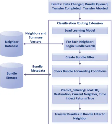
The final step in the workflow, deployment is done in a similar emulation as the data collection phase. However in this step, rather than using epidemic routing, a classification based routing extension is used. This routing extension uses the trained model to predict which neighbor is the most reliable neighbor to forward the bundle to base on the model delivery prediction. Fig. 6 shows a block diagram of the classification routing extension that has been developed in this work, based on IBR-DTN.
IBR-DTN, Instituts für Betriebssysteme und Rechnerverbund (Institute of Operating Systems and Computer Networks) Delay Tolerant Network, is a bundle protocol implementation developed at the Technical University of Braunschweig [18]. It is focused on minimizing resource consumption for embedded applications and uses an event based architecture. Routing extensions can be developed using C++ inheritance from a base router class. Various events within the node such as new bundles being queued or bundle transfer completed will trigger a new search for bundles to be sent to available neighbors. Summary vectors of bundles already known to neighboring nodes are maintained and used as filtering criteria for new bundles to be sent. This eliminates the transmission of many redundant bundles. Other criteria such as hop limits are also used in the bundle filter criteria. The algorithm employed in this work adds an additional filtering criteria based on the predicted likelihood of delivery.
IV. EVALUATION
The performance of the classification based routing method is evaluated in two steps. First the model itself must be evaluated using traditional machine learning metrics to determine if it is able to accurately predict bundle delivery based on the data set. After this is completed, the model is used in the routing extension and the overall performance is evaluated with DTN routing metrics.
Since the purpose of this work is to evaluate the tradeoff between simpler algorithms such as the decision tree, ensemble methods, or more complex deep learning methods, the first metric examined is the training time. Table I shows the average training time for each algorithm used.
TABLE I. MODEL TRAINING TIMES
Model Training Times
Algorithm Training Time (s)
Decision Tree 0.05 Random Forest,
depth 2 0.77
Autoencoder 323.36
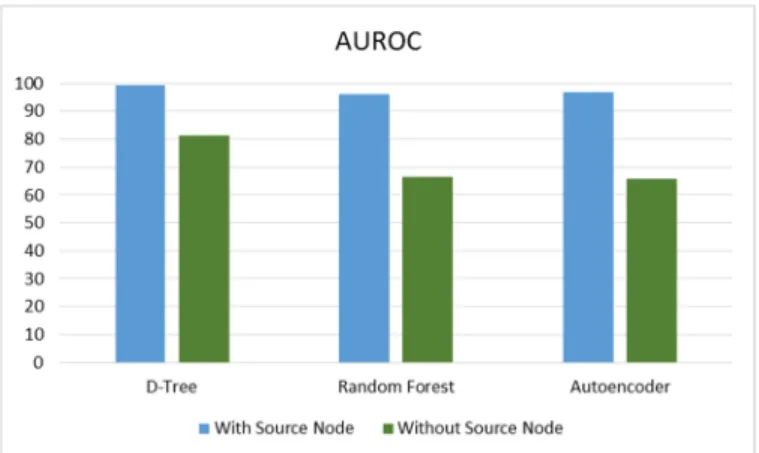
The machine learning metrics used to score each model were AUROC (Area Under Receiver Operating Characteristic) curve, accuracy, precision, recall, and F1 score. These metrics are typically considered unitless and written either as a ratio between 0 and 1, or a percentage from 0 to 100. In all cases, a larger value indicates better performance.
In addition, the most important features determined by each model were examined. It was found that the source node was the most important feature in the first series of tests. However, the source of a bundle does not supply any information on how the bundle should be forwarded, other than to avoid routing loops back to the original sender. It was decided to eliminate this feature, since it dominates the model without providing useful information. Another series of training and scoring was performed with the source node removed from the feature vector. The results are shown in Fig. 7 through 11. The blue metrics indicate training with the source feature and green indicates training without it. It can be seen that for their simplicity, decision trees perform acceptably well when compared to the random forest and the autoencoder, while having a much shorter training time. It should be noted that the set of features used in this example were quite simple and the use of additional features could further complicate the model and require more sophisticated methods.
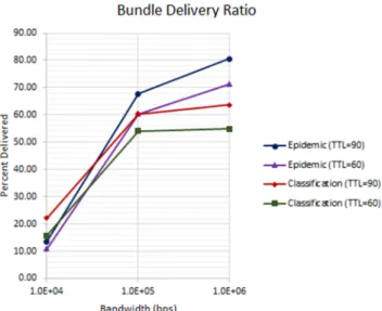
Finally the trained model is used in the classification routing extension and its results are compared to epidemic routing. It is expected that epidemic will have a higher bundle delivery ratio since in this instance, all bundles unknown to the neighboring node are replicated. The classification based routing method only replicates bundles when it predicts that the neighboring node will be associated with delivering the bundle to the final destination. This reduces the amount of unnecessary overhead and processing. Since fewer unneeded bundles occupy storage and transmissions queues, fewer bundles expire as compared to
epidemic routing. These results are shown in Fig. 12 and 13. The emulations were performed with varying node data rates and bundle time-to-live (TTL) in order to evaluate the impact on bundle expiration.
Figure 7. AUROC with and without source feature
Figure 8. Accuracy with and without source feature
Figure 10. Recall with and without source feature
Figure 11. F1 Score with and without source feature
Figure 12. Bundle Delivery Ratio
Figure 13. Bundles Expired
V. CONCLUSION
In summary, this work discusses some of the basic concepts and protocols of delay tolerant networking (DTN). A network architecture of relay nodes is described, with implications to the design of a cognitive network based on machine learning models in mind. Several common machine learning techniques (decision trees, random forest, and neural network autoencoder) are evaluated for use in an intelligent routing scheme. IBR-DTN was used as the base bundle protocol implementation and CORE was used to emulate the network. The emulated network serves to generate the learning dataset, as well as to test the classification based routing extension. Common machine learning metrics were used to score the trained model and DTN routing metrics were used to evaluate the routing extension performance. It was found that for this particular dataset, the simple decision tree based model performed sufficiently well. It is reasonable to suspect that this might not always be true when applied to more complex datasets.
In conclusion, for very simple features, basic machine learning methods may be sufficient for satisfactory performance when compared to more advanced deep learning models. The advantage of methods such as the autoencoder is that it eliminates the need for hand developed feature engineering in data where it may be difficult to determine what features are relevant.
For future work, we are interested in expanding our dataset with more information such as node location/position, buffer capacity, and retransmission attempts. This will perhaps provide a more complex model that will leverage the insight of deep learning models. In addition, other machine learning techniques can continue to be explored, such as reinforcement learning. A variety of techniques may prove to be better suited for a particular application and architecture.
REFERENCES
[1] V. Cerf, S. Burleigh, and K. Fall, “Delay-tolerant networking architecture,” https://tools.ietf.org/html/rfc4838, 04 2007.
[2] “Space Communications and Navigation (SCaN) Network Architecture Definition Document (ADD),” National
Aeronautics and Space Administration, Tech. Rep., 2014. [3] The Consultative Committee for Space Data Systems , “Cislunar space internetworking architecture,” The
Consultative Committee for Space Data Systems , Tech. Rep., 2006.
[4] K. Scott and S. Burleigh, “Bundle Protocol Specification,” https://tools.ietf.org/html/rfc5050, 2007. [5] M. Ramadas, S. Burleigh, and S. Farrell, “Licklider Transmission Protocol-Specification, RFC 5326,” https://-tools.ietf.org/html/rfc5326, 2008.
[6] The Consultative Committee for Space Data Systems, Rationale, Scenarios, and Requirements for DTN in Space, 2010.
[7] T. Arslan, et al., “Espacenet: A framework of evolvable and reconfigurable sensor networks for aerospace-based monitoring and diagnostics,” in First NASA/ESA Conference on Adaptive Hardware and Systems (AHS’06), June 2006, pp. 323–329.
[8] T. Mitchell, Machine Learning, C. I. Liu, Ed. McGraw-Hill, 1997.
[9] M. H. C. P. I. Witten, E. Frank, Data Mining: Practical Machine Learning Tools and Techniques, C. Kent, Ed. Morgan Kaufmann, 2011.
[10] L. Breiman, “Random forests,” Machine Learning, vol. 45, Oct. 2001.
[11] G. Biau, “Analysis of a random forests model,” J. Mach. Learn. Res., vol. 13, no. 1, pp. 1063–1095, Apr. 2012.
[12] P. V. Tran, “Learning to make predictions on graphs with autoencoders,” 2018 IEEE 5th International Conference on Data Science and Advanced Analytics (DSAA), pp. 237–245, 2018.
[13] J. Morgan, “Sample size and modeling accuracy of decision tree based data mining tools,” 2003.
[14] R. Dudukovich and C. Papachristou, “Delay tolerant network routing as a machine learning classification problem,” in Proceedings of The NASA/ESA Conference on Adaptive Hardware and Systems, Edinburgh, UK, 2018.
[15] R. Dudukovich, “Application of machine learning techniques to delay tolerant network routing,” Ph.D. dissertation, Case Western Reserve University, 2019. [16] M. Wang, et al., “Machine learning for networking: Workflow, advances and opportunities,” CoRR, vol. abs/1709.08339, 2017.
[17] J. Ahrenholz, “Comparison of CORE Network Emulation Platforms,” in Proceedings of the 2010 IEEE Military Communications Conference. IEEE, 2010, pp. 166–171. [18] J. Morgenroth, “IBR-DTN - A Modular and Lightweight Implementation of the Bundle Protocol,” https://github.com/-ibrdtn/ibrdtn.
[19] A. Vahdat and D. Becker, “Epidemic routing for partially-connected ad hoc networks,” 2000.
[20] “BonnMotion A Mobility Scenario Generation and Analysis Tool,” http://sys.cs.uos.de/bonnmotion/.
[21] F. Pedregosa, et al. , “Scikit-learn: Machine learning in Python,” Journal of Machine Learning Research, vol. 12, pp. 2825–2830, 2011.
[22] F. Chollet et al., “Keras,” https://keras.io, 2015. [23] M. Abadi, et al. “TensorFlow: Large-scale machine learning on heterogeneous systems,” 2015, software available from tensorflow.org. [Online]. Available: