Extending APEx (Accuracy-Aware Differentially Private Data Exploration) to Multiple Table Queries

Scholarship at UWindsor

Scholarship at UWindsor

Electronic Theses and Dissertations Theses, Dissertations, and Major Papers

10-30-2020

Extending APEx (Accuracy-Aware Differentially Private Data

Extending APEx (Accuracy-Aware Differentially Private Data

Exploration) to Multiple Table Queries

Exploration) to Multiple Table Queries

University of Windsor

Follow this and additional works at: https://scholar.uwindsor.ca/etd

Recommended Citation Recommended Citation

Singh, Karmanjot, "Extending APEx (Accuracy-Aware Differentially Private Data Exploration) to Multiple Table Queries" (2020). Electronic Theses and Dissertations. 8482.

https://scholar.uwindsor.ca/etd/8482

This online database contains the full-text of PhD dissertations and Masters’ theses of University of Windsor students from 1954 forward. These documents are made available for personal study and research purposes only, in accordance with the Canadian Copyright Act and the Creative Commons license—CC BY-NC-ND (Attribution, Non-Commercial, No Derivative Works). Under this license, works must always be attributed to the copyright holder (original author), cannot be used for any commercial purposes, and may not be altered. Any other use would require the permission of the copyright holder. Students may inquire about withdrawing their dissertation and/or thesis from this database. For additional inquiries, please contact the repository administrator via email

Differentially Private Data Exploration)

to Multiple Table Queries

By

Karmanjot Singh

A Thesis

Submitted to the Faculty of Graduate Studies through the School of Computer Science in Partial Fulfillment of the Requirements for

the Degree of Master of Science at the University of Windsor

Windsor, Ontario, Canada

2020

c

Multiple Table Queries by Karmanjot Singh APPROVED BY: R. Razavi Far Faculty of Engineering D. Alhadidi

School of Computer Science

S. Samet, Advisor School of Computer Science

I hereby certify that I am the sole author of this thesis and that no part of this thesis has been published or submitted for publication.

I certify that, to the best of my knowledge, my thesis does not infringe upon anyone’s copyright nor violate any proprietary rights and that any ideas, techniques, quotations, or any other material from the work of other people included in my thesis, published or otherwise, are fully acknowledged in accordance with the standard referencing practices. Furthermore, to the extent that I have included copyrighted material that surpasses the bounds of fair dealing within the meaning of the Canada Copyright Act, I certify that I have obtained a written permission from the copyright owner(s) to include such material(s) in my thesis and have included copies of such copyright clearances to my appendix.

I declare that this is a true copy of my thesis, including any final revisions, as approved by my thesis committee and the Graduate Studies office, and that this thesis has not been submitted for a higher degree to any other University or Institution.

With the recent advances in data analytics and machine learning, organizations are becoming more and more interested in utilizing these techniques to generate insights from the data they have. But the biggest hurdle, especially for those organizations that collect private information, is that it becomes challenging to share their data with data analysts without compromising the privacy of the data. Differential privacy helps to share private data with provable guarantees of privacy for individuals. Even though differential privacy is very good at preserving privacy, it still poses a lot of burden on data analysts to understand differential privacy and its intricate algorithms. Moreover, this also doesn’t give any accuracy guarantees to the data analyst. Keeping this in mind, APEx (Accuracy-Aware Differentially Private Data Exploration) was introduced in May 2019, which allows data analysts to run a sequence of queries keeping privacy and accuracy in place. APEx was implemented for only one table in the database. In this research, it is extended and evaluated on multiple table queries.

Dedicated to my Parents and all the Teachers who played a vital role throughout my life as a student.

I would like to express my sincere gratitude to my supervisor Dr. Saeed Samet

for his continuous support and input throughout my Masters degree. I could not have asked for a better mentor. I would also like to thank the internal reader Dr. Dima Alhadidiand external readerDr. Roozbeh Razavi-Farfor there time and efforts. Also I would like to thank my co-op supervisor Arman Didandeh for always encouraging me to do things which I would have never tried myself. Special thanks to my brother Nirvair and my friendYagnik for always being there.

DECLARATION OF ORIGINALITY iii ABSTRACT iv DEDICATION v ACKNOWLEDGEMENTS vi LIST OF TABLES ix LIST OF FIGURES x 1 Introduction 1 1.1 Differential privacy . . . 2

1.2 Why do we need Differential Privacy? . . . 3

1.3 Randomized Response (Plausible Deniability) . . . 4

1.4 -differential privacy . . . 4

1.4.1 Definition of -differential privacy . . . 5

1.5 Laplace mechanism . . . 5

1.6 Exponential mechanism . . . 7

1.7 Objectives and Contribution . . . 8

2 Related Work 10 2.1 Privacy Integrated Queries (PINQ) . . . 11

2.2 Weighted Privacy Integrated Queries (wPINQ) . . . 13

2.2.1 Overview . . . 14

2.2.2 Weighted PINQ vs. PINQ . . . 14

2.2.3 Writing “good” queries . . . 15

2.3 Differential Privacy for SQL Queries (FLEX) . . . 15

2.4 KTELO : A Framework for Defining Differentially-Private Computations . . . 17

2.5 APEx (Accuracy-Aware Differentially Private Data Exploration) . . 17

2.6 Internal structure of APEx . . . 20

2.6.1 Accuracy Translator . . . 20

2.6.1.1 Matrix Transform . . . 22

2.6.1.2 Baseline Translation . . . 23

2.6.2 Privacy Analyzer . . . 25

2.6.2.1 Overall Privacy Guarantee . . . 26

3.2 Queries and their types . . . 32

3.2.1 Exploration Queries . . . 33

3.2.1.1 Workload Counting Query (WCQ) . . . 33

3.2.1.2 Iceberg Counting Query (ICQ) . . . 33

3.2.1.3 Top-k Counting Query (TCQ) . . . 34

3.3 Code changes on APEx . . . 34

3.4 Incorporating other measures . . . 37

4 Experiments and Results 40 4.1 Setup . . . 40 4.1.1 Datasets . . . 40 4.1.2 Query Benchmarks . . . 41 4.1.3 Metrics . . . 41 4.1.4 Experimental Setup . . . 41 4.2 Experiment Results . . . 42

4.3 Limitations and Assumptions . . . 50

5 Conclusion and Future Work 51

REFERENCES 52

APPENDIX 56

2.1.1 Main data operations in PINQ. . . 12 4.1.1 Query benchmarks include three types of exploration queries on three

datasets. . . 42 4.2.1 Comparison of privacy cost values of WCQ, ICQ and TCQ queries on

single table and multiple table databases. . . 43 4.2.2 Comparison of time taken to run WCQ, ICQ and TCQ queries on

1.5.1 Laplace Distribution . . . 6

1.6.1 Exponential Distribution . . . 7

2.3.1 Architecture of FLEX from [13]. . . 16

2.5.1 Workflow of APEx [9]. . . 18

2.7.1 Accuracy Requirement for ICQ and TCQ . . . 30

3.1.1 The Employees Schema . . . 32

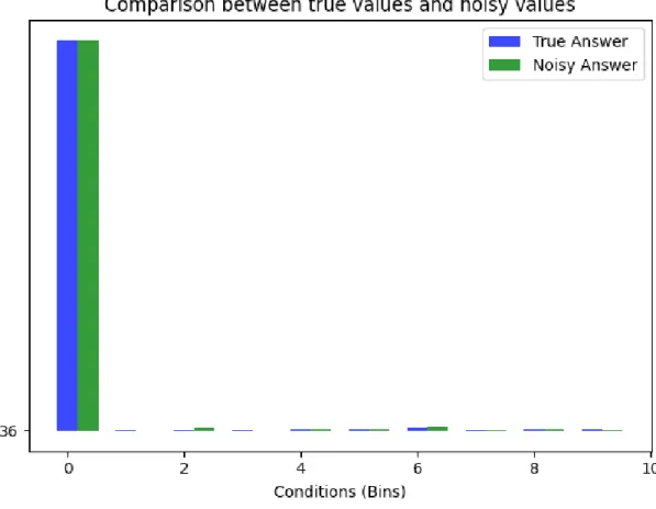
4.2.1 True values, Noisy values and Error metrics for WCQ query for single table database. . . 43

4.2.2 Bar graph for WCQ query for single table database. . . 44

4.2.3 True values, Noisy values and Error metrics for WCQ query for multi-ple table database. . . 44

4.2.4 Bar graph for WCQ query for multiple table database. . . 45

4.2.5 True values, Noisy values and Error metrics for ICQ query for single table database. . . 45

4.2.6 Bar graph for ICQ query for single table database. . . 46

4.2.7 True values, Noisy values and Error metrics for ICQ query for multiple table database. . . 46

4.2.8 Bar graph for ICQ query for multiple table database. . . 47

4.2.9 True values, Noisy values and Error metrics for TCQ query for single table database. . . 47

4.2.10Bar graph for TCQ query for single table database. . . 48

4.2.11True values, Noisy values and Error metrics for TCQ query for multiple table database. . . 48

Introduction

With the recent advances in data analytics and machine learning, organizations are becoming increasingly interested in utilizing these techniques to generate insights from the data they have. But the biggest hurdle, especially for those organizations that collect private information, is that it becomes challenging to share their data with data analysts without compromising the data’s privacy. Moreover, the released data, when matched with the previous releases or the data released from other orga-nizations, can reveal sensitive data about the participants of the data-set. There are a couple of examples that happened in the past, like the Netflix movie recommenda-tion competirecommenda-tion [23] or the re-identificarecommenda-tion of the medical record of the governor of Massachusetts [2]. Both of these incidents happened by matching the data releases of two different organizations. Because of this, various methods exist like anonymizing the data, data encryption, secure multi-party computation, but none of them are good enough or are not easy to implement on the complex datasets. In 2006, Cynthia Dwork et al. [4] came up with something called differential privacy. It helps to en-sure that data privacy remains intact even after publishing the aggregate information about the data. Differential privacy does this by adding Laplacian noise to the actual result of the query. Since then, differential privacy has gained a lot of popularity and has been implemented by organizations like Google, Uber, and Apple to securely share the private data that they collect from the consumers of their products.

1.1

Differential privacy

Differential privacy is used to share data publicly without risking the confidentiality of the participants of the data. Another way to think about differential privacy is that it uses various mechanisms to add noise to the aggregate information about the statistical database. It is difficult for the adversary to infer private data from the par-ticipants of the dataset. For example, various government agencies use differentially private algorithms to publish public data by maintaining the confidentiality of survey responses. Even companies use differentially private algorithms to collect information about user behavior.

In other words, we can consider an algorithm to be differentially private if anyone seeing it’s output cannot identify if some record belongs to a particular individual. It also does not adequately protect from identification and reidentification attacks; it resists such attacks. [7]

Differential privacy has its origins from cryptography, and a lot of its language is from cryptography.

Data Analysts often work on data released by organizations like Healthcare, Bank-ing, and Consumer to help them make informed decisions and gather insights to better their processes and also to serve their customers better. But it does not come without putting private data on the risk of being used in a harmful way. Someone can eas-ily use someone’s banking data for money laundering. They can identify someone’s private health data and make it public as it happened in the case of the governor of Massachusetts. This is where differential privacy[8] comes very handy to stop these kinds of attacks and financial risks for these organizations and allow them to publicly release their data for Data analysts to review and help them make decisions. This means that even if we modify a single record, it does not significantly change the result than the result that we get without making that change. For example, suppose if we have only one person with a particular characteristic present in the dataset. If we release this data publicly without differential privacy, then the adversary can easily run queries to check how many people are present who do not have that

char-acteristic and can easily get the private data of that person. But if we release the data using a differentially private algorithm, then it will be difficult for adversary to find someone’s private data even if the adversary has prior knowledge of that record. We call the change of one record in two similar datasets to be bounded with , where is privacy-loss budget.

1.2

Why do we need Differential Privacy?

Government organizations have long been collecting information about individuals or establishments and sharing that data for multiple reasons. But it is not possible to share all of the data as it is, even though they share only the statistics about the data because it can lead to private data. For example, in 1790, the United States conducted a census where they collected information about people living in the United States and released statistics related to sex, age, race. Not only the U.S. but every country conducts these types of data collections to get a better understanding of their population and then publish the statistics about this data. This data is then used later on for helping governments to make policies and to decide where to project their funding, the marginalized areas of the society, and similar decisions. They share this data with private organizations as well to help them with their choices. For example, banks use this data to decide the risk levels of a particular loan and real estate companies use it to determine if it is safe to sell houses to someone. For public data distribution, government agencies have long been using data suppression to help preserve data that can be compromised. For example, a record with information about only one person or one company is removed to maintain confidentiality.

Since the 1950s and 1960s, there has been rapid adoption of electronic information systems by statistical agencies. This made the public distribution of statistical data more difficult even after data suppression. For example, there is a business whose sales numbers have been suppressed because of the risk of privacy disclosure, but if the same numbers were used in total sales of a region, then the adversary can easily estimate the actual numbers by subtracting the other sales from the total sales of that

region. Not only this, but there are various combinations of additions and subtractions that might put the privacy of the participants of the dataset. The combinations like this increase exponentially with the increasing number of publicly shared data, and this problem become more prominent when we add an interactive query system into the picture.

1.3

Randomized Response (Plausible Deniability)

To understand differential privacy, an understanding of a randomized response is fundamental. Some readers struggle with understanding differential privacy without knowing a randomized response or plausible deniability. The randomized response is a survey technique used by surveyors to collect sensitive information from the sur-vey takers while maintaining the confidentiality of their responses. In a randomized response mechanism, n individuals answer a survey with one binary question. The truthful answer for individual iisxi ∈ {0,1}. The surveyor gives every individual an

unbiased coin and tells them to answer ”Yes” or one if it comes tail and to answer truthfully in case of heads. In this way, every individual gets the opportunity to po-tentially lie and hence the plausible deniability, which helps in keeping their responses confidential. And at the same time, as we know that there is a half-half probability of tails and heads, we can easily double the percent of ”Yes” or ”No” responses to get the actual picture. For example, if we ask the survey takers if they are taking a particular drug, if the number of survey takers who are taking the drug is 20%, then the actual percent of survey takers who are taking that drug would be the double of the number that we got from the survey that is 40%.

1.4

-differential privacy

Cynthia Dwork et al.[4] introduced the concept of -differential privacy in 2006. The main idea behind this work was that if some individuals did not take a survey, it would not be possible to compromise that individual’s privacy. Hence, in differential

privacy, the focus is on giving each individual the amount of privacy that would result from not taking the survey. That is, the transformations and the aggregate function results should not change significantly by removing one individual’s responses to the survey.

Differential Privacy mechanisms achieve this, adding noise before returning the aggregate or other transformation functions run on the survey responses. Now, as we increase the number of survey takers, we would have to add less noise and vice versa.

1.4.1

Definition of

-differential privacy

Definition 1 (-Differential Privacy) A randomized mechanism M : D→ O satisfies

-differential privacy if

P r[M(D)O]≤eP r[M(D0)O] (1) for any set of outputs O ⊆ O, and any pair of neighboring databases D,D0 such that

|D\D0∪D0\D| = 1. [9]

Smaller the value of, more is the privacy, but the amount of noise added will also be high. So, the differential privacy mechanisms try to find a middle ground with the smallest possible value of . The noise added is also not too high, and the result is usable to the data analyst.

1.5

Laplace mechanism

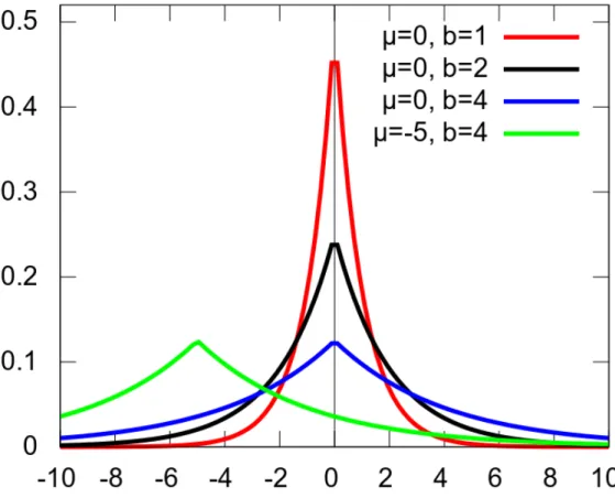
The Laplace mechanism adds noise from the Laplace distribution, as shown in Figure 1.5.1. In Laplace distribution, the mean is zero, and the standard deviation is√2λ.

Let us see an example to understand why adding noise from Laplace distribution gives us differentially private results. Let us say we have a dataset that contains mental health data, and there is an attacker named Eve, and she wants to see if her target, Bob, is receiving counseling for alcoholism or not. If the query’s result

Fig. 1.5.1: Laplace Distribution

comes up as 48, then Eve will know that Bob is receiving counseling for alcoholism. Otherwise, if the query’s result is 47, then he is not receiving counseling for alcoholism. Now since we are using the Laplace mechanism, it does not matter what the actual result of the query is, the mechanism is going to add noise from Laplace Distribution. So, it is going to return results somewhat near 47 or 48. It may be 49, 46, or maybe even smaller like 44 or higher like 51. So, it is practically impossible for Eve to be very sure whether the true answer was 47 or 48. In other words, her belief about Bob (whether he is in counseling for alcoholism or not) will not meaningfully change after running the query.

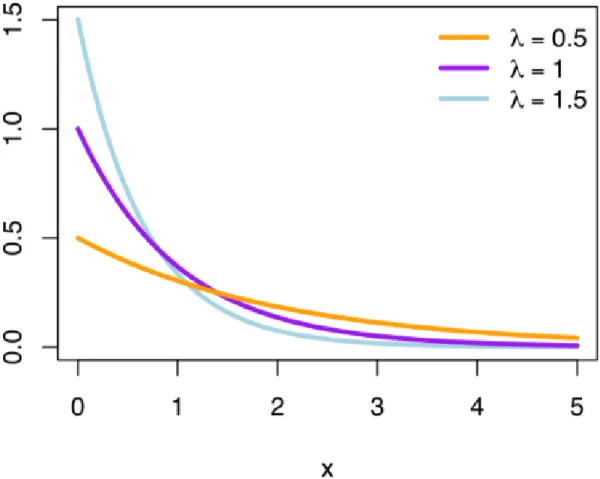
Fig. 1.6.1: Exponential Distribution

1.6

Exponential mechanism

It is used for functions that do not return a real number. For example, ”What is the most common nationality in a particular room?” Chinese/Indian/Canadian.. This is also used when a small change in the output leads to invalid outputs.

Exponential mechanism is most general approach which captures all possible dif-ferential privacy mechanisms. In fact, Laplace distribution is a symmetric exponential distribution (Figure 1.6.1).

1.7

Objectives and Contribution

Even though lot of work has been done on differential privacy and it seems very promising, but it still poses a lot of burden on data analysts to understand differential privacy and manage privacy budgets accordingly. Moreover, this also does not give any accuracy guarantees to the data analyst. Keeping this in mind, Chang Ge et al.[9] introduced a novel system called APEx in May 2019, which allows data analysts to run a sequence of queries keeping privacy and accuracy in place. APEx translates queries and accuracy bounds to differentially private algorithms with the least privacy loss. By doing this, the data analyst gets the answers to its queries, keeping accuracy bounds in place, and the privacy budget set by the data owner is also not exceeded. This experiment has a lot of potential for improvements; for example, Change Ge et al.[9] did these experiments only on a relational database with only one table. In this work, I extended this to multiple tables given that in the real world, data spread across numerous related tables.

The following contributions were made in this research :

• The main idea behind this work is to extend and evaluate APEx which currently is based on Single table to multiple table database schema as mentioned by the author of the paper[9] himself :

“We consider the sensitive dataset in the form of a single-table relational schema R(A1,A2, . . . ,Ad ), where attr(R) denotes the set of attributes of R. Each attribute Ai has a domain dom(Ai). The full domain of R is dom(R) = dom(A1)x....x dom(Ad ), containing all possible tuples conforming to R. An instance D of relation R is a multiset whose elements are tuples in dom(R). We let the domain of the instances be D. Extending our algorithms to schemas with multiple tables is an interesting avenue for future work.”

• I have used a multiple table schema “Employees”.

• Then I made code changes in APEx repository so that when the user run a WCQ, ICQ or TCQ query, instead of the data coming from only one table

(which was the case in existing work), the data is coming from multiple tables. • Then I did a comparison study when we run the APEx on single table vs.

Multiple table.

• I incorporated other error measures such as MSE (Mean Square Error), Mean Absolute Error (MAE), Mean Absolute Percentage Error.

Related Work

Data exploration is becoming more and more important as more and more data is generated by the organizations. Since the last decade, there has been a massive explo-sion in digital data, also referred to as Big Data. With this vast availability of data, it gives an excellent opportunity to data analysts to better improve their analysis. Datasets consist of both public and private data, and exploring them involves a lot of operations such as summarization, building histograms, and building models for ma-chine learning. Incorporating private data into data analytics provides a high value to the data analytics project. Still, often data owners hesitate to give access to the private data because of the risk of data leakage. It could be because of a lot of reasons such as, they do not trust the data analysts or the risk of data leakage is higher than the benefit from the data analytics. For example, Facebook recently announced that they would allow the academic study of their data to find the correlation between social media and politics, specifically in elections. But their main concern was the privacy of their data [15].

Differential privacy is something that has come up as a solution to the problem of public data distribution or at least to an outside organization. It is because of various reasons such as

• It provides a sense of data privacy even when prior knowledge about the data is available.

• It is mathematically proven method to preserve privacy of individual records when aggregate data results are released.

• Even though there is still some information leakage, it can help to keep the leakage bounded.

That is why differential privacy is gaining popularity among data owners such as the US Census Bureau [12, 20, 31], Google [10], Apple [11], and Uber [13].

2.1

Privacy Integrated Queries (PINQ)

Frank McSherry first proposed Privacy INtegrated Queries (PINQ) in his paper[21]. It is a common platform used for differentially private data analysis. It provides an in-terface to data that looks very much like LINQ (C#’s ”language-integrated queries”). All-access through the interface to the data is guaranteed to be differentially private. In PINQ interface, data analysts who are non-privacy experts, write arbitrary LINQ code against datasets in C#.

v a r d a t a = new PINQueryable<SearchRecord>( . . . ) ;

v a r u s e r s = from r e c o r d i n d a t a

where r e c o r d . Query == argv[ 0 ] groupby r e c o r d . IPAddress ;

C o n s o l e . W r i t e L i n e (argv[ 0 ] + ‘ : ‘ + u s e r s . Count ( 0 . 1 ) ) ;

Rather than providing direct access to the underlying data, each private data source is wrapped in a PINQueryable object. This PINQueryableobject is then responsible for mediating accesses to the underlying data, remembering how much privacy budget is left, deducting from the budget whenever an aggregation operator is applied to this PINQueryable object and denying access once the given privacy budget is exhausted.

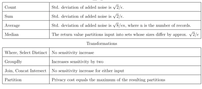
Table 2.1.1 summarizes the main data operations supported by PINQ and their privacy implications. There are two types of operations: aggregations and transfor-mations. Aggregations return the aggregate value after adding noise per differential

Aggregations Count Std. deviation of added noise is√2/. Sum Std. deviation of added noise is√2/.

Average Std. deviation of added noise is√8/n, where n is the number of records. Median The return value partitions input into sets whose sizes differ by approx. √2/

Transformations Where, Select Distinct No sensitivity increase

GroupBy Increases sensitivity by two

Join, Concat Intersect No sensitivity increase for either input

Partition Privacy cost equals the maximum of the resulting partitions

Table 2.1.1: Main data operations in PINQ.

privacy. Transformations return a new PINQueryable object that can be further operated upon. They can amplify the sensitivity of subsequent queries, so that ag-gregations run with one value of may deplete many multiples of from the privacy budget. PINQ ensures that any amplification is properly accounted for. Importantly, the logic within a transformation can act arbitrarily on the sensitive records.

The semantics of the transformations are similar to SQL, with two significant exceptions. First, the join operation in PINQ is not a standard equijoin, in which one record can match an unbounded number of other documents. Instead, records in both dataset are grouped by the key they are being joined on so that the Join results in a list of pairs of groups. This restricts each pair to have a limited impact on aggregates (that of a single record) despite being arbitrarily large, but it does enable differential privacy guarantees which would not otherwise exist.

A second difference is a Partition operation that can split a single protected dataset into multiple protected datasets, using an arbitrary key selection function. This operation is essential because the privacy cost to the source data set is the maximum of the costs to the multiple parts, rather than their sum. We can, for example, partition packets based on the destination port, and conduct independent analyses on each piece while costing only the maximum.

what the analysis aims to output but also on how it is expressed. PINQ is essentially a programming language, and the space of analyses that can be expressed is limited mainly by the analyst’s creativity.

An Example

Suppose we want to count distinct hosts that send more than 1024 bytes to port 80. This computation, which involves grouping packets by source and restricting the result based on what we see in each group, can be expressed as:

p a c k e t s = new PINQueryable<Packet>( t r a c e , e p s i l o n ) ; p a c k e t s . Where ( pkt => pkt . d s t P o r t = 8 0 )

. GroupBy ( pkt => pkt . s r c I P )

. Where ( grp => grp . Sum( pkt => pkt . l e n ) > 1 0 2 4 ) . Count ( e p s i l o n q u e r y ) ;

The Packet type contains fields that we might expect, including sensitive areas such as IP addresses and payloads. The raw data lies in the trace. The total pri-vacy budget for the trace is epsilon, and the amount to be spent on this query is epsilon query. The analyst can run multiple queries on the data as long as the to-tal privacy cost is less than epsilon. The expressions of the form x =⇒ f(x) are anonymous functions that apply f to x.

2.2

Weighted Privacy Integrated

Queries (wPINQ)

Like Privacy Integrated Queries (PINQ) [21], Weighted PINQ is a declarative gramming language over datasets that guarantees differential privacy for every pro-gram written in the language. I refer the reader to [21] for details on the design phi-losophy behind these languages, and to [27] for full technical information on Weighted PINQ’s operators. Here I only provide a short overview of how queries are written in Weighted PINQ.

2.2.1

Overview

Weighted PINQ can apply two types of operators to a (secret) dataset: transfor-mations, and noisy aggregations. Transformation operators such as Select, Where, GroupBy, SelectMany, Join, etc. transform a weighted secret dataset and then au-tomatically rescale the resulting record weights to maintain privacy on the total dis-closure of the records. After doing these transformation operations, the datasets remain secret. Before releasing the final results to the user, the results must be fed to noisy aggregation operators such as NoisyCount. NoisyCount operator aggregates the weighted confidential records, adds Laplace noise and then only exposes the fi-nal results to the end-user. After performing each transformation operator, record weights are scaled-down in such a manner that guarantees differential privacy after noisy aggregation.

2.2.2

Weighted PINQ vs. PINQ

Weighted PINQ is very similar to PINQ in terms of operators. Still, because it operates on weighted records with arbitrary weights (instead of integral weights), it differs from PINQ in few crucial ways:

First, transformations in PINQ that required either scaling up the noise or the privacy parameter , now scale down the weights associated with records. For ex-ample, the operator ‘SelectMany‘, which produces many records (e.g., k (number of records)), scales down each record with a factor of k. The operator GroupBy collects records, results in a group with weight divided by 2, and the operator Join which produces the cross-product of records, with weights rescaled.

The other main difference is a transformation operator to manipulate weights, Shave, which takes a sequence of weights wi and then transforms each record x with

weight w into the set of records (0, x),(1, x), ... with weights w0, w1, ..., for as many

terms as P

iwi ≤ w. Select is the functional inverse of Shave, which can transform

eachwi-weighted indexed pair from (i, x) toxwhose weight re-accumulates to

P

iwi =

Finaly, Weighted PINQ’s operator NoisyCount now rather than returning a single noisy count, returns a dictionary from records to noised weights. This means that if one looks up the value of a record which is not in the input, a weight of zero is introduced, and then the noise is added. This is in some sense generalization of PINQ’s NoisyCount to weights and multi-output “histogram queries” [5]. To repro-duce PINQ’s NoisyCount we can first map all records to some known value, e.g., true.

2.2.3

Writing “good” queries

Now, this brings us to the conclusion that when a query is expressed using Weighted PINQ operators (i.e., transformations, followed by aggregations), it is sufficient to say that it provides differential privacy. So, what remains after this is to write a “good” Weighted PINQ query. There are two main things that we have to look into while writing a good quality query: its computational complexity and its accuracy. Writing “good” queries requires inventiveness. For example, the below query is an example of a query that provides high efficiency and performance, keeping the loss of privacy to the minimum. It is essential to note on the important thing here that it can be more challenging to write “good” queries that directly measure properties with high sensitivity [5] (e.g., graph diameter). One way to get around this is to combine indirect measurements with probabilistic inference.

v a r deqCCDF = e d g e s . S e l e c t ( e d g e => e d g e . s r c ) . Shave ( 1 . 0 )

. S e l e c t ( ( i n d e x , srcname ) => i n d e x ) ; v a r c c d f C o u n t s = degCCDF . NoisyCount ( e p s i l o n ) ;

2.3

Differential Privacy for SQL Queries (FLEX)

Noah Johnson et al. [13] introduced Elastic Sensitivity for efficiently calculating query sensitivity without requiring changes to the database management system (DBMS)

Fig. 2.3.1: Architecture of FLEX from [13].

in their paper . The techniques described in the article provide an en-to-end system to facilitate differential privacy for real-world SQL queries.

Before FLEX[13], the existing differential privacy mechanisms at that time did not support the wide variety of features and databases which were used in real-world SQL-based analytics systems. FLEX [13] was a system built at Berkeley to enforce differential privacy for SQL queries using elastic sensitivity. Noah Johnson et al. [13] discusses how FLEX is compatible with all existing databases, manages to enforce differential privacy requirements for all SQL queries and has a negligible performance overhead.

FLEX relies on the concept of elastic sensitivity. Elastic sensitivity is a novel ap-proach for calculating an upper bound on a query’s local sensitivity. Global sensitivity does not have adequate generalized support for joins in queries. Elastic sensitivity benefits from local sensitivity for queries with general equijoins. Its approach models the impact of each join that is represented in the query, using precomputed metrics about the frequency of join keys in the actual database. This allows the method to compute approximate local sensitivity without additional interactions with the database.

Elastic sensitivity supports several different aggregation functions such as sum, average, max and min. Also, calculations for elastic sensitivity can optimize for

non-sensitive information in the database, helping create tighter bounds for the ap-proximation of local sensitivity. Due to its low computational cost, its adaptability to almost all existing database formats, the current implementation in the form of FLEX, and the general privacy guarantees provided by it, elastic sensitivity can be seen to be a very effective method for ensuring differential privacy.

2.4

KTELO : A Framework for Defining

Differentially-Private Computations

The paper KTELO [32] by Zhang et al. talks about a framework to carry out privacy-preserving computations over data. We can say it is derived from frameworks such as PINQ [12], which extends the (non-private) LINQ framework, and Weighted PINQ.KTELO [32] extends these by providing a different selection of operators with higher level of abstraction to the user who does not have knowledge about differential privacy.

2.5

APEx (Accuracy-Aware Differentially Private

Data Exploration)

APEx [9] built by Change et al. helps to bridge the gap between complex differential privacy mechanisms and Data Owner/ Data Analysts. Even though we know that by adding Laplace noise to the data exploration queries provides differentially private results, the amount of noise or the Laplace distribution from which the noise is calcu-lated depends on the data. So, APEx is built to help Data Owner/Data Analyst as shown in Figure 2.5.1 to focus on their work by just providing the privacy budget and accuracy bounds and leaving the rest to the APEx to figure out which mechanism and input factors to the mechanism would be best. APEx mainly covers three types of data exploration queries:

Fig. 2.5.1: Workflow of APEx [9].

2. Iceberg Counting Query (ICQ) 3. Top-k Counting Query (TCQ)

As we have discussed earlier, there exist general-purpose private query answering systems; they are not interactive and mainly lack two main aspects. Firstly, these systems expect the data analysts to have in-depth knowledge of differential privacy and differentially private algorithms, which most often do not. For example, PINQ [12] and wPINQ [28] allow users to write differentially private programs and ensure that every program expressed satisfies differential privacy. PINQ provides an SQL-like interface to the data analysts. Similarly, using a few simple operators (including a non-uniformly scaling Join operator), wPINQ can reproduce (and improve) several recent results on graph analysis and introduce new generalizations (e.g., counting triangles with given degrees). However, to achieve high efficacy of the system, the analyst has to be familiar with the intricate literature of data privacy to understand how the differentially private algorithms add noise and know if the desired accuracy level can be achieved in the first place. ktelo [32] tried to mitigate this problem by giving access to high-level operators to the data analyst that can be composed to create accurate differentially private programs to answer counting queries. However, the analyst is still expected to know how to distribute privacy budgets across different operators optimally. Similarly, FLEX [13] provides users with an interface to answer

one SQL query under differential privacy but has the same issue of distributing privacy budget when tested across a sequence of queries. Secondly, and somewhat ironically, these systems do not provide any assurance to the data analyst on the quality they care about, namely the accuracy of query answers. Most of these systems depend on the privacy level () as input to figure out the most feasible differentially private algorithm without considering the accuracy of the result of the query.

This was the primary purpose behind APEx, to design a system that does not only allow data analysts to explore a sensitive dataset D held by a data owner by running a sequence of queries with high accuracy but also keeping the query results under the privacy budget set by the data owner. The system mainly focused on these two main functions: (1) as the data is sensitive, the data owner is assured that any information leakage is bounded under the privacy budget of any individual record in dataset D; and (2) also as the addition of noise affects the accuracy of the query result, it is still under the accuracy bounds set by the data analyst. The main features of APEx involved:

• To support declaratively specified aggregate queries that capture a wide variety of data exploration tasks.

• To allow analysts to specify accuracy bounds on queries.

• To translate an analyst’s query into a differentially private mechanism with minimal privacy lossso that it can answer the query set, keeping the accuracy bounds checked.

• To prove that for any interactively specified sequence of queries, the analyst’s view of the entire data exploration process satisfiesB-differential privacy, where B is an owner specified privacy budget.

Ligett et al. [19] also worked on similar work as APEx, which also considered ac-curacy constraints specified by data analysts. While their work focused on finding the smallest privacy cost for a given differentially private mechanism and accuracy bound, APEx focus was on a more general problem: for a given query, find a mechanism and

a minimal privacy cost to achieve the given accuracy bound. Moreover, APEx was tested on a single table MYSQL database. As we know that in real-life, data spread across multiple related database tables. In this work, APEx is extended/tested on multiple-table database. This helped to get a better picture of the applicability of this niche concept on a relational multi-table database.

2.6

Internal structure of APEx

This section gives an outline of how APEx translates queries set by the data analyst along with the accuracy budget into differentially private mechanisms, and how it ensures that the privacy budget B specified by the data owner is also not violated. The main functionality of the extended APEx remains the same as the actual functionality of APEx. The only main difference is that the result of the queries is from multiple database tables instead of only one table. APEx consists of two parts:

1. Accuracy Translator 2. Privacy Analyzer

2.6.1

Accuracy Translator

This section covers the accuracy-to-privacy translation mechanisms supported by APEx and the corresponding run and translate functions. In the original APEx paper, the author has discussed two types of transformations for all three types of queries: (1) Baseline Transformation and (2) Special Transformation. In this work, I have focussed my study on Baseline Transformation only, which is discussed in more detail later.

Given an analyst’s query (q, α, β), APEx first uses the accuracy translator to choose a mechanism M that can (1) answer q under the specified accuracy bounds set by the data analyst, and also with (2) minimal privacy loss and under the privacy budget set by the data owner. To achieve this, APEx supports a set of differentially private mechanisms that can be used to answer each query type (WCQ, ICQ, TCQ).

Multiple mechanisms are supported for each query type as different mechanisms result in the least privacy loss depending on the query and the dataset.

For each query of the user, APEx has to make sure that the answer is between the accuracy and the privacy bounds. To achieve this, it contains various differential privacy mechanisms, and each of these mechanisms is most effective depending on the query and the dataset. Thus, each mechanism M has two functions:

1. M.TRANSLATE 2. M.RUN

When a mechanism M is executed, M.TRANSLATE is responsible for translating a query and accuracy requirement into lower and upper bound (l, u) on the privacy loss. After that, M.RUN runs the differentially private algorithm and returns an approximate answer ω for the query. The answer ω is guaranteed to satisfy the specified accuracy requirement. Moreover, M also fulfills u _{differential privacy.}

Algorithm 2.6.1 APEx Overview [9]

Require: Dataset D, privacy budget B 1: Initialize privacy lossB0 ⇐0, indexi⇐1

2: repeat

3: Receive (qi, αi, βi) from analyst

4: M ⇐ mechanisms applicable to q‘ is type

5: M∗ ⇐ {M ∈ M|M.TRANSLATE(qi, αi, βi).u ≤B−Bi−1}

6: if M∗ 6=∅ then

7: //P essimistic M ode

8: Mi ⇐argminM∈M∗M.T RAN SLAT E(q_i, α_i, β_i).u

9: //Optimistic M ode

10: Mi ⇐argminM∈M∗M.T RAN SLAT E(q_i, α_i, β_i).l

11: (ωi, i) ⇐ Mi.RUN(qi, αi, βi, D)

12: Bi ⇐Bi−1+i, i++ return ωi

13: else

14: Bi =Bi−1, i++ return ’Query Denied’

15: end if

16: until No more queries sent by local exploration

As described in Algorithm 2.6.1, APEx first identifies the mechanisms M that are applicable for the type of the query qi (Line 4). Next, it runs M.translate to get

conservative estimates on privacy loss u _{for all these mechanisms (Line 5). APEx}

picks one of the mechanisms M from those that can be safely run using the remaining privacy budget, executes M.run, and returns the output to the analyst. As we will see, there exist mechanisms where the privacy loss can vary based on the data in a range between [l_, u_{], and the actual privacy loss is unknown before running the mechanism.}

In such cases, APEx can choose to be pessimistic and pick the mechanism with the least u (Line 8), or choose to be optimistic and pick the mechanism with the least l (Line 10).

2.6.1.1 Matrix Transform

The workload in (WCQ,ICQ,TCQ) queries is represented in a matrix form, like the prior work for WCQ [17, 18, 20]. A workload can be transformed in many possible ways. Given a query with L predicates, the number of domain partitions can be as large as 2L _{. In this work, the following transformation is considered to reduce}

complexity. Given a workload counting query qW with the set of predicates W =

{φ1, ..., φL}, the full domain of the relation dom(R) is partitioned based on W to

form the new discretized domain domW(R) such that any predicate φi ∈ W can be

expressed as a union of partitions in the new domain domW(R) and the number of

partitions are minimized. For example, givenW ={Age >50∧State=AL, ..., Age > 50∧ State = W Y}, one possible partition is domW(R) = {Age > 50∧ State =

AL, ..., Age >50∧State=W Y, Age ≤50}.

Let x represents the histogram of the table D over domW(R). The set of the

corresponding counting queries {cφ1, ..., cφL} for qW can be represented by a matrix

W = [w1, ..., wL]T of size L× |domW(R)|. Hence, we can say that the answer to each

counting query is simply cφi(D) = wi.x, and the answer to the workload counting

query is simply Wx. This transformation denoted by W ← T(W), x ← TW(D) is

used throughout later. Prior work such as [17, 18, 20] were based on to bound the total expected error on single query. APEx differs from them by bounding the maximum error per query with high probability which is more instinctive in the process of data exploration.

2.6.1.2 Baseline Translation

For the baseline translation for all three query types in APEx, the Laplace mecha-nism is used [6, 8]. Laplace mechamecha-nism is widely used and accepted as a standard differentially private mechanism.

Definition 2 (Laplace Mechanism (Vector Form)[6, 8]). Given an L× |domW(R)|

query matrix W, the randomized algorithm LM that outputs the following vector is

-differentially private: LM(W, x) =W x+Lap(bw)L where bw =

||W||1

, and Lap(b) L

denote a vector of L independent samples ηi from a Laplace distribution with mean 0

and variance 2b2_{, i.e., P r[η}

i =z]∝e−z/b for i=1,...,L. [9]

The sensitivity of queries set defined by the workload W [17, 18] is equal to the constant ||W1||. This constant calculates the maximum difference in the answers to

the queries in W when these queries are run on any two databases that differ only by a single record. Mathematically, it is the maximum of the L1 norm of a column of W.

Algorithm 2.6.2 presents the run and translate of Laplace mechanism for all three query types. In this algorithm we can see that first the queryqW and the data D are

converted into matrix representation W and x, respectively. The translate generates a lower and upper bound (l, u) for each query type with a given accuracy require-ment and since Laplace mchanism is data independent, these two bounds are same. However, these bounds vary among query types. The run takes the privacy bud-get computed by TRANSLATE(q, α, β) (Line 3) and adds the corresponding Laplace noise [ ˜x1, ...,x˜L] to the true workload counts Wx. In case of when q is a Workload

Counting Query (WCQ), the noisy counts are returned directly at the end of running the Laplace mechanism. When q is an Iceberg Counting Query (ICQ), the bin ids (the predicates) that have noisy counts ≥ c are returned. And, when q is a Top-k Counting Query (TCQ), the bin ids (the predicates) that have the largest k noisy counts are returned. Along with the noisy output, the privacy budget consumed by this mechanism is also returned. The following theorem provide a summarization of the properties of the two functions run and translate.

Algorithm 2.6.2 Laplace Mechanism (LM) (q, α, β, D) [9] 1: Initialize W ← T(W ={φ1,· · ·, φL}), x← TW(D), α, β

2: function RUN(q, α, β, D)

3: ←T RAN SLAT E(qW, α, β, D).u

4: [˜x1,· · · ,x˜L]←W x+Lap(b)L, whereb =||W||1/

5: if q.type==WCQ (i.e.,qW)then

return ([˜x1,· · · ,x˜L],)

6: else if q.type==ICQ (i.e., qW,>c) then

return (φi ∈W|x˜i > c,)

7: else if q.type==TCQ (i.e., qW,k) then

return (argmaxk

φ1,···,φLx˜i,)

8: end if

9: end function

10: function TRANSLATE(q,α,β)

11: if q.type==WCQ (i.e.,qW)then

return (u ₌ ||W||1ln 1/(1−(1−β)1/L))

α , l₌u₎

12: else if q.type==ICQ (i.e., qW,>c) then

return (u = ||W||1(ln 1/(1−(1−β)1/L))−ln 2)

α ,

l ₌u₎

13: else if q.type==TCQ (i.e., qW,k) then

return (u ₌ ||W||12(ln (L/(2β)))

α ,

l₌u₎

14: end if

Theorem 1 Given a query q where q.type ∈ {W CQ, ICQ, T CQ}, Laplace mecha-nism (Algorithm 2.6.2) denoted by M can achieve(α, β)−q.typeaccuracy by executing the function RU N(q, α, β, D) for any D∈ D, and satisfy differential privacy with a minimal cost of TRANSLATE(q, α, β).u_{. [9]}

The accuracy and privacy proof is mainly based on the noise property of Laplace mechanism.

2.6.2

Privacy Analyzer

Given a sequence of queries (M1, ..., Mi) that has already been executed by the privacy

engine and that satisfy an overall Bi−1-differential privacy. If a new query (qi, αi, βi)

is run, APEx first identifies a set of mechanisms M∗ that all will have a worst-case privacy loss smaller than B −Bi−1 (Line 5 in Algorithm 2.6.1). That is, running

any mechanism in M∗ will not result in exceeding the privacy budget in the worst case. If M∗ = ∅, then APEx returns ‘Query Denied’ to the analyst (Line 16 in Algorithm 2.6.1). Otherwise, APEx runs one of the mechanisms Mi from M∗ by

executing Mi.RUN() and the output ωi will be returned to the analyst. APEx then

increments Bi−1 by the actual privacy loss i rather than the upper bound u (Line

12 in Algorithm 2.6.1).

The privacy analyzer ensures that every sequence of queries answered by APEx results in aB-differentially private execution, where B is the privacy budget specified by the data owner. The formal proof of privacy primarily follows from the well-known composition theorems. According to sequential composition, the privacy loss of a set of differentially private mechanisms (that use independent random coins) is the sum of the privacy losses of each of these mechanisms. Moreover, postprocessing the outputs of a differentially private algorithm does not degrade privacy.

The main critical part of the privacy proof (described in Section 3.2.2.1) arises since (1) the parameter for a mechanism is chosen based on the analyst’s query and accuracy requirement, which in turn are adaptively chosen by the analyst based on previous queries and answers, and (2) some mechanisms may have an actual privacy

loss dependent on the data. APEx accounts for privacy based on the actual privacy loss (and not the worst case privacy loss) (see Line 12, Algorithm 2.6.1).

2.6.2.1 Overall Privacy Guarantee

Privacy guarantee means that given any sequence of interactions between the data analyst and APEx, APEx satisfies B-differential privacy, where B is the privacy budget specified by the data owner. To state this guarantee formally, we first need to understand a record of the interaction between APEx and the data analyst.

We define the transcript of interaction _T as an alternating sequence of queries (with accuracy requirements) set to APEx by the data analyst and answers returned by APEx. _T depicts the analyst’s view of the private database. More formally,

• The transcript _Ti after i interactions is a sequence

[(q1, α1, β1),(ω1, 1),· · · ,(qi, αi, βi),(ωi, i)], where (qi, αi, βi) are queries with

accuracy requirements, and ωi is the answer returned by APEx and i the

actual privacy loss.

• Given _Ti−1, analyst choses the next query (qi+1, αi+1, βi+1) adaptively. APEx

model this using a (possibly randomized) algorithm _C that maps a transcript

Ti−1 to (qi, αi, βi); i.e.,C(Ti−1) = (qi, αi, βi). Note that the analyst’s algorithm

C does not access the private database D.

• Given (qi, αi, βi), APEx select a subset of mechanismsM∗ such that∀M ∈ M∗,

M.TRANSLATE(qi, αi, βi).u ≤ B −Bi. Furthermore, if M∗ is not empty,

APEx choses one mechanism Mi ∈ M∗ deterministically (either based on l or

u) to run. The selection of Mi is deterministic and independent of D.

• If APEx find no mechanism to run (M∗ _{= ∅), then the query is declined by}

APEx. In this case, ωi =⊥ and i = 0.

• If the APEx chosen algorithmMi is LM, WCQ-SM, ICQ-SM or TCQ-LTM,i =

u

i, whereiis the upperbound on the privacy loss returned byMi.TRANSLATE.

• Let P r[_Ti|D] denote the probability that the transcript of interaction is Ti

given input database D. The probability is over the randomness in the ana-lyst’s choices _C and the randomness in the mechanisms M1,· · · , Mi executed

by APEx.

Not all transcripts of interactions are realizable under APEx. Given a privacy budget B, the set of valid transcripts is defined as:

Definition 3 (Valid Transcripts [9]). A transcript of interaction_Ti is a valid APEx

transcript generated by Algorithm 2.6.1 if given a privacy budget B the following conditions hold:

• Bi−1 =Pi

−1

j=1j ≤B, and

• Either ωi =⊥, or Bi−1+ui ≤B.

We are now ready to state the privacy guarantee:

Theorem 2 (APEx PRIVACY GUARANTEE[9]). Given a privacy budget B, and valid APEx transcript _Ti,and any pair of databases D, D0 that differ in one row (i.e.,

|D\D0∪D0\D|= 1), we have:

(1) Bi =

Pi

j=1i ≤B, and

(2) Pr[_Ti|D]≤eBiP r[Ti|D0].

More details regarding APEx can be found in APEx[9] research paper.

2.7

Accuracy Measure

The answers to the exploration queries are typically noisy to ensure Differential Pri-vacy. To allow the data analyst to explore data with bounded error, the queries are extended to incorporate an accuracy requirement. The syntax for accuracy is similar to that in BlinkDB [1]:

BIN D on f(·) WHERE W ={φ1, ..., φL} [HAVINGf(·)>c]

[ORDER BY f(·) LIMIT k] ERROR α;

The accuracy requirement for a WCQ qw is defined as a bound on the maximum

error across queries in the workload W.

Definition 4 ((α, β)− W CQ accuracy [9]) Given a workload counting query qw :

D0 →RL _{, whereW ={φ}

1,· · · ,φL }. LetM :D

0

→RL_{be a mechanism that outputs}

a vector of answers y on D. Then, M satisfies (α, β)−W accuracy, if ∀D∈D0,

P r[||y−qw(D)||∞≥α]≤β, (1)

where ||y−qw(D)||∞ =maxj|y[i]−cφi(D)|.

The output of iceberg counting queries ICQ and top-k counting queries TCQ are not numeric, but a subset of the given workload predicates. Their accuracy measures are different from WCQ, and depend on their corresponding workload counting query qW.

Definition 5 ((α, β)−ICQ accuracy [9]) Given an iceberg counting query qw,>c :

D0 → O , where W = {φ1, · · · ,φL }, and O is a power set of W. Let M :D

0

→O

be a mechanism that outputs a subset ofW. Then, M satisfies (α, β)−ICQaccuracy for qw,>c, if for D,

P r[|{φ∈M(D)|cφ(D)< c−α}|>0]≤β (2)

P r[|{φ ∈(W −M(D))|cφ(D)> c+α}|>0]≤β (3)

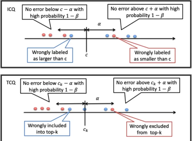
A mechanism for ICQ can make two kinds of errors: label predicates with true counts greater than cas< c (red dots in 2.7.1) and label predicates with true counts less than c as> c (blue dots in 2.7.1).

We say a mechanism satisfies (α, β)−ICQ accuracy if with high probability, all the predicates with true counts greater than c+α are correctly labeled as >c and

all the predicates with true counts less than c−α are correctly labeled as< c . The mechanism may make arbitrary mistakes within the range [c−α, c+α].

Definition 6 ((α, β)−T CQ accuracy [9]) Given a top-k counting queryqw,k:D

0

→ O , where W = {φ1, · · · ,φL }, and O is a power set of W. Let M : D

0

→ O be a mechanism that outputs a subset of W. Then, M satisfies (α, β)−T CQ accuracy if for D ∈ D0,

P r[|{φ∈M(D)|cφ(D)< ck−α}|>0]≤β (4)

P r[|{φ∈(Φ−M(D))|cφ(D)> ck+α}|>0]≤β (5)

where ck is the kth largest counting value among all the bins, and Φ is the true

top-k bins.

The intuition behind Definition 4 is similar to that of ICQ and is explained in Figure 2.7.1: predicates with count greater than ck+α are included and predicates

with count less than ck−α do not enter the top-k with high probability.

The advantages of the accuracy definitions defined above are that they are intuitive (whenαincreases, noisier answers are expected) and we can design privacy-preserving mechanisms that introduce noise while satisfying these accuracy guarantees. On the other hand, this measure is not equivalent to other bounds on the accuracy like relative error and precision/recall which can be very sensitive to small amounts of noise (when the counts are small, or when lie within a small range). For example, if the counts of all the predicates in ICQ lie outside [c−α, c+α], a mechanism M that perturbs counts within±αand then answers an ICQ will have precision and recall of 1.0 with high probability as it makes no mistakes. However, if all the query answers lie within [c−α, c+α], then the precision and recall of the output of M could be 0.

Methodology used and Extensions

to APEx

In this chapter, the extensions to the APEx are covered in more detail.There are some similarities to the APEx, as this is the extension to the original paper. In this work, it is tested on multiple-table dataset. A dataset with multiple tables is used, which is also discussed in detail later in section 3.1. Then the changes to the queries structure were made, which are more evident in the code used to test the concept. The code is attached in the Appendix.

3.1

Dataset

In this research, I have taken multi-table relational schema R1(A1, A2, ..., Ad),

R2(B1, B2, ..., Bd) where attr(R1) and attr(R2) denotes the set of attributes of

R1

S

R2. Each attributeAihas a domaindom(Ai). The full domain of R isdom(R) =

dom(A1)× · · · ×dom(Ad)×dom(B1)× · · · ×dom(Bd), containing all possible tuples

conforming to R. An instance D of relation R is a multiset whose elements are tuples indom(R). Let us denote the domain of the instances be D.

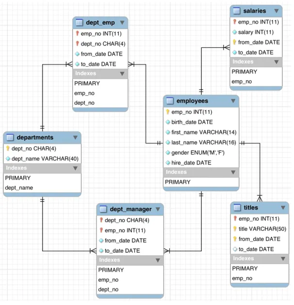
Based on the above multiple-table schema, I found Employee sample database from MYSQL website. Patrick Crews and Giuseppe Maxia [26] developed the Em-ployee sample database and provide a combination of a broad base of data (approxi-mately 160MB), which spread over six separate tables and consists of 4 million records in total. There are about 300,000 employee records with 2.8 million salary entries

Fig. 3.1.1: The Employees Schema

in the database. The diagram 3.1.1 provides an overview of the structure of the Employees sample database.

3.2

Queries and their types

This section describes the different types of queries used in APEx. It is believed that most of the data exploration done by data analysts can be done by writing queries that can be categorized into one of these query types. These queries are commonly referred to as Exploration Queries.

3.2.1

Exploration Queries

There are mainly three types of exploration queries: 1. Workload Counting Query (WCQ)

2. Iceberg Counting Query (ICQ) 3. Top-k Counting Query (TCQ)

3.2.1.1 Workload Counting Query (WCQ)

Workload counting queries cover a large part of Linear Counting queries. They are very similar to SQL SELECT ... GROUP BY queries. Another excellent example of workload counting queries is histogram queries. For example, let’s take a table D with attribute state having domain{AL, AK, . . . , WI, WY} and an attribute Age with domain [ 0,∞). Then, a query to return the number of people with age above 50 for each state can be expressed using WCQ as:

BIN D on COUNT(*) WHERE W = {Age > 50∧ State = AL, ..., Age > 50∧State=W Y};

3.2.1.2 Iceberg Counting Query (ICQ)

The main difference between the iceberg counting query and linear counting query is that the answer to the query is a subset of the predicates in W.

BIN D on COUNT(*) WHERE W = {φ1, ..., φL} HAVING COUNT(*) > c;

An iceberg counting query returns bin identifiers if the aggregated value for that bin is higher than a threshold. For example, a query which returns the states in the US which have a population of at least 5 million can be expressed as:

BIN D on COUNT(∗)

WHERE W = {S t a t e=AL , . . . , S t a t e=WY} HAVING COUNT(∗) > 5 m i l l i o n ;

Note that since the answer to the query is a subset of the predicates in W (i.e. a subset of bin identifiers) but not the aggregate values for these bins, an ICQ is not a linear counting query.

3.2.1.3 Top-k Counting Query (TCQ)

BIN D on COUNT(*) WHERE W ={φ1, ..., φL}

ORDER BY COUNT(*) LIMIT k;

This query firsts sorts all the bins based on a threshold and returns the top k bin identifiers. For example, a query to return the top three US states with the highest population can be written as:

BIN D on COUNT(*) WHERE W = {State=AL, ..., State=W Y} ORDER BY COUNT(*) LIMIT k;

3.3

Code changes on APEx

In order to make APEx compatible with multiple-table queries, there were a couple of changes that were required at the code level. But before that, we need to understand how APEx works at the code level. When we run the program, there are two threads that run simultaneously. First, based on the given values of α,β and the differential privacy mechanism, the estimated cost of differential privacy mechanism and differ-ential privacy mechanism itself is calculated. This can be seen in the following code snippet for mechanisms LM and LM SM.

Listing 3.1: Estimated cost and calculation of mechanism [9]

# e s t i m a t e c o s t u s i n g s e q u e n t i a l c o m p o s i t i o n

def e s t i m a t e l o s s ( s e l f , m) :

# e s t i m a t e t h e c o s t b a s e d on t h e q u e r y t y p e

q = m. q u e r y

i f q . q u e r y t y p e == Type . QueryType .WCQ:

# e s t i m a t e c o s t

e s t c o s t = l m e s t c o s t (m) m. s e t e s t c o s t ( e s t c o s t )

# s e t t h e l a p l a c e b

m. s e t l a p b ( q . g e t s e n s i t i v i t y ( ) / e s t c o s t )

e l i f q . m type == Type . MechanismType . LM SM :

# e s t i m a t e c o s t e s t c o s t = l m s m e s t c o s t (m) m. s e t e s t c o s t ( e s t c o s t ) # s e t t h e l a p l a c e b m. s e t l a p b (m. s t r a t e g y s e n s / e s t c o s t ) return s e l f . t o t a l p r i v a c y c o s t + m. e s t c o s t

As we can see from the above code snippet that first it calculates cost estimation. It is done using this formula.

Listing 3.2: Cost estimation [9]

def l m e s t c o s t (m) :

q = m. q u e r y

e s t c o s t = q . g e t s e n s i t i v i t y ( ) ∗ np . l o g ( 1 . 0 / ( 1 . 0 − ( 1 . 0 − m. b e t a )

∗∗ ( 1 . 0 / len( q . c o n d l i s t ) ) ) ) / m. a l p h a

return e s t c o s t

Sensitivity in the above function is just the sensitivity of the matrix. After calcu-lating the estimated cost of the mechanism, the mechanism itself is calculated as can be seen in Listing 3.1.

Second, the query is converted into a matrix form. This can be seen in the following code snippet.

Listing 3.3: Matrix Representation of query [9]

# c o n s t r u c t t h e m a t r i x r e p r e s e n t a t i o n o f t h e q u e r y

# f o r 1D and 2D h i s t o g r a m , j u s t c o u n t (∗) # g e t a l l t h e c o u n t s f o r e a c h p r e d i c a t e s e l f . d o m a i n h i s t = s e l f . g e t c o n d c o u n t s ( ) # f o r i i n r a n g e ( 0 , l e n ( s e l f . d o m a i n h i s t ) ) : i f s e l f . i n d e x . n a m e in [ ’ qw 1 ’ , ’ qwm 1 ’ , ’ q i 3 ’ , ’ q t 1 ’ , ’ qtm 1 ’ , ’ qw 4 ’ , ’ q i 2 ’ , ’ qim 2 ’ , ’ q t 3 ’ ] : # 1D/2D h i s t o g r a m i s h i s t = True e l s e: i s h i s t = F a l s e i f i s h i s t : # f o r h i s t o g r a m q u e r y c o u n t r o w b y p r e d i c a t e s = sum( s e l f . d o m a i n h i s t ) s e l f . q u e r y m a t r i x = np . z e r o s ( (len( s e l f . c o n d l i s t ) , len( s e l f . d o m a i n h i s t ) ) ) i f i s h i s t : f o r i in range( 0 , len( s e l f . c o n d l i s t ) ) : s e l f . q u e r y m a t r i x [ i ] [ i ] = 1

In order to convert a histogram query to matrix form, first we calculate the domain of the histogram. This is the condition counts. It contains the value corresponding to each condition. Using this and the length of condition list, we get x × y matrix where x is the length of condition list and y is the length of domain of histogram.

These two threads give us the foundation to calculate the final answers to the query. As can be seen from the code snippet of matrix transformation (Listing 3.3) that it calculates the condition counts, which is the primary thing in the type of queries that we are trying to execute. The condition counts are the ones that are shown as bars in a histogram. To calculate these condition counts, the previous version of APEx used to calculate these on a single table, as we can see from this

code snippet.

Listing 3.4: Condition counts for single table schema

c r n t q u e r y = s e l e c t c o u n t (∗) from

+ t a b l e n a m e + where + cond

This is changed to get the condition counts from multiple tables based on the query type as can be seen from the following code snippet.

Listing 3.5: Condition counts for multiple table schema

# p r e p a r e t h e q u e r y t o q u e r y i d s

i f( s e l f . i n d e x . n a m e == ’ qim 2 ’ ) :

c r n t q u e r y = SELECT COUNT(∗) FROM

(SELECT A. emp no , A. ge nd er , B . s a l a r y

FROM e m p l o y e e s . e m p l o y e e s a s A INNER JOIN e m p l o y e e s . s a l a r i e s a s B ON

A. emp no = B . emp no where + cond + ) C

# g e t t h e t o t a l c o u n t from t h e t a b l e

i f( s e l f . i n d e x . n a m e == ’ qim 2 ’ ) :

c r n t q u e r y = SELECT COUNT(∗) FROM (SELECT A. emp no ,

A. ge nd e r , B . s a l a r y FROM e m p l o y e e s . e m p l o y e e s a s

A INNER JOIN e m p l o y e e s . s a l a r i e s a s B ON A. emp no = B . emp no ) C

3.4

Incorporating other measures

Extended APEx is evaluated on various error measures like Mean Square Error (MSE), Mean Absolute Error (MAE) and Mean Absolute Percentage Error. These error measures are widely used in Machine Learning models. The motivation behind using these as error measures for APEx is the existence of an excellent analogy behind a machine learning model and APEx. A machine learning model predicts a value, and we use these measures to see how close that prediction is to the actual value.

Similarly, APEx returns noisy values to the data analyst. These error measures can help us evaluate how close or how accurate these noisy values are to the true val-ues. The more precise these noisy values are, the more beneficial they can be to the data analyst. Since we have used Differentially Private mechanism to calculate these values, the privacy constraint set by the data owner is also kept.

Mean Square Error (MSE): In statistics, Mean Squared Error is widely used measure to determine the performance of an estimator. In simple words, it is the square root of the average of squared differences between the true value and the predicted value. M SE = v u u t 1 n n X j=1 (yj −yˆj)2

Mean Absolute Error (MAE): The main difference in Mean Absolute Error and Mean Square Error is that it measures average magnitude of the errors in a set of noisy answers, without considering their direction. It’s the average over the sample of the absolute differences between the noisy answer and the true answer where all individual differences have equal weight.

M AE = 1 n n X j=1 |yj −yˆj|

Mean Absolute Percentage Error (MAPE): Mean Absolute Percentage Er-ror (MAPE) measures the size of erEr-ror in terms of percentage. It is mostly used to give perspective to how much error is there on scale of 1-100.

M AP E= 1 n n X j=1 |yj−yˆj| ∗100

The error values of these measures are provided in the next chapter. The one important observation to notice is that when we compare the error values from single table queries and multiple table queries, there is not much difference. For example, the error values of WCQ for single table query are 83.4 and 13894.5 for MAE and MSE respectively. Whereas for WCQ for multiple table query, the error values are

87.10, and 9927.95 for MAE and MSE respectively. This re-assures us that APEx can easily be scaled to data which multi-dimensional, multi-table and also with large volume without affecting its error measures.

Experiments and Results

In this research, I have evaluated extended APEx on real-world datasets, out of which two were single-table dataset, and one was multiple-table dataset. The details, along with the entity-relationship diagram about the numerous table dataset, can be found in Chapter 3 (Methodology). Extended APEx was evaluated using a set of benchmark queries to see if :

• APEx can effectively translate queries associated with accuracy bounds into differentially private mechanisms. These mechanisms accurately answer a wide variety of new data exploration queries with moderate to low privacy loss. • The set of query benchmarks show that no single mechanism can dominate

the rest and APEx picks the mechanism with the least privacy loss for all the queries.

4.1

Setup

4.1.1

Datasets

The experiment uses three real-world datasets. The first data set Adult was ex-tracted from the 1994 US Census release [3]. This dataset includes 15 attributes (6 continuous and nine categorical), such as ”capital gain”, ”country”, and a binary ”label” indicating whether an individual earns more than 5000 or not, for a total of 32, 561 individuals. The second dataset, referred to as NYTaxi, includes 9, 710, 124 NYC’s yellow taxi trip records [30]. Each record consists of 17 attributes, such

as categorical attributes (e.g., ”pick-up-location”), and continuous attributes (e.g., ”trip distance”). The third dataset, Employees sample database [25], is taken from the MYSQL website. It was developed by Patrick Crews and Giuseppe Maxia and provides a combination of a large base of data (approximately 160MB) spread over six separate tables and consisting of 4 million records in total.

4.1.2

Query Benchmarks

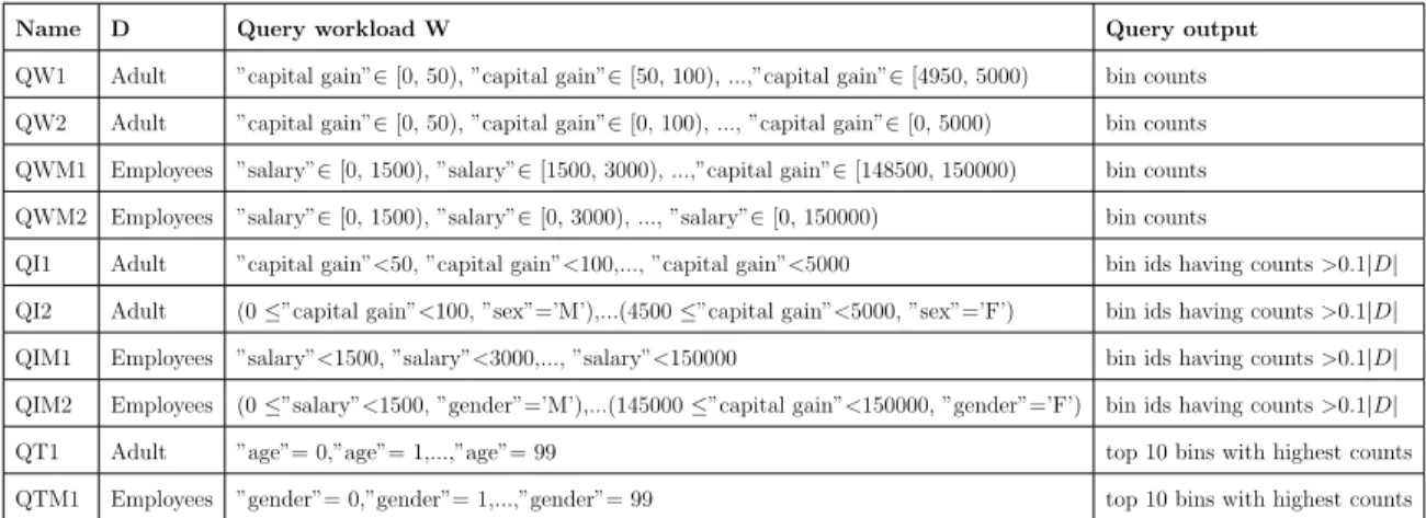
In this research, ten meaningful exploration queries on Adult and Employees datasets, summarized in Table 4.1.1 are tested. These ten queries cover the three types of exploration queries defined in Section 3.3, QW1, QW2, QWM1, QWM2, QI1, QI2, QIM1, QIM2, QT1 and QT2 corresponds to WCQ (Workload Counting Query), ICQ (Iceberg Counting Query) and TCQ (Top-K Counting Query) respectively. Queries with numbers 1 and 2 are for Adult, with numbers M1 and M2 are for Employees dataset. The predicate workload W cover 1D histogram, 1D prefix, 2D histogram and count over multiple dimensions. β = 0.0005 and vary α ∈

{0.02,0.04,0.08,0.16,0.32,0.64}.

4.1.3

Metrics

For each query (q, α, β), APEx outputs (, ω) after running a differentially private mechanism, whereis the actual privacy loss andωis the noisy answer. The empirical error of a WCQ qW (D) is measured as||ω−qw(D)||∞/|D|, the scaled maximum error

of the counts. The empirical errors ofICQqw,>c(D) andT CQqw,k(D) are measured as

||α||∞/|D|, t