Assessing the transferability of machine learning algorithms using cloud computing and earth observation datasets for agricultural land use/cover mapping

(1)

ASSESSING THE TRANSFERABILITY OF MACHINE LEARNING ALGORITHMS

USING CLOUD COMPUTING AND EARTH OBSERVATION DATASETS FOR

AGRICULTURAL LAND USE/COVER MAPPING

Bushra Praveen1_{Sk. Mustak}*,2_{, Pritee Sharm}_a1

1_{Indian Institute of Technology, Indore}

2_{Ashoka Trust for Research in Ecology and Environment, Bangalore, [email protected]/[email protected]} Commission WG III/10

KEY WORDS: Cloud Computing, transferability, Kernel optimization, land use/ land cover; earth observation

ABSTRACT:

Mapping of agricultural land use/cover was initiated since the past several decades for land use planning, change detection analysis, crop yield monitoring etc. using earth observation datasets and traditional parametric classifiers. Recently, machine learning, cloud computing, Google Earth Engine (GEE) and open source earth observation datasets widely used for fast, cost-efficient and precise agricultural land use/cover mapping and change detection analysis. Main objective of this study was to assess the transferability of the machine learning algorithms for land use/cover mapping using cloud computing and open source earth observation datasets. In this study, the Landsat TM (L5, L8) of 2018, 2009 and 1998 were selected and median reflectance of spectral bands in Kharif and Rabi season were used for the classification. In addition, three important machine learning algorithms such as Support Vector Machine with Radial Basis Function (SVM-RBF), Random forest (RF) and Classification and Regression Tree (CART) were selected to evaluate the performance in transferability for agricultural land use classification using GEE. Seven land use/cover classes such as built-up, cropland, fallow land, vegetation etc. were selected based on literature review and local land use classification scheme. In this classification, several strategies were employed such as feature extraction, feature selection, parameter tuning, sensitivity analysis on size of training samples, transferability analysis to assess the performance of the selected machine learning algorithms for land use/cover classification. The result shows that SVM-RBF outperforms the RF and CART for both spatial and temporal transferability analysis. This result is very helpful for agriculture and remote sensing scientist to suggest promising guideline to land use planner and policy-makers for efficient land use mapping, change detection analysis, land use planning and natural resource management.

* Corresponding author

1. INTRODUCTION

Agricultural land use/cover mapping from satellite imagery is a poplar concept in agriculture and land use sciences. Land use/cover mapping carried out in several studies for land use change detection analysis, ecosystem and biodiversity loss assessment and land use- induced climate change analysis (Grimm et al., 2008; Singh et al., 2017; Singh et al., 2015). It is very challenging task to select appropriated satellite imageries, classification algorithms for the classification of agricultural land use (Jacobson et al., 2015). Because, classification of agricultural land use from satellite imageries depends on many parameters like season, availability, coverage, resolution of imagery and cloud cover. In this regard, Google Earth Engine (GEE), a cloud computing API provide a better opportunity to use geometrically and radiometrically corrected large volume of satellite imagery (e.g., big data) for the agricultural land use/cover mapping. Recently, GEE increasingly used for land use and cover classification (Jacobson et al., 2015; Sidhu, Pebesma, & Câmara, 2018; Tsai et al., 2018).

There are many land use land cover techniques which can be quantified based on parametric and non-parametric, where parametric classifiers assume a normal distribution for the entire dataset (Seto & Kaufmann, 2005). Maximum likelihood classifier is one of the supervised parametric classification

techniques is widely used by many scientists that assigns a pixel to the class based on the posterior probability which computed from log likelihood and prior probability using mean and covariance statistics of the each class (Patel, Gajjar, & Srivastava, 2013; Patel et al. 2012). In many cases, use of parametric classifiers for complex multiclass classification problems fails to provide expected classification accuracy as compared to non-parametric machine learning classifiers (Man, Dong, & Guo, 2015; Mustak, 2018). Supervised machine learning is a popular machine learning approach consists of several statistical algorithms (e.g., SVM, random forest, decision tree etc.) among which Support Vector Machine with Radial Basis Function is more robust classifiers as compared to others (Man, Dong, & Guo, 2015; Mustak, 2018).

Support vector machine (SVM) was introduced by Vapnik & Chervonenkis (1971) and subsequently detailed by Vapnik (2000). SVMs apply several types of kernels like linear, polynomial, sigmoid, Gaussian to name a few to include non-linear decision boundaries in the actual quantity of data (Islam et al., 2012). SVMs determine the optimal separating hyperplane (OSH) between two classes applying Lagrange multipliers along with quadratic programming methods using training samples to testify the test data sets (Pal & Mather, The International Archives of the Photogrammetry, Remote Sensing and Spatial Information Sciences, Volume XLII-3/W6, 2019 ISPRS-GEOGLAM-ISRS Joint Int. Workshop on “Earth Observations for Agricultural Monitoring”, 18–20 February 2019, New Delhi, India

(2)

2004). In addition, Support vector machine have many applications in various disciplines such as computer science, earth science, climate science (Hong et al., 2008; Lau & Wu, 2008). Recently, SVMs are being widely used for remote sensing and target detection (Foody & Mathur, 2004a; Foody & Mathur, 2004b). In addition, random forest (RF), classification and regression tree (CART) are being widely used in several land cover and use classification for assessing the performance(Shao & Lunetta, 2012; Tsai et al., 2018). Assessing the transferability of machine learning algorithms is a very important step for generalizing (Mustak, 2018) the algorithms which are very rarely assessed in previous study. Main objective of this study was to assess the transferability of the machine learning algorithms for land use/cover mapping using cloud computing and open source earth observation datasets. Pixel-based classification approach has employed to assess the transferability of the machine learning algorithms. Because, this classification approach is very popular and widely used in land use and land cover classification (Shao & Lunetta, 2012; Mustak, 2018; Tsai et al., 2018). This study has a novel contribution on offering best machine learning algorithms, cloud computing platform and model generalization approach for robust land use/cover classification. Following sections have outlined to discourse the research objective as explain below:

2. METHODOLOGY

The main objective of this article was to assess the transferability of machine learning algorithms using cloud computing. Based on the aim and objective of the article following methodologies were employed such as:

2.1 Study area

In this study, Uttar Pradesh and Bihar, India have been selected as the study area for transferability analysis because both the area having very similar land use/cover pattern. Uttar Pradesh located at the foothill of the Himalaya and one of the rich agricultural states of India (Singh et al., 2011). This state situated on the Indo-Gangetic flat plain which extended in between 230_{52’N to 30}0_{24’N latitude and 77}0_{05’E to 84}0_{38’ E} longitude covering with an area of 24093 square kilometres. In this state, the major crop is rice, sugarcane, wheat, maize etc. Similarly, Bihar also a Himalayan foothill state situated in an Indo-Gangetic flat plain. This state extends in between 240_16’N to 270_{33’ N and 83}0_{16 E to 88}0_{23 E covering with 94074.15} square kilometres. In addition, rice, wheat and maize are the major crops of Bihar.

2.2 Datasets and software used

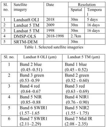
This study was carried out using open sources earth observation datasets such as Landsat 8, Landsat 5, night-time light and SRTM-DEM of 2018, 2009 and 1998 (see table 1 and 2). The Landsat 8, Landsat 5 is openly accessible satellite imageries which were widely used for land use/cover mapping, natural resource management and ecosystem analysis since the past several years. This satellite imagery has a better capability of long-term time series analysis of land use/cover, biodiversity and environment at the local and regional level (Julien et al., 2011; Phiri, et al., 2017). In addition, SRTM-DEM was increasingly used in several studies at regional level land use/cover classification because this helps to differentiate land use/cover classes based on the height variation (Balzter et al., 2015). It is observed that land use/cover with very similar

spectral response located at different altitudes like cropland and vegetation, barren and fallow land etc.

Sl.

no. Satellite imagery Date Spatial TemporaResolution l

1

Landsat8 OLI

2018 30m 5 days

2

Landsat 5 TM

2009 30m 16 days

3

Landsat 5 TM

1998 30m 16 days

4

DMSP-OLS

2018-1998 2.7km

5

SRTM-DEM

30m

Table 1. Selected satellite imageries

Sl. no. Landsat 8 OLI (µm) Landsat 5 TM (µm)

1

Band 2 blue

(0.45–0.51)

Band 1 blue

(0.45 - 0.52)

2

Band 3 green

(0.53–0.59

Band 2 green

(0.52 - 0.60)

3

Band 4 red

(0.64–0.67

Band 3 red

(0.63 - 0.69)

4

Band 5 NIR

(0.85–0.88

Band 4 NIR1

(0.76 - 0.90)

5

Band 6 SWIR1

(1.57–1.65

Band 5 NIR2

(1.55 - 1.75)

6

Band 7 SWIR1

(2.11–2.29)

Band 7 Mid IR

(2.08 - 2.35)

Table 2. Radiometric details of selected satellite imageries The National Oceanic and Atmospheric Administration (NOAA) was launched Defence Meteorological Satellite Program with Operational Linescan System (DMSP-OLS) which provides night-time light imagery to sense light illumination coming from the built-up urban area. The night-time light very helpful for the discrimination of built-up urban area from the non-built-up area (Mustak et al., 2018). This study was carried out using google earth engine, a cloud computing API. This API provided a robust, faster and efficient cloud computing environment for land use/cover classification using open sources satellite imagery. Because, recently Google Earth Engine (GEE) is increasing used for land use/cover mapping and change detection analysis, ecosystem and biodiversity conservation and management and natural resources management (e.g., Jacobson et al., 2015; Julien et al., 2011; Sidhu et al., 2018; Tsai et al., 2018).

2.3 Pre-processing

Pre-processing is an essential step of using remote sensing satellite imagery for several applications like land use/cover mapping etc. In this study, pre-processing includes subsetting, mosaicking and enhancement of the satellite imageries, preparation of training and test samples. Of course, atmospheric and geometric corrections are one of the important steps of pre-processing (Mustak, 2013) but google earth engine has a capability to download radiometrically and geometrically calibrated satellite imagery (Kelley et al., 2018). In addition, mosaic and stacking of images bands during both Kharif and Rabi season were done using median algorithms. The median algorithms (Reducer function) widely used in google earth engine for mosaicking and stacking satellite image bands because it has better capability to represent the central tendency of the variables (e.g., DN values) as compared to other methods e.g., mean, mode (Kelley et al., 2018).

The International Archives of the Photogrammetry, Remote Sensing and Spatial Information Sciences, Volume XLII-3/W6, 2019 ISPRS-GEOGLAM-ISRS Joint Int. Workshop on “Earth Observations for Agricultural Monitoring”, 18–20 February 2019, New Delhi, India

(3)

2.4 Cloud Computing and Machine learning

Google earth engine (GEE) is a cloud computing API which has a better capability to fast access and high computation of large volume of openly accessible satellite imageries (big data) at no cost (Jacobson et al., 2015; Kelley et al., 2018; Tsai et al., 2018). Integration of machine learning algorithms with GEE is an added advantage over advanced machine learning for different application like land use/cover mapping (Tsai et al., 2018). Machine learning algorithms were initially used in computer vision and pattern recognition but recently increasingly used in satellite image classification for environmental monitoring, land use/cover analysis, ecosystem and biodiversity etc. Machine learning algorithms better feasible for analysing pattern from the complex datasets. Because, these algorithms have a better ability for non-linear solution from the complex variables as compared to traditional parametric classification algorithm (e.g., maximum Likelihood classifier) (Mustak, 2018). There are several supervised machine learning algorithms like Support Vector Machine (SVM), Random Forest (RF), Decision Tree (DT), Classification and Regression Tree (CART) etc. were widely explored in different open source and commercial software but in GEE, SVM, RF and CART widely used for land use/cover classification. In this study, SVM with Radial Basis Function (SVM-RBF), RF and CART were used for exploring best machine learning algorithms for land use/cover classification.

2.4.1 Support Vector Machine: Support Vector Machine is one of the robust algorithms of supervised machine learning which was introduced to solve the binary classification problem. In multiclass problem, SVM performs the classification using either one-against-all or one-against-one logical comparison approach and the correct class is then assigned following a voting mechanism (Mazzoni et al., 2007). SVM have several kernel functions linear, polynomial, Gaussian etc. in which Gaussian is robust and widely used. The Gaussian kernel in SVM is called Radial Basis Functions SVM (SVM-RBF). SVM-RBF has two important kernel parameters such as cost and gamma. The cost parameter explained the penalty to reduce the slack variables while gamma parameter is the bandwidth of the Gaussian kernel. Higher the value of cost, maximum penalty on slack variables and similarly, higher the value of gamma, higher is the biases (e.g., low variance) and vice versa (Mustak, 2018). Optimum size of cost and gamma helps to reduce the overfitting of the algorithms and maximizing the overall classification accuracy. To obtain the optimal size of cost and gamma, grid search parameter tuning approach with k-fold cross-validation widely used ( Mustak, 2018; Tsai et al., 2018). The range of cost is

10

1

to 10

2

and

gamma is 10

-2

to 10

1

was selected for parameter tuning of

SVM-RBF.

2.4.2 Random Forest: Random Forest (RF) is a deep tree model which known as ensemble learning technique developed by Breiman (2001) to improve the classification and regression of trees (CART) (Adam et al., 2014). It is a combination of large set of decision trees and each tree contribute a single vote for the most frequent class (Adam et al., 2014; Lin et al., 2010). This algorithm benefitted by two techniques such as bagging and random subspace selection (Adam et al., 2014; Lin et al. 2010) In RF, there are two important parameters and processes such as ntree and bootstrap sampling, and mtry and node splitting. In ntree and bootstrap sampling, bootstrap samples

were drawn from the original datasets to builds many binary classification trees (ntree). These bootstrap samples also called as the out-of-bag samples which used for approximation of validation errors to sort out optimum number of ntree (Adam et al., 2014). However, the classification trees as builds from bootstrap samples contribute a unit vote and each unit vote for the correct classification is determined by the majority vote from all the trees in the forest (Adam et al., 2014). Thus, in mtry and node splitting process, each node is assigned by the given number of input variables (mtry) which randomly selected from the random subset of features. These random subsets of features are utilized for splitting best node (Adam et al., 2014). It very important to adopt best strategy (e.g., parameter tuning) to select best ntree and mtry in RF to obtain more stabilize and de-correlated classification tree for robust classification outcome. In RF, parameter tuning was mostly used for selecting best ntree instead of mtry (often default performs best) because overall classification accuracy highly affected by the size of ntree ( Adam et al., 2014; Thanh Noi & Kappas, 2017).

2.4.2 Classification and Regression Tree: The classification and regression tree (CART) is a known as decision tree (DT). DT is a kind of chain-like decision support system in supervised machine learning based on some logical inferences (e.g., if-else-then, greater than-less than etc.) drawn from statistical parameters (e.g., entropy). Based on some logical inference drawn from statistical parameters, the training attributes (parent node) splitting into child node (classification tree) to obtain leaf node (final test class/regression tree) using recursive computational approach (Oliveira et al., 2017; Laliberte & Rango, 2009; Wu et al., 2007). Parameter tuning (e.g., depth of tree etc.) is sometime applied for reducing the overfitting of the classifier to improve the classification accuracy but default parameters of CART in GEE normally provided higher overall classification accuracy.

2.5 Land use/cover classification scheme

In this study, land use/cover classes were selected based on local land use classification scheme, local context and literature reviews. Following land use/cover classes were selected such as:

1. Built-up- urban and rural built-up.

2. Cropland- Kharif and Rabi, agricultural plantation. 3. Fallow land- Kharif and Rabi fallow.

4. Vegetation-forest, trees, forest plantation. 5. Scrub and grassland-grazing land, bushes etc. 6. Barren and sandy land- exposed rock, waste lands,

river bank, river sand etc.

7. Water Bodies- tank, pond, lake, river etc.

2.6 Selection of Training and test samples

Selection of training and test samples is one of the important steps to explain the uncertainty in image classification. In image classification, there are several approaches like binomial minimum fifty sample rules were adopted by many researchers to select the optimum number of training samples (Foody, 2009). Lack of optimum number of training samples in image classification is largely affected by the Hughes phenomena (Damodaran et al., 2017). In many studies, minimum fifty sample rule was widely used in image classification for land use/cover and biodiversity applications (e.g., Foody, 2009). In this study, minimum fifty sample rule was adopted to randomly select the training samples using simple random sampling in The International Archives of the Photogrammetry, Remote Sensing and Spatial Information Sciences, Volume XLII-3/W6, 2019 ISPRS-GEOGLAM-ISRS Joint Int. Workshop on “Earth Observations for Agricultural Monitoring”, 18–20 February 2019, New Delhi, India

(4)

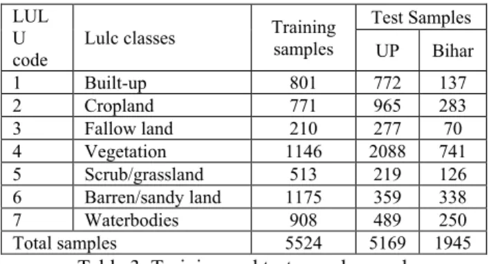
GEE (see table 3). The training samples were splitting into training and validation samples during feature selection and parameters tuning using 60 (training) and 40 (validation) percent rules. In addition, 5169 test samples for UP and 1945 test samples for Bihar were randomly selected to validate and final accuracy assessment using GEE (see table 3).

LUL U

code Lulc classes

Training samples Test Samples UP Bihar 1 Built-up 801 772 137 2 Cropland 771 965 283 3 Fallow land 210 277 70 4 Vegetation 1146 2088 741 5 Scrub/grassland 513 219 126 6 Barren/sandy land 1175 359 338 7 Waterbodies 908 489 250 Total samples 5524 5169 1945

Table 3. Training and test samples used

2.7 LULC Classification

Land use/cover classification using satellite imageries is very essential to adopt the following steps for robust outcome. In this study, pixel-based classification approach was employed because this approach was widely used for land use/cover classification. Following steps were adopted for the classification of land use/cover, such as:

2.7.1 Feature extraction and normalization: Following image features were extracted (see table 4) based on the literature survey such as:

• Spectral bands: six spectral image bands as mentioned in the table 2 were selected because such spectral image bands were commonly used in many studies for land use/cover classification (Mandanici & Bitelli, 2016) This is because such spectral bands have better class separability ability for land/cover classification as compared to all image bands.

• Normalized Difference Vegetation Index: Normalized Difference Vegetation Index (NDVI) commonly used in land use/cover classification for discrimination of vegetated area from the non-vegetated area (Kelley et al., 2018). NDVI was calculated using following equation 1:

NDVI value is varied from +1 to -1 which explained that the area having NDVI value +1 is explained the area having highly vegetated area. Inversely, NDVI value -1 explained the area having highly non-vegetated area.

Image Features Number

Spectral bands 06 NDVI 01 GLCM 06 DEM 01 Night-time light 01 Total 15

Table 4. Extracted image features

• Grey Level Co-occurrence Matrix: Gray Level Co-occurrence Matrix (GLCM) is used to extract texture features. The texture feature is added advantages over the

spectral image features to improve the overall classification accuracy (Chuang & Shiu, 2016). Because, sometimes distinct land use/cover objects have also distinct texture along with similar spectral response. In this study, GLCM mean in all direction with 4-by-4 kernel was calculated using equation 2.

GLCM mean was widely used in land use/cover classification from the high resolution satellite imagery (Mustak, 2018) but it was also used in medium resolution satellite imagery (Sothe et al., 2017).

• Digital Elevation Model: Digital Elevation Model (DEM) one of the very important features for land use/cover classification for the area which is mixed with plain and elevated landscape (Balzter et al., 2015; Manandhar et al., 2009). Because, locational variation of land use/cover ideally related to the variation of elevation although having similar spectral and textural response.

• Night-time light: NOAA launched the Defence Meteorological Satellite Program with Operational Linescan System (DMSP-OLS) which provided night-time light satellite imagery (Mustak et al., 2018). The night-time light satellite imagery capable to distinguish from built-up urban from the rural areas based on light illumination (Mustak et al., 2018).

All the image features were normalized using max-min method which value is varied from 0 to 1. The normalization of image features is very important for standardizing all features into a standard scale which is very helpful for reducing uncertainty in the training process.

2.7.2 Features selection and parameter tuning:

Feature selection is another important step in image classification which was commonly used in land use/cover mapping. The features selection is used for dimensionality reduction for selecting best image features which have maximum class separability (Camps-valls, et al., 2010). In image classification, several feature selection methods such as Principal component Analysis (PCA), rank, regression, sequential etc. were adopted but sequential feature selection approach is robust and faster as compared to the others (Camps-valls, et al., 2010; Mustak, 2018). In this study, sequential feature selection approach was employed and developed in GEE. In addition, feature selection also very important for reducing the effects of Hughes phenomena (Ma et al., 2013). Beyond the feature selection, parameter tuning is also important consideration to reduce the overfitting of classifiers (Tsai et al., 2018). The parameter tuning of SVM-RBF (e.g., cost, gamma) was carried using holdout K-fold (e.g., 10 fold) cross-validation with grid search method while holdout K-fold (e.g., 10 fold) cross-validation employed for parameter (e.g., ntree) tuning of Random forest. Feature selection and parameters tuning were carried out over UP and best features and parameters were used for both the UP and Bihar for land use/cover classification.

2.7.3 Sensitivity analysis on size of training samples: Beyond the selection of best features and best parameters, selection of the optimal size of training samples is another important step in image classification. Selection of optimal size of training samples is essential to reduce the effect of Hughes phenomena (Ma et al., 2015; Thanh Noi & Kappas, 2017). The The International Archives of the Photogrammetry, Remote Sensing and Spatial Information Sciences, Volume XLII-3/W6, 2019 ISPRS-GEOGLAM-ISRS Joint Int. Workshop on “Earth Observations for Agricultural Monitoring”, 18–20 February 2019, New Delhi, India

(5)

training samples were evaluated by randomly splitting into four parts in percent basis such as 25%, 50%, 75% and 100% and testify with 5169 test samples. Selection of the optimal size of training samples were carried out over UP and selected optimal size of training samples were used for both the UP and Bihar to train and classify the land use/cover.

2.7.4 Classification and accuracy assessment:

In this study, three machine learning algorithms such as SVM-RBF, RF and CART for land use/cover classification. Best features, best parameters and optimum size of training samples were optimized to train the classifiers over UP in 2018. Finally, trained models of different classifiers were used to classify the land use/cover of both the UP and Bihar over different decades. The classified land use/cover maps of UP and Bihar were used for final accuracy assessment using confusion matrix and quantify with overall accuracy and kappa indices. The overall accuracy explained the pixel correctly matched with classified and referenced land use/cover maps while kappa was used to assess the random error on overall classification accuracy.

2.7.5 Transferability analysis: transferability is the term generally used when model is train over one segment and tested over another segment. Transferability is usually used to generalize the model (Wieland & Pittore, 2014). The spatial transferability is called when model is train over one area and tested over another area. In this study, model was train over UP and tested over Bihar to assess the spatial transferability. In addition, model was train over UP in 2018 and tested over Bihar in different decades (e.g., 2018, 2009, 1998) to assess the temporal transferability.

3. RESULTS AND DISCUSSIONS

Based on the several employed scientific methods following results have obtained to address the research objective of this article. The results explained in the following sub-sections:

3.1 Best features

Feature selection was employed using SVM-RBF. Based on the sequential feature selection approach, 15 image features in including image bands, GLCM mean, NDVI, DEM and night-time light shows higher overall accuracy (96.70%) as compared to others set of image features(see figure 1). Only using the image bands, the overall accuracy was 93.93% and slightly improves to 95.03% while NDVI added with image bands. Thus, while GLCM added with image bands and NDVI, the overall accuracy increases to 95.47%. This shows that textural and contextual information are very necessary along with image bands to improve the classification accuracy. It is also observed that while nigh-time light was added with image bands, GLCM and NDVI, the overall accuracy was decreased to 90.85%. In addition, while DEM added with image bands, NDVI, GLCM and night-time light the overall accuracy rapidly increased to 96.70% because height information is very essential to discriminate different land use/cover in semi-elevated landscape.

3.2 Best parameters

The hold out 10-fold cross-validation and grid search were employed for parameter tuning. The results show that cost is 10 and gamma is 1.20 are the best parameters of SVM-RBF which provides 96.70% overall classification accuracy as compared to others fold of parameters. In addition, 64 nTree are the best parameters of RF which provides 90.24% as compared to others fold of nTree.

3.3 Optimal size of training samples

The sensitivity analysis of training samples was carried on SVM-RBF using best features, parameters and tested over full test samples (see table 5). The result shows that use of inappropriate size of training samples affected the overall classification accuracy. Sufficient size (5524) of training samples always necessary to reduce the effects of Hughes phenomena and to improve the overall classification accuracy.

Size of training

samples Overall accuracy (%) Kappa (%)

40%

95.57

94.16

60%

95.14

93.62

80%

97.47

96.67

100%

98.61

98.17

Table 5. Selection of optimum size of training samples

3.4 Classification and accuracy assessment

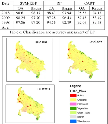
Final classification results shows in figure 2, 3 and table 6 and 7. The results shows that classification accuracy is higher for SVM-RRF as compared to RF and CART both in UP and Bihar. In addition, the results also show that overall accuracy is high in UP while low in Bihar due to increases of uncertainty in transferability of model parameters.

Date SVM-RBF RF CART

OA Kappa OA Kappa OA Kappa

2018 98.61 98.17 98.43 97.94 95.53 94.13 2009 98.25 97.70 97.28 96.43 87.43 83.49 1998 97.86 97.20 94.56 92.89 92.06 89.65 Ave.

Table 6. Classification and accuracy assessment of UP

Figure 2. Classified map of UP using SVM-RBF The International Archives of the Photogrammetry, Remote Sensing and Spatial Information Sciences, Volume XLII-3/W6, 2019 ISPRS-GEOGLAM-ISRS Joint Int. Workshop on “Earth Observations for Agricultural Monitoring”, 18–20 February 2019, New Delhi, India

(6)

The results also show that classification accuracy is decreasing with change of decades due to uncertainty increase in transferring of model parameters.

2018 96.30 95.21 92.44 90.29 82.67 78.19 2009 97.29 96.44 90.78 87.64 80.60 74.34 1998 95.86 94.87 85.29 81.87 75.14 70.06 Ave.

Table 7. Classification and accuracy assessment of Bihar

3.5 Transferability analysis

The transferability analysis explained how model can be trained over one place or one time and can be employed over different areas and times. This helps to generalize the classification results. The results show that SVM-RBF has better spatial and temporal transferability ability as compared to other classifiers (see table 8). Thus, SVM-RBF is more robust and has better generalization ability as compared to others machine learning classifiers.

2018 97.46 96.69 95.44 94.12 89.10 86.16 2009 97.77 97.07 94.03 92.04 84.02 78.92 1998 96.86 96.04 89.93 87.38 83.60 79.86 Ave. 97.36 96.60 93.13 91.18 85.57 81.64 Table 8. Transferability analysis of machine learning algorithms

3.6 Conclusion and recommendation

Land use/cover classification from satellite images widely explored in many researches using machine learning algorithms but very limited study explored machine learning algorithms with cloud computing API. In addition, generalization of the classification is very essential which rarely carried in many researches. This study is very helpful to apply for land use/cover classification across larger area and different temporal dimension using robust classification algorithm. In addition, this study provides polishing guideline for selecting appropriate image features, parameters, and machine learning

classifiers feasible on cloud computing API. This study is tested over two states of India with random test samples for generalize the machine learning algorithms which is sometime more or less biased for large area. In this regard, to obtain unbiased and transparent outcome for larger area it is recommended to test over more states with full reference land use/cover map.

ACKNOWLEDGEMENTS

I very thankful to University Grants Commissions, New Delhi, India for providing fellowship to complete this research.

REFERENCES

Adam, E., Mutanga, O., Odindi, J., & Abdel-Rahman, E. M., 2014. Land-use/cover classification in a heterogeneous coastal landscape using RapidEye imagery: evaluating the performance of random forest and support vector machines classifiers. International Journal of Remote Sensing, 35(10), pp. 3440– 3458. https://doi.org/10. 1080/ 01431161.2014.903435.

Balzter, H., Cole, B., Thiel, C., Schmullius, C., Balzter, H., Cole, B., Schmullius, C., 2015. Mapping CORINE Land Cover from Sentinel-1A SAR and SRTM Digital Elevation Model Data using Random Forests. Remote Sensing, 7(11), pp. 14876– 14898. https://doi.org/10.3390/ rs71114876.

Breiman, L., 2001. Random Forests. Machine Learning, 45(1), pp. 5–32. https://doi.org/10.1023/A:1010933404324.

Camps-valls, G., Mooij, J., & Schölkopf, B., 2010. Kernel Dependence Measures. IEEE Geoscience and Remote Sensing Letters, 7(3), pp. 587–591.

Chuang, Y.C., & Shiu, Y.S., 2016. A Comparative Analysis of Machine Learning with WorldView-2 Pan-Sharpened Imagery for Tea Crop Mapping. Sensors, 16(5), pp. 594. https://doi.org/10.3390/s16050594.

Damodaran, B. B., Courty, N., & Lefevre, S., 2017. Sparse Hilbert Schmidt Independence Criterion and Surrogate-Kernel-Based Feature Selection for Hyperspectral Image Classification. IEEE Transactions on Geoscience and Remote Sensing, 55(4), pp. 2385–2398. https://doi.org/ 10.1109/TGRS.2016.2642479. Foody, G. M., 2009. Sample size determination for image classification accuracy assessment and comparison. In: International Journal of Remote Sensing, 30(20), pp. 5273– 5291. https://doi.org/10.1080/01431160903130937.

Foody, G. M., & Mathur, A., 2004a. A relative evaluation of multiclass image classification by support vector machines. IEEE Transactions on Geoscience and Remote Sensing, 42(6), pp. 1335–1343. https://doi.org/ 10.1109/ TGRS.2004.827257. Foody, G. M., & Mathur, A., 2004b. Toward intelligent training of supervised image classifications: directing training data acquisition for SVM classification. Remote Sensing of Environment, 93(1–2), pp. 107–117. https:// doi.org/ 10.1016/J.RSE.2004.06.017.

Grimm, N. B., Foster, D., Groffman, P., Grove, J. M., Hopkinson, C. S., Nadelhoffer, K. J., Peters, D. P., 2008. The changing landscape: ecosystem responses to urbanization and Figure 3. Classified map of Bihar using SVM-RBF

(7)

pollution across climatic and societal gradients. Frontiers in Ecology and the Environment, 6(5), pp. 264–272. https://doi.org/10.1890/070147.

Hong, J.H., Min, J.K., Cho, U.K., & Cho, S.B., 2008. Fingerprint classification using one-vs-all support vector machines dynamically ordered with naı¨ve Bayes classifiers. Pattern Recognition, 41(2), pp. 662–671. https://doi.org/10.1016/j.patcog.2007.07.004.

Islam, T., Rico-Ramirez, M. A., Han, D., & Srivastava, P. K., 2012. Artificial intelligence techniques for clutter identification with polarimetric radar signatures. Atmospheric Research, pp.

109–110, 95–113. https://doi.org/

10.1016/J.ATMOSRES.2012.02.007.

Jacobson, A., Dhanota, J., Godfrey, J., Jacobson, H., Rossman, Z., Stanish, A., Riggio, J., 2015. A novel approach to mapping land conversion using Google Earth with an application to East Africa. Environmental Modelling & Software, 72, pp. 1–9. https://doi.org/10.1016/ J.ENVSOFT. 2015.06.011.

Julien, Y., Sobrino, J. A., & Jiménez-Muñoz, J.C., 2011. Land use classification from multitemporal Landsat imagery using the Yearly Land Cover Dynamics (YLCD) method. International Journal of Applied Earth Observation and Geoinformation, 13(5), pp. 711–720. https://doi.org/ 10.1016/J.JAG.2011.05.008.

Kelley, L. C., Pitcher, L., Bacon, C., Kelley, L. C., Pitcher, L., & Bacon, C., 2018. Using Google Earth Engine to Map Complex Shade-Grown Coffee Landscapes in Northern Nicaragua. Remote Sensing, 10(6), pp. 952. https://doi.org /10.3390/rs10060952.

Laliberte, A. S., & Rango, A., 2009. Texture and scale in object-based analysis of subdecimeter resolution unmanned aerial vehicle (UAV) imagery. IEEE Transactions on Geoscience and Remote Sensing, 47(3), pp. 1–10. https://doi.org/10.1109/TGRS.2008.2009355.

Lau, K. W., & Wu, Q. H., 2008. Local prediction of non-linear time series using support vector regression. Pattern Recognition, 41(5), pp. 1539–1547. https://doi.org/10.1016/ J.PATCOG.2007.08.013.

Lin, X., Sun, L., Li., Y., Guo, Z., Li, Y., Zhong, K., Xu, G., 2010. A random forest of combined features in the classification of cut tobacco based on gas chromatography fingerprinting. Talanta, 82(4), pp. 1571–1575. https://doi.org/10.1016/J.TALANTA.2010.07.053.

Ma, L., Cheng, L., Li, M., Liu, Y., & Ma, X., 2015. Training set size, scale, and features in Geographic Object-Based Image Analysis of very high resolution unmanned aerial vehicle imagery. ISPRS Journal of Photogrammetry and Remote Sensing, 102, pp. 14–27. https://doi.org/10.1016/ j.isprsjprs.2014.12.026.

Ma, W., Gong, C., Hu, Y., Meng, P., & Xu, F., 2013. The Hughes phenomenon in hyperspectral classification based on the ground spectrum of grasslands in the region around Qinghai Lake. In: International Symposium on Photoelectronic Detection and Imaging 2013: Imaging Spectrometer Technologies and Applications, 8910(August 2013), 89101G. https://doi.org/10.1117/ 12.2034457.

Man, Q., Dong, P., & Guo, H., 2015. Pixel- and feature-level fusion of hyperspectral and lidar data for urban land-use classification. International Journal of Remote Sensing, 36(March), pp. 1618–1644. https://doi.org/10.1080/ 014311 61.2015.1015657.

Manandhar, R., Odehi, I. O. A., & Ancevt, T., 2009. Improving the accuracy of land use and land cover classification of landsat data using post-classification enhancement. Remote Sensing, 1(3), pp. 330–344. https://doi.org/ 10.3390/rs1030330.

Mandanici, E., & Bitelli, G., 2016. Preliminary comparison of sentinel-2 and landsat 8 imagery for a combined use. Remote Sensing, 8(12). https://doi.org/10.3390/ rs8121014.

Mazzoni, D., Garay, M. J., Davies, R., & Nelson, D., 2007. An operational MISR pixel classifier using support vector machines. Remote Sensing of Environment, 107(1–2), pp. 149– 158. https://doi.org/10.1016/J.RSE.2006.06.021.

Mustak, S., 2013. Correction Of Atmospheric Haze In Resourcesat-1 Liss-4 Mx Data For Urban Analysis: An Improved Dark Object Subtraction Approach. In: ISPRS - International Archives of the Photogrammetry, Remote Sensing and Spatial Information Sciences, XL-1/W3, pp. 283–287. https://doi.org/10.5194/isprsarchives-XL-1-W3-283-2013. Mustak, S., 2018. Evaluating The Performance Of Machine Learning Algorithms For Urban Land Use Mapping Using Very High Resolution. University Of Twente. Retrieved from https://library.itc.utwente.nl/papers_2018/msc/upm/sheikh.pdf. Mustak, S., Baghmar, N. K., Srivastava, P. K., Singh, S. K., & Binolakar, R., 2018. Delineation and classification of rural– urban fringe using geospatial technique and onboard DMSP– Operational Linescan System. Geocarto International, 33(4), pp. 375–396. https://doi.org/10.1080/ 10106049.2016.1265594. Oliveira Silveira, E. M., de Menezes, M. D., Acerbi Júnior, F. W., Castro Nunes Santos Terra, M., & de Mello, J. M., 2017. Assessment of geostatistical features for object-based image classification of contrasted landscape vegetation cover. Journal of Applied Remote Sensing, 11(3), 036004. https://doi.org/10.1117/1.JRS.11.036004.

Pal, M., & Mather, P. M., 2004. Assessment of the effectiveness of support vector machines for hyperspectral data. Future Generation Computer Systems, 20(7), pp. 1215–1225. https://doi.org/10.1016/J.FUTURE.2003.11.011

Patel, D. P., Gajjar, C. A., & Srivastava, P. K., 2013. Prioritization of Malesari mini-watersheds through morphometric analysis: a remote sensing and GIS perspective. Environmental Earth Sciences, 69(8), pp. 2643–2656. https://doi.org/10.1007/s12665-012-2086-0.

Phiri, D., Morgenroth, J., Phiri, D., & Morgenroth, J., 2017. Developments in Landsat Land Cover Classification Methods: A Review. Remote Sensing, 9(9), pp. 967. https://doi.org/10.3390/rs9090967.

Seto, K. C., & Kaufmann, R. K., 2005. Using logit models to classify land cover and land‐cover change from Landsat Thematic Mapper. International Journal of Remote Sensing, 26(3), pp. 563–577. https://doi.org/10.1080/ The International Archives of the Photogrammetry, Remote Sensing and Spatial Information Sciences, Volume XLII-3/W6, 2019 ISPRS-GEOGLAM-ISRS Joint Int. Workshop on “Earth Observations for Agricultural Monitoring”, 18–20 February 2019, New Delhi, India

(8)

01431160512331299270.

Shao, Y., & Lunetta, R. S., 2012. Comparison of support vector machine, neural network, and CART algorithms for the land-cover classification using limited training data points. ISPRS Journal of Photogrammetry and Remote Sensing, 70, pp. 78– 87. https://doi.org/10.1016/j.isprsjprs. 2012.04.001.

Sidhu, N., Pebesma, E., & Câmara, G., 2018. Using Google Earth Engine to detect land cover change: Singapore as a use case. European Journal of Remote Sensing, 51(1), pp. 486–500. https://doi.org/10.1080/22797254.2018.1451782.

Singh, N. J., Kudrat, M., Jain, K., & Pandey, K., 2011. Cropping pattern of Uttar Pradesh using IRS-P6 (AWiFS) data. International Journal of Remote Sensing, 32(16), pp. 4511– 4526. https://doi.org/10.1080/ 01431161. 2010.489061.

Singh, S. K., Laari, P. B., Mustak, S., Srivastava, P. K., & Szabó, S., 2017. Modelling of land use land cover change using earth observation data-sets of Tons River Basin, Madhya Pradesh, India. Geocarto International, 6049(July), pp. 1–21. https://doi.org/10.1080/ 10106049. 2017.1343390.

Singh, S. K., Mustak, S., Srivastava, P. K., Szabó, S., & Islam, T., 2015. Predicting Spatial and Decadal LULC Changes Through Cellular Automata Markov Chain Models Using Earth Observation Datasets and Geo-information. Environmental Processes, 2(1), pp. 61–78. https://doi.org/ 10.1007/s40710-015-0062-x.

Sothe, C., de Almeida, C. M., Liesenberg, V., & Schimalski, M. B., 2017. Evaluating Sentinel-2 and Landsat-8 data to map sucessional forest stages in a subtropical forest in Southern Brazil. Remote Sensing, 9(8). https://doi.org/ 10.3390/rs9080838.

Thanh Noi, P., & Kappas, M., 2017. Comparison of Random Forest, k-Nearest Neighbor, and Support Vector Machine Classifiers for Land Cover Classification Using Sentinel-2 Imagery. Sensors, 18(1), pp. 18. https://doi.org/ 10.3390/s18010018.

Tsai, Y., Stow, D., Chen, H., Lewison, R., An, L., Shi, L., Shi, L., 2018. Mapping Vegetation and Land Use Types in Fanjingshan National Nature Reserve Using Google Earth Engine. Remote Sensing, 10(6), pp. 927. https://doi.org/10.3390/rs10060927.

Vapnik, V. N., 2000. Introduction: Four Periods in the Research of the Learning Problem. In The Nature of Statistical Learning Theory, pp. 1–15. New York, NY: Springer New York. https://doi.org/10.1007/978-1-4757-3264-1_1.

Vapnik, V. N., & Chervonenkis, A. Y., 1971. On the Uniform Convergence of Relative Frequencies of Events to Their Probabilities. Theory of Probability & Its Applications, 16(2), pp. 264–280. https://doi.org/10.1137/1116025.

Wieland, M., & Pittore, M., 2014. Performance evaluation of machine learning algorithms for urban pattern recognition from multi-spectral satellite images. Remote Sensing, 6(4), pp. 2912– 2939. https://doi.org/10.3390/ rs6042912.

Wu, S., Silvánhyphen;Cárdenas, J., & Wang, L., 2007. Per‐field urban land use classification based on tax parcel

boundaries. International Journal of Remote Sensing, 28(12), pp. 2777–2801. https://doi.org/10.1080/ 0143116 0600981541.