Moderate deviations principle and importance sampling for slow-fast diffusions with small noise

(1)

Boston University

OpenBU http://open.bu.edu

Theses & Dissertations Boston University Theses & Dissertations

2019

Moderate deviations principle and

importance sampling for slow-fast

diffusions with small noise

https://hdl.handle.net/2144/34916

(2)

BOSTON UNIVERSITY

GRADUATE SCHOOL OF ARTS & SCIENCES

Dissertation

MODERATE DEVIATIONS PRINCIPLE AND

IMPORTANCE SAMPLING FOR SLOW–FAST

DIFFUSIONS WITH SMALL NOISE

by

MATTHEW R. MORSE

B.S., Harvey Mudd College, 1995

M.A., Boston University, 2014

Submitted in partial fulfillment of the

requirements for the degree of

Doctor of Philosophy

(3)

c

2019 by

(4)

Approved by

First Reader

Konstantinos Spiliopoulos, PhD

Associate Professor of Mathematics and Statistics

Second Reader

Solesne Bourguin

Assistant Professor of Mathematics and Statistics

Third Reader

Michael Salins

Assistant Professor of Mathematics and Statistics

Fourth Reader

Ting Zhang

(5)

Acknowledgments

I would like to thank my advisor, Kostas Spiliopoulos, for all of his guidance and assistance of the past several years. I would like to thank the professors and the other graduate students of the Department of Mathematics and Statistics for the supportive and encouraging work environment. I would like to thank the Department of Mathematics and Statistics at the University of Maine, where I have been located during my final semester completing this dissertation, for giving me the necessary time and space to do this work. I would like to thank my friends and family, both for their support and for their understanding when I have not always been available to them.

This dissertation represents the culmination of a very long process and I would like to thank some individuals specifically for their role early in this process. I would like to thank Benoit Mandelbrot, despite the fact that I never had an opportunity to meet or interact with him. Experimenting with the Mandelbrot set when I should have been doing much less interesting work at my job reminded me of my love of mathematics and first led me to consider graduate work in mathematics. I would like to thank Kate Thornton for suggesting that I study statistics. In retrospect it is obvious that probability and statistics is my field, but until she suggested it, that possibility had not occurred to me. Finally, I would like to thank Daniel Weiner. He was one of my instructors when I was first getting my feet wet in studying statistics, and his advice and assistance provided essential steps on my path to where I am today.

(6)

MODERATE DEVIATIONS PRINCIPLE AND

IMPORTANCE SAMPLING FOR SLOW–FAST

DIFFUSIONS WITH SMALL NOISE

MATTHEW R. MORSE

Boston University, Graduate School of Arts & Sciences, 2019

Major Professor: Konstantinos Spiliopoulos, PhD

Associate Professor of Mathematics and Statistics

ABSTRACT

We prove the moderate deviations principle (MDP) for a general system of slow-fast dynamics. We provide a unified approach, based on weak convergence ideas and stochastic control arguments, that cover both the averaging and the homogenization regimes. We allow the coefficients to be in the whole space and not just the torus and allow the noises driving the slow and fast processes to be correlated arbitrarily.

We then construct provably logarithmic asymptotically optimal importance sam-pling schemes for the estimation of rare events based on the moderate deviations principle. Using the subsolution approach we construct schemes and identify condi-tions under which the schemes will be asymptotically optimal. Moderate deviacondi-tions based importance sampling offers a viable alternative to large deviations importance sampling when the events are not too rare. In particular, in many cases of interest one can indeed construct the required change of measure in closed form, a task which is more complicated using the large deviations based importance sampling, especially when it comes to multiscale dynamically evolving processes. The presence of mul-tiple scales and the fact that we do not make any periodicity assumptions for the

(7)

coefficients driving the processes complicate the design and the analysis of efficient importance sampling schemes. Simulation studies illustrate the theory.

(8)

List of Tables

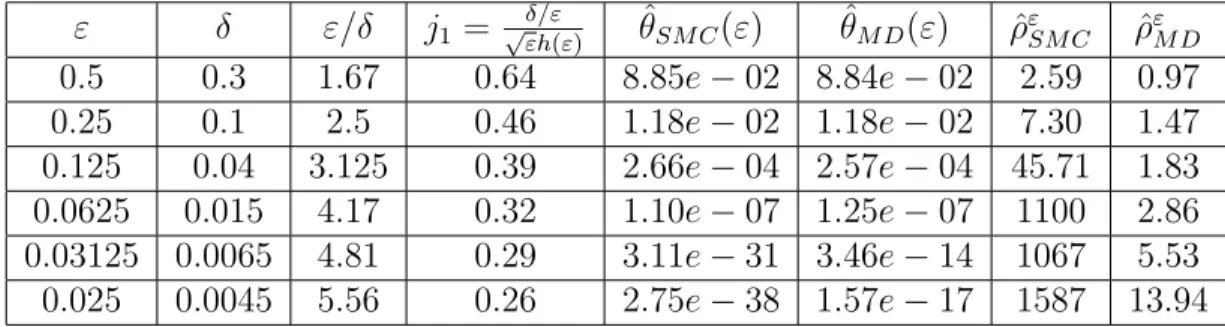
3.1 Comparison table for slow-fast system in Regime 2. . . 64

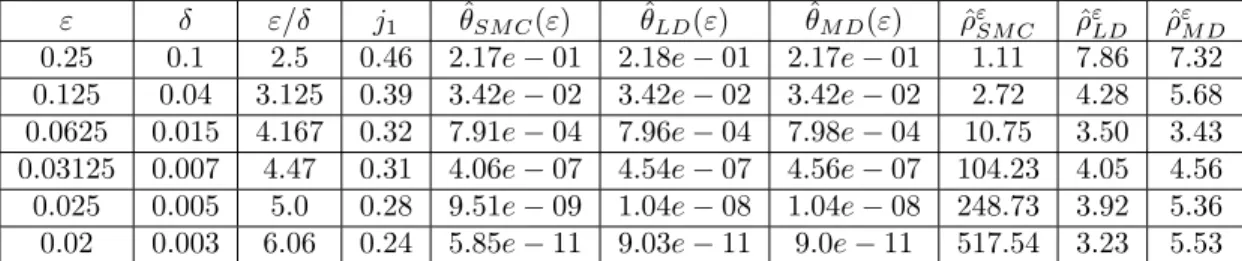
3.2 Comparison table for 2-d slow fast system in Regime 1. . . 68

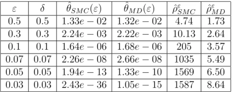
3.3 Comparison table for 2-d slow fast system in Regime 2. . . 68

(12)

Chapter 1

Introduction

1.1

Multiscale Diffusion Processes

In this dissertation we study moderate deviations and importance sampling for mul-tiscale diffusion processes with small noise of the form

dX_tε=hε δb(X ε t, Y ε t ) +c(X ε t, Y ε t ) i dt+√εσ(X_tε, Y_tε)dWt (1.1) dY_tε= 1 δ hε δf(X ε t, Y ε t) +g(X ε t, Y ε t ) i dt+ √ ε δ [τ1(X ε t, Y ε t )dWt+τ2(Xtε, Y ε t )dBt] X₀ε =x0, Y0ε =y0

fort∈[0, T] such that (Xε

t, Ytε)∈Rn×Rd. For convenience, we refer to the state space

of Yε _as _Y_{. The parameter} _ε _{1 represents the strength of the noise while} _δ ₁

is the time-scale separation parameter. Wt and Bt are independent m-dimensional

Brownian motions.

Multiscale models of the form (1.1) appear in applications in many branches of science. Examples include protein folding models in molecular biology (Zwanzig, 1988), seizure dynamics models in neuroscience (Jirsa et al., 2014), stock price models in economics (Feng et al., 2012), and teleconnections in climate dynamics (Majda et al., 2008). Due to the structure of the SDEs, closed form analytic solutions are not available and we must rely on approximations or numeric approaches.

(13)

scales, i.e.,

dX_tε=b(X_tε)dt+√εσ(X_tε)dWt

have been extensively studied, for example (Freidlin and Wentzell, 1984; Baier and Freidlin, 1977; Freidlin, 1978). The multiscale setting significantly complicates the analysis, and the goal of this work is to develop similar results for this setting.

1.2

Applications of Multiscale Models

As stated above, multiscale models arise in a variety of applications. We present examples here as motivation for the general study of multiscale processes, which is the focus of this dissertation.

1.2.1 Protein Folding Models

(Zwanzig, 1988) presents a multiscale model as a hypothetical tool for studying the dynamics of protein folding. The potential surface of a protein is expected to have a hierarchical structure, with many local minima and small potential barriers that must be traversed to reach a large scale minimum. At low temperatures, diffusion will be hampered by the barriers. The model decomposes the potential function U(x) into a smooth background functionU0(x) and a rapidly oscillating perturbationU1(x), with

typical amplitude ε and typical length scale δ. The stochastic differential equation for the state can be written as a first order Langevin equation,

dXt = −ε δ∇U1 Xt δ − ∇U0(Xt) dt+√ε√2DdWt, X0 =x0,

where D is a diffusion constant corresponding to the temperature of the system. By introducing the variable Yt=Xt/δ, this can be expressed in the form of (1.1).

(14)

1.2.2 Seizure Dynamics Models

In a seizure, large regions of the brain produce uncontrolled synchronous neural activ-ities. An experimental model for brain seizures based on five state variables has been developed with the goal of identifying rules governing the initiation of seizures (Jirsa et al., 2014). Two state variables are responsible for generating rapid discharges and operate at a fast time scale. Two variables generate spike and wave events and oper-ate at an intermedioper-ate time scale. Finally, one slow variable models the alternation between “normal” and ictal periods. These five variables (at three time scales) satisfy the following system of equations.

˙ x1 =y1−f1(x1, x2)−z+lrest1 ˙ y1 =y0−5x21 −y1 ˙ z= 1 τ0 (4(x1−x0)−z) ˙ x2 =−y2+x2−x32+lrest2+ 0.002g(x1)−0.3(z−3.5) ˙ y2 = 1 τ2 (−y2+f2(x1, x2))

In these equations, τ0 = 2857 and τ2 = 10 are time–scale separation constants.

The variables x1 and y1 are the fast variables, x2 and y2 are the intermediate scale

variables, andz is the slow variable. Noise is introduced into each equation as Gaus-sian white noise with zero mean and variance of 0.025 for the fast subsystem and 0.25 for the intermediate subsystem.

1.2.3 Financial Pricing Models

Stochastic volatility models have been used to study the behavior of short maturity options. In models with a fast mean-reverting stochastic volatility factor, this leads to a multiscale model. (Feng et al., 2012) study the evolution of a stock price St with

(15)

stochastic volatility Yt given by dSt =rStdt+σ(Yt)StdW (1) t dYt = 1 δ(m−Yt)dt+ ν √ δY β t dW (2) t

Studying the behavior of this process on short time scales leads to a rescaling, after which these equations take the form of (1.1).

1.2.4 Climate Dynamics Models

Atmospheric general circulation models, used for weather prediction and climate mod-eling, typically involve thousands of variables. Northern Hemisphere low–frequency climate variability can be described by only a few teleconnection patterns. In order to produce computationally efficient results, (Majda et al., 2008) proposes a model for these teleconnections involving only four variables. Two variables,x1 and x2,

rep-resent large scale climate modes, whiley1 and y2 represent synoptic weather systems

or convection. The model has the form

dx1 = ((−x2(L12+a1x1+a2x2) +d1x1+F1) +L13y1+b123x2y1)dt dx2 = ((+x1(L21+a1x1+a2x2) +d2x2+F2) +L24y2+b213x1y1)dt dy1 = −L13x1+b312x1x2+F3− γ1 ε y1 dt+√σ1 εdW1 dy2 = −L24x2+F4− γ2 ε y2 dt+√σ2 εdW2

(16)

1.3

Moderate Deviations and Connections to Large

Devia-tions

The study of moderate deviations amounts to a rescaling of large deviations, so first we review the definitions of large deviations. Suppose we have a family of random variables {Xε_{, ε >}_0} _{which take values in a complete separable metric space} _X_{. We}

are interested in estimating probabilities for Xε _{when the probabilities go to zero}

exponentially fast as ε goes to zero. The theory of large deviations identifies the exponential rate at which the probabilities go to zero.

Let S be a function mapping X into [0,∞] which has compact level sets. (That is, for each M <∞, the level set {x∈ X: S(x)≤M} is a compact subset ofX.)

We say that {Xε_} _{satisfies a large deviation principle (LDP) on} _X _{with rate}

function (or action functional) S and speed 1/ε if for each closed subset F of X lim sup

ε↓0

εlog_P{Xε ∈F} ≤ −inf

x∈FS(x),

and for each open subset Gof X lim inf

ε↓0 εlogP{X

ε_∈

G} ≥ −inf

x∈GS(x).

As is shown in Theorems 2.2.1 and 2.2.3 of (Dupuis and Ellis, 1997), for example, the large deviations principle is equivalent to the Laplace principle. {Xε_} _{satisfies a}

Laplace principle with rate functionSif for any bounded continuous functionH: X →

R, lim ε↓0 −εlogE exp −1 εH(X ε₎ = inf ξ∈X(S(ξ) +H(ξ)).

A family of random variables satisfies a large deviations principle with a rate function

S if and only if the family satisfies the Laplace principle with the same rate function

(17)

than to prove the large deviations principle, and this equivalence shows that the two approaches will yield the same results.

Moderate deviations addresses the behavior of a rescaled version ofXε. In partic-ular, let h(ε)→+∞such that √εh(ε)→0 as ε↓0, denote the law of large numbers limit for Xε _as _ε_↓_{0 by ¯}_X _{= lim}

ε↓0Xε (in the appropriate sense), and define

ηε = X

ε₋_X¯

√

εh(ε).

We will say thatXε _{satisfies a moderate deviations principle (MDP) if}_ηε _satisfies

a large deviations principle with rate function S.

Notice that if h(ε) = 1 then the limiting behavior of ηε is that of the central limit theorem (CLT) whereas if h(ε) = 1/√ε then we would get the large deviation result. Thus moderate deviations studies the behavior ofXε _{between the central limit}

theorem scale and the large deviations scale.

In the context of (1.1),Xε_{is the slow motion and}_Yε_{is the fast motion. Depending}

on the order in which ε, δ go to zero, we get different behavior, and in particular we are interested in the following regimes:

lim ε↓0 ε δ =        ∞, Regime 1, γ ∈(0,∞), Regime 2. (1.2)

We will study the moderate deviations of the slow process X_tε under both of the above regimes. We define the moderate deviations process ηε

t by η_tε = X ε t −X¯t √ εh(ε) . (1.3)

and we will identify the large deviations principle for {ηε_t} in each regime. The statement and proof of the moderate deviations principle for {Xε

(18)

specific multiscale diffusions.

Both large and moderate deviations theory have a long history. For general re-sults on large deviations, we refer the interested reader to texts such as (Freidlin and Wentzell, 1984; Dupuis and Ellis, 1997). In regards to moderate deviations for diffusion processes, one of the first results was derived in (Baier and Freidlin, 1977; Freidlin, 1978) even though the analysis there was restricted to the setup with

b = σ = 0 and under abstract conditions. In (Guillin, 2003) the author studies the moderate deviations for (1.1) in the case of ε =δ with b= 0 (averaging regime) and with the fast process Y_tε being independent of the driving noise of the slow process

Xε

t, using different methods. In (Guillin and Liptser, 2005) the authors study the

MDP for integrated functionals of systems like (1.1), in the averaging regime (i.e. when b = 0) and with the fast process being independent of the driving noise of the slow process. In addition we also mention here the recent work of (Dupuis and John-son, 2015) where the moderate deviations principle (MDP) is derived for recursive stochastic algorithms (without multiple scales) using the weak convergence approach of (Dupuis and Ellis, 1997).

We also mention that the CLT for Xε

t, i.e. when h(ε) = 1, has been derived in

(Spiliopoulos, 2014). The LDP for X_tε is studied in a series of papers (Dupuis and Spiliopoulos, 2012; Spiliopoulos, 2013; Spiliopoulos, 2015) for the cases of fast motion in periodic or in random stationary environments. Large deviations results for aver-aging problems have also been obtained in (Freidlin and Sowers, 1999; Veretennikov, 2005; Chigansky and Liptser, 2010).

1.4

Importance Sampling

Although the theory of moderate deviations identifies the exponential rate at which probabilities decay to zero, this neglects nonexponential prefactors. Therefore

(19)

mod-erate deviations based estimates of probabilities are too crude to be useful in appli-cations. In the absence of closed form formulas or other numerical approximations, we must resort to simulation to estimate probabilities of rare events.

Consider a sequence{Xε_{, ε >}_0}_{of random elements and assume that we want to}

estimate 0 <_P[Xε _∈_A_] _{1 for a set} _A _{for which the event} _{_Xε _∈_A_} _{is less likely}

to happen as ε gets smaller. Standard Monte Carlo simulation would be to produce simulated values {Xε,j_{, j} _{= 1}_{, . . . , N}_}_{under the probability measure}

P. Then ˆ pε= 1 N N X j=1 1Xε,j_∈_A

is an unbiased estimator for _P{Xε ∈ A}. However, this estimator performs rather poorly in the rare–event regime. To be precise, for standard Monte Carlo it is known that in order to achieve relative error of order one, one needs an effective sample size

N ≈1/pε, e.g. see (Asmussen and Glynn, 2007). This means that for a fixed compu-tational cost, relative errors grow rapidly as the event becomes more rare. Therefore, standard Monte Carlo is not practical for rare–event simulation and construction of accelerated Monte Carlo methods that reduce the variance of the estimators becomes important. One such method is importance sampling.

In importance sampling one changes the measure appropriately and simulates the event of interest under the new measure. The new simulation measure has the property that it reduces the variance of the estimator. Rather than producing the simulated values {Xε,j_{, j} _{= 1}_{, . . . , N}_} _{under the original measure,}

P, simulate the

values {X¯ε,j, j = 1, . . . , N} under a new measure ¯_P. Then

Γε= 1 N N X j=1 1_X¯ε,j_∈_AP ¯ P ( ¯Xε,j)

is an unbiased estimator for_P{Xε_∈_A_{}. The goal then is to identify a measure ¯}

(20)

which the variance of Γε _{can be proven to be smaller than the variance of ˆ}_p_.

In contrast to the vast majority of the literature, which constructs the importance sampling change of measure based on the large deviations principle, our goal in this work is to construct changes of measure that are optimal in the moderate deviations scaling. Large deviations (LD) based importance sampling for stochastic dynamical systems is a subject that has been reasonably well studied in recent years, see for example (Dupuis et al., 2012; Dupuis et al., 2015; Dupuis and Wang, 2004; Dupuis and Wang, 2007; Vanden-Eijnden and Weare, 2012). In particular for systems of the form (1.1), we refer the interested reader to (Dupuis et al., 2012) for large deviations based importance sampling in the case of Regime 1, as defined by (1.2). The construction of the asymptotically (asε ↓0) optimal change of measure is based on subsolutions for a related partial differential equation (PDE) of Hamilton-Jacobi-Bellman (HJB) type, an idea first introduced in (Dupuis and Wang, 2004; Dupuis and Wang, 2007). In large deviations based importance sampling, the difficulty is in the actual constructions of appropriate subsolutions to the related HJB equation, due to the fact that such PDEs are typically highly non-linear.

The idea that we exploit here is that in cases where one is interested in events that are rare, but not too rare, moderate deviations (MD) based importance sampling (IS) may offer a useful alternative. While LD-based importance sampling works very well when it can be implemented, MD-based IS schemes turn out to work equally well for events that are moderately rare and are usually significantly easier to implement in practice. The reason is that the corresponding HJB equation takes a considerably simpler form and closed form subsolutions are available in many cases.

We would like to emphasize that the cost of simulation of a single trajectory is relatively high for multiscale problems. For events that are rare, efficient importance sampling schemes are a relevant strategy for reducing the total cost of simulation by

(21)

reducing the relative error per sample. In Chapter 3, we demonstrate the construction of provably efficient moderate deviations based importance sampling schemes. In addition to the theoretical results, we present simulation results that demonstrate the effectiveness of these importance sampling schemes in practice.

1.5

Contributions and Future Work

This work makes several contributions to the existing literature on multiscale diffu-sions. Our results on the MDP obtain an explicit form for the action functional of the MDP which is given in terms of solutions to auxiliary, but specific, Poisson equations that can be solved either analytically or numerically. This makes the computation of the action functional possible for a wide range of models, in contrast to existing literature where that was possible only for a more restrictive class of models (for in-stance we provide the MDP also in the homogenization regime, i.e., in Regime 1 with

b 6= 0). In addition, we treat both the averaging regime, Regime 2 or Regime 1 with

b= 0, and the homogenization regime, Regime 1 with b6= 0, in a unified way.

Our results are also more general than the existing literature, in that the fast process Y_tε is allowed to be both fully correlated with the slow processX_tε and is also allowed to take values in the whole Euclidean space and not just on the torus. The latter fact complicates the mathematical analysis significantly and in particular, the proof of tightness. We mention here that although the presentation of the moderate deviations principle in Chapter 2 and the importance sampling scheme in Chapter 3 assumes that the coefficient function f(x, y) does not grow more than linearly in the fast variable y, this assumption can be relaxed, at least in the case of moderate deviations. In Chapter 4, we discuss modifications to the proofs of Chapter 2 to allow

f(x, y) to grow polynomially in y. Unfortunately, due to the additional complexity of the proofs for importance sampling, these modifications do not extend to the

(22)

importance sampling problem.

The method of our proof of the MDP relies on the weak convergence approach of (Dupuis and Ellis, 1997) which allows us to connect the moderate deviations problem with a stochastic control problem. As in the case of large deviations (see (Spiliopoulos, 2013; Dupuis et al., 2012)), the solution to the stochastic control problem gives vital information for the design of importance sampling schemes for estimation of moderate deviations probabilities of interest, as discussed in Chapter 3.

To our knowledge, the results presented in Chapter 3 are the first results on MD– based IS for multiscale diffusions in the literature. We show that in the domain of applicability of these results, MD–based IS performs as well as LD–based IS. Further-more, the computational complexity of implementing MD–based IS is substantially reduced compared to that of LS–based IS, which means that MD–based IS can be applied to a problems for which LD–based IS is computationally intractable. We discuss this in the simulation studies of Chapter 3.

As mentioned above, the MD–based IS scheme depends on constructing subso-lutions to an HJB equation. The presentation in Chapter 3 assumes that the first derivative of the subsolution is bounded inη. This assumption is to simplify the pre-sentation. As will be shown in Chapter 4, the first derivative can grow polynomially inη, although the maximum polynomial growth rate depends on the growth rates of the coefficient functions of (1.1).

Even though large deviations based importance sampling has been reasonably well studied, moderate deviations based importance sampling has only received little attention. To the best of our knowledge, the only exception to this is the recent paper (Dupuis and Johnson, 2016), where the authors study moderate deviations-based importance sampling for stochastic recursive algorithms. In this paper, we address the issues that come up in such designs in the setting of multiscale diffusions as in

(23)

(1.1). The methodology that we follow in this paper in order to establish logarithmic asymptotic optimality of the suggested changes of measure is the weak convergence approach of (Dupuis and Ellis, 1997), which turns the large deviations problem to a law of large numbers for an appropriate stochastic control problem. The main technical difficulty, which also constitutes the main theoretical contribution of this work, is to establish tightness of the appropriate controlled version of the moderate deviations process (1.3).

There are several avenues for potential future work based on the results presented in this dissertation. First, the importance sampling result assumes that the coefficient functionf(x, y) has no more than linear growth iny. We believe that this is a technical limitation due to the method of proof and the results should extend to faster than linear growth. Potential future work includes establishing relaxed bounds on the growth of f(x, y) under which the importance sampling results will still hold.

Other possibilities include finding similar results for SPDEs. There are some results in the literature on large deviations for stochastic partial differential equations, but to our knowledge, moderate deviations for SPDEs has not been investigated.

Finally, the results in this dissertation may be applicable to other forms of Monte Carlo acceleration. In particular, consider the method of splitting, in which one simulated trajectory is repeatedly replicated, or split, as it reaches certain target subsets in the sample space. Efficient splitting algorithms depend on identifying appropriate target subsets. As with importance sampling, the moderate deviations principle can provide the necessary information to implement the splitting algorithm.

(24)

Chapter 2

Moderate deviations

2.1

Introduction

This chapter is organized as follows. In Section 2.2, we introduce notation and model conditions and state the main result as Theorem 2.2.1. In Section 2.3, we present examples of the MDP. In Sections 2.4, 2.5, and 2.6 we prove Theorem 2.2.1. In Section 2.4, we introduce the stochastic control representation, show the connection with the MDP, and define the concept of viable pairs, which is essential to the proof. In Section 2.5, we prove the MDP for Regime 1. In Section 2.6, we discuss the changes in the proof necessary for Regime 2.

2.2

Notation, Conditions, and Main Results

2.2.1 Notation, Conditions, and Preliminaries

We work with the canonical filtered probability space (Ω,F,_P) equipped with a filtration Ft that is right continuous and such that F0 contains all P-negligible sets.

For given sets A, B, for i, j ∈ _N and α ∈ (0,1) we denote by C_bi,j+α(A×B), the space of functions with i bounded derivatives in x and j derivatives in y, with all partial derivatives being α-H¨older continuous with respect to y, uniformly in x.

We impose the following conditions on the SDE (1.1).

Condition 2.2.1. (i) The functions b and c are in C2,α₍

(25)

and there exist constants 0< K < ∞ and qb, qc≥0 such that

|b(x, y)|+k∇xb(x, y)k+k∇x∇xb(x, y)k ≤K(1 +|y|qb)

|c(x, y)|+k∇xc(x, y)k+k∇x∇xc(x, y)k ≤K(1 +|y|qc)

(ii) For every N >0 there exists a constant C(N) such that for all x1, x2 ∈Rn and

|y| ≤N, the diffusion matrix σ satisfies

kσ(x1, y)−σ(x2, y)k ≤C(N)|x1−x2|. Moreover, there exists K >0 and qσ ≥0 such that

kσ(x, y)k ≤K(1 +|y|qσ₎_.

(iii) The functionsf(x, y), g(x, y), τ1(x, y), andτ2(x, y)areC_b2,2+α(Rn× Y)for some

α >0. In addition, g is uniformly bounded.

Condition 2.2.2. (i) The diffusion matrix τ1τ1T +τ2τ2T is uniformly continuous and bounded, nondegenerate and there exist constants β1, β2 >0 such that

0< β1 ≤

(τ1τ1T+τ2τ2T)(x, y)y, y

|y|2 ≤β2.

(ii) There exists a Γ>0 and a globally Lipschitz, uniformly bounded in x, function

ζ(x, y) with Lipschitz constant Lζ <Γ such that in Regime 1

f(x, y) = −Γy+ζ(x, y)

and in Regime 2,

γf(x, y) +g(x, y) =−Γy+ζ(x, y).

The function ζ(x, y) can grow at most linearly with respect to y.

For each Regime i= 1,2, define an operator Li,x (treating x as a parameter) by

L1,xF(y) = (∇yF)(y)f(x, y) + 1 2(τ1τ T 1 +τ2τ2T)(x, y) :∇y∇yF(y), (2.1) L F(y) = (∇ F)(y)(γf(x, y) +g(x, y)) +γ1(τ τT+τ τT)(x, y) :∇ ∇ F(y)

(26)

where the notation A:B for two n×k matrices means the trace of their product, A :B = n X i=1 k X j=1 aijbij.

For a k×k matrix Aand a n-dimensional vector–valued function of a k-dimensional vectorf(x) define A:∇∇f as an-dimensional vector where componenti is equal to

A:∇∇fi. Also, for notational convenience we sometimes collect the variables at the

end of the expression and we write

τ τT(x, y) =τ(x, y)τ(x, y)T.

OperatorsL1,xandL2,xare the infinitesimal generators for the processes that play

the role of the fast motion (and with respect to which averaging is being performed) in Regimes 1 and 2 respectively. Condition 2.2.2 guarantees that the fast process in each Regime i = 1,2 has a unique invariant measure, denoted by µi,x(dy), for each

x∈_Rn_.

Because the fast motion takes values in an unbounded space, Y = _Rd_{, the}

con-stantsqb, qc, qσ that determine the growth of the coefficients from Condition 2.2.1 will

need to be related in order for the subsequent tightness argument to go through. In particular, we have Condition 2.2.3, where for two numbers a, b > 0 we set

a∨b = max{a, b}.

Condition 2.2.3. Consider the constants qb, qc, qσ from Condition 2.2.1. Then, we assume that

max{qb∨qσ, qb∨qc+qσ}<1.

(27)

Condition 2.2.4. In Regime 1, the drift term b satisfies

Z

Y

b(x, y)µ1,x(dy) = 0.

Then by the results in (Pardoux and Veretennikov, 2001; Pardoux and Vereten-nikov, 2003), which we collected in Theorem A.1.1 in the Appendix, for each ` ∈ 1, . . . , n, there is a unique, twice differentiable function χ`(x, y) in the class of

func-tions that grows at most polynomially in |y| that satisfies the equation L1,xχ`(x, y) =−b`(x, y),

Z

Y

χ`(x, y)µ1,x(dy) = 0, for ` = 1,· · · , n, (2.2)

whereb`(x, y) is the`th component of the vectorb(x, y) = (b1(x, y),· · · , bn(x, y)). Let

us set χ(x, y) = (χ1(x, y), . . . , χn(x, y)).

Define the function λi(x, y) : Rn× Y →Rn under Regimei by

λ1(x, y) = (∇yχ)(x, y)g(x, y) +c(x, y)

λ2(x, y) =γb(x, y) +c(x, y).

Under Regime i, for any function G(x, y), define the averaged function ¯G by ¯

G(x) =

Z

Y

G(x, y)µi,x(dy). (2.3)

It follows that ¯G inherits the continuity and differentiability properties of G. In particular, for each regime,

¯

λi(x) =

Z

Y

λi(x, y)µi,x(dy).

Then by an argument similar to that of Theorem 3.2 in (Spiliopoulos, 2013), as

(28)

defined by

dX¯t= ¯λi( ¯Xt)dt, X¯0 =x0.

Lastly, for Regime i= 1,2, introduce the function Φi(x, y), given by the PDE

Li,xΦi(x, y) = −(λi(x, y)−λ¯i(x)),

Z

Y

Φi(x, y)µi,x(dy) = 0. (2.4)

Under our assumptions, each one of λi−λ¯i, for i= 1,2, satisfy the assumptions

of Theorem A.1.1, part (iii), and thus by Theorem A.1.1, (2.4) has a unique classical solution in the class of functions which grow at most polynomially in|y| for every x.

2.2.2 Main Results

By (Dupuis and Ellis, 1997), the LDP for ηε

t is equivalent to the Laplace principle,

which states that for any bounded continuous function H:C([0, T];_Rn₎_→

R, lim ε↓0 − 1 h2₍_ε₎logE exp−h2(ε)H(ηε) = inf ξ∈C([0,T];Rn) (S(ξ) +H(ξ)) (2.5) where S(ξ) is called the action functional. In this chapter we essentially prove (2.5) and Theorem 2.2.1 identifies the action functional S(ξ).

In order to state Theorem 2.2.1, we need to know the relative rates at which δ, ε, and 1/h(ε) vanish. In particular, in Regime i,i= 1,2, define ji by

j1 = lim ε↓0 δ/ε √ εh(ε) <∞, j2 = limε↓0 ε/δ−γ √ εh(ε) <∞. (2.6)

ji specifies the relative rate at which ε/δ goes to its limit and h(ε) goes to infinity.

In order for a moderate deviations principle to hold in Regime i, we require that ji

be finite.

The main result of this chapter is the following theorem.

Theorem 2.2.1. Let Conditions 2.2.1, 2.2.2, 2.2.3 and 2.2.4 be satisfied. Then under Regime i, i = 1,2, the process {Xε, ε > 0} from (1.1) satisfies the MDP, with the

(29)

action functional S(ξ) given by S(ξ) = 1 2 Z T 0 D ˙ ξs−κ X¯s, ξs , q−1( ¯Xs) ˙ ξs−κ X¯s, ξs E ds

if ξ ∈ C([0, T];_Rn₎ _{is absolutely continuous, and} _∞ _{otherwise. Under Regime 1, we} have κ(x, η) = ∇xλ¯1 (x)η+j1 Z Y ∇yΦ1 (x, y)g(x, y)µ1,x(dy) (2.7) q(x) = Z Y α1αT1 +α2αT2 (x, y)µ1,x(dy) (2.8) α1(x, y) =σ(x, y) + ∇yχ (x, y)τ1(x, y), α2(x, y) = ∇yχ (x, y)τ2(x, y). (2.9) Under Regime 2, we have

κ(x, η) = ∇xλ¯2 (x)η+j2 Z Y b(x, y)− 1 γ ∇yΦ2 (x, y)g(x, y) µ2,x(dy) q(x) = Z Y α1αT1 +α2αT2 (x, y)µ2,x(dy) α1(x, y) =σ(x, y) + ∇yΦ2 (x, y)τ1(x, y), α2(x, y) = ∇yΦ2 (x, y)τ2(x, y), where the finite constants j1, j2 are defined in (2.6).

Remark 2.2.1. Note that in either Regime, the functionκ(x, η)is affine inηand the function q(x) is constant in η. This is expected by the nature of moderate deviations. In the large deviations case, see (Dupuis and Spiliopoulos, 2012; Spiliopoulos, 2013), the corresponding κ(x) andq(x) are nonlinear functions of x. The affine structure of

κ(x, η) is what makes the moderate deviations very appealing for the design of Monte Carlo simulation methods, as it makes the solution to the associated Hamilton-Jacobi-Bellman equation much easier to obtain. See Chapter 3 for further discussion.

2.3

Examples

(30)

2.3.1 Example 1

Consider the system of one-dimensional processes

dX_tε =b(X_tε, Y_tε)dt+√εσ(X_tε, Y_tε)dWt, X0ε=x0, dY_tε =−1 ε 1 2Y ε t dt+ 1 √ εdBt

where B and W are independent Brownian motions. The invariant measure of the fast process Y is the Gaussian measure given by µ2,x(dy) = (2π)−1/2exp(−y2/2)dy.

This system can be rewritten in terms of (1.1) withδ=ε. In this case, the restrictions on qb,qσ from Condition 2.2.3 take the form qb ≤1/2 and 2qσ+qb ≤ 1. Notice that

the limit ¯Xt= limε↓0Xtε is given by

dX¯t= ¯λ2( ¯Xt)dt, X¯0 =x0, where ¯λ2(x) = 1 √ 2π Z R b(x, y)e−y2/2dy.

In this case Φ2(x, y), i.e. the solution to the PDE (2.4), takes the explicit form

∂Φ2

∂y (x, y) =−2e

y2_/₂Z y

−∞

b(x, z)e−z2/2dz

which then implies that the action functional S(ξ) of Theorem 2.2.1 is defined with

κ(x, η) = √1 2πη Z R ∂b ∂x(x, y)e −y2_/₂ dy q(x) = Z R " σ(x, y)2+ 4ey2 Z y −∞ b(x, z)e−z2/2dz 2# µ2,x(dy).

Remark 2.3.1. (Guillin, 2003) presents a similar example under the additional as-sumption that R

Rb(x0, y)µ2,x(dy) = 0. By Theorem 2.2.1, this assumption is not necessary, and the results here extend the results of (Guillin, 2003) to a much more general class of processes in a unified way.

(31)

2.3.2 Example 2

In the second example, we consider the first order Langevin equation under Regime 1, dX_tε= −ε δ∇Q X_tε δ − ∇V(X_tε) dt+√ε√2D dWt, X0ε =x0.

This equation has a number of applications and has been studied extensively, be-ginning with (Zwanzig, 1988), see also (Dupuis et al., 2012). In our notation, let

Y_tε = X_tε/δ, b(x, y) = f(x, y) = −∇Q(y), and c(x, y) = g(x, y) = −∇V(x). The invariant density µ(y) is the Gibbs measure

µ(y) = 1 Ze −Q(y)/D_, _Z ₌ Z Y e−Q(y)/Ddy.

In order to have closed form formulas, let us also assume that Q(y1, y2, . . . , yd) =

Q1(y1) +Q2(y2) +· · ·+Qd(yd) and that Y is the d-dimensional unit torus. Since

the fast motion is restricted to be on a torus, the recurrence condition (part (ii)) of Condition 2.2.2 and Condition 2.2.3 are not needed.

Then ¯Xt= limε↓0Xtε is given by

¯ Xt=x0+ Z t 0 ¯ λ1( ¯Xs)ds where ¯ λ1(x) =−Θ∇¯ V(x), Θ = diag¯ 1 Z1Zˆ1 , . . . , 1 ZdZˆd and for i= 1,2, . . . , d Zi = Z T e−Qi(yi)/D_dy i, Zˆi = Z T eQi(yi)/D_dy i.

(32)

Φ1(x, y) is given by ∇yΦ1(x, y) = 1 DΘ(y)∇V(x) where Θ(y) = diag eQi(yi)/D ˆ Zi yi− 1 Zi Z yi 0 e−Qi(ξ)/D_dξ + 1 ˆ Zi Z 1 0 eQi(ρ)/D Z ρ 0 1 Zi e−Qi(ξ)/D₋₁ dξ dρ .

Then the action functional S(ξ) of Theorem 2.2.1 is defined with

κ(x, η) =−Θ∇∇¯ V(x)η−j1 Z Y 1 DΘ(y)∇V(x) ∇V(x)µ(dy) q(x) = 2DΘ¯.

Remark 2.3.2. We remark that this example is not covered by previous results in the literature on moderate deviations. Here we are able to get a very explicit form for the action functional.

2.3.3 Example 3

To illustrate the case where Y_tε is a CIR (square-root) process, consider the following model: dX_tε=c(X_tε, Y_tε)dt+√εσ(X_tε, Y_tε)dWt, X0ε =x0 ∈R dY_tε= ε δ2a(b−Y ε t)dt+ √ ε δ τ p Yε t dWt, Y0ε =y0 ∈R

where a, b, and τ are positive constants satisfying 2ab ≥ τ2. Note that this model does not satisfy Condition 2.2.2 because the fast process noise is degenerate at y= 0. However, if y0 >0 and 2ab≥τ2 then Ytε >0 for all t >0 w.p.1., Ytε has the gamma

(33)

For this model, the invariant measure and the limiting process ¯Xt do not depend on

the regime. However, as we shall see the MDPs for Regimes 1 and 2 do differ. The fast process has the gamma invariant density

m(y) = (2a/τ

2₎2ab/τ2

Γ(2ab/τ2₎ y

2ab/τ2−1_e−2ay/τ2_.

Then ¯Xt= limε↓0Xtε satisfies the ordinary differential equation

¯ Xt =x0+ Z t 0 ¯ λ( ¯Xs)ds where ¯ λ(x) = Z ∞ 0 c(x, y)m(y)dy.

Under Regime 1, the action functional S(ξ) of Theorem 2.2.1 is expected to be defined with κ(x, η) = η d dx ¯ λ(x) q(x) = Z ∞ 0 σ2(x, y)m(y)dy.

In contrast, under Regime 2, we let Φ2(x, y) be the unique solution to (2.4) with

i= 2 andλ2(x, y) =c(x, y). Then we have that

κ(x, η) = η d dx ¯ λ(x) q(x) = Z ∞ 0 σ(x, y) +τ√ydΦ2 dy (x, y) 2 m(y)dy.

Hence, the two MDP’s differ on the formula for q(x). Again, we remark that this example can be covered with the results here, but it is not clear whether previous results in the literature can address it or indicate the form of the action functional.

(34)

2.4

The controlled processes

The proof of the Laplace principle (2.5) is based on a stochastic control representation given by Theorem 3.1 in (Bou´e and Dupuis, 1998). This theorem is restated here for the convenience of the reader.

Theorem 2.4.1. Let Z be a 2m–dimensional Brownian motion with respect to the filtration {Ft} for 0 ≤ t ≤ T. Let A be the space of Ft–progressively measurable

2m–dimensional processes v = (v1, v2) for 0≤t≤T satisfying

E

Z T

0

|v(s)|2_{ds <}_∞_.

Let F be a bounded, measurable, real–valued function defined on the space of _R2m– valued continuous functions on [0, T]. Then

−log_E[exp{−F(Z(·))}] = inf

v∈AE 1 2 Z T 0 |v(s)|2_ds₊_F Z(·) + Z · 0 v(s)ds .

In our case we set Z(·) = (W(·), B(·)) and each one of v1, v2 are m−dimensional

vectors. For each ε > 0, (1.1) has a unique strong solution. Therefore ηε _{is a}

measurable function of Z. Set F(Z(·)) = h2(ε)H(ηε(·)). Set uε_i = vi/h(ε), uε =

(uε

1, uε2), and then divide by h2(ε) to obtain

− 1 h2₍_ε₎logE exp{−h2(ε)H(ηε)} = inf uε_∈AE 1 2 Z T 0 |uε(s)|2_ds₊_H₍_ηε,uε ) (2.10) where the controlled deviations process ηε,uε is defined by

η_tε,uε = √ 1 εh(ε) X_tε,uε −X¯t (2.11) and the controlled processes X_tε,uε and Y_tε,uε are defined by

dX_tε,uε =hε δb(X ε,uε t , Y ε,uε t ) +c(X ε,uε t , Y ε,uε t ) + √ εh(ε)σ(X_tε,uε, Y_tε,uε)uε₁(t)i dt (2.12) +√εσ(X_tε,uε, Y_tε,uε)dWt

(35)

dY_tε,uε = 1 δ hε δf(X ε,uε t , Y ε,uε t ) +g(X ε,uε t , Y ε,uε t ) + √ εh(ε)τ1(Xε,u ε t , Y ε,uε t )u ε 1(t) +√εh(ε)τ2(Xε,u ε t , Y ε,uε t )uε2(t) i dt + √ ε δ h τ1(Xε,u ε t , Y ε,uε t )dWt+τ2(Xε,u ε t , Y ε,uε t )dBt i X₀ε,uε =x0, Y ε,uε 0 =y0.

Note that we can rewrite ηε,uε

in the form η_tε,uε = Z t 0 1 √ εh(ε) hε δb(X ε,uε s , Y ε,uε s ) +c(X ε,uε s , Y ε,uε s )−λ¯i( ¯Xs) i ds (2.13) + Z t 0 σ(X_sε,uε, Y_sε,uε)uε₁(s)ds+ Z t 0 1 h(ε)σ(X ε,uε s , Y ε,uε s )dWs.

Define Z = _Rm_{. This is the space in which the control processes}_uε

1 and uε2 take values. Defineθi(x, η, y, z1, z2) : Rn×Rn× Y × Z × Z →Rn by θ1(x, η, y, z1, z2) = ∇yχ (x, y)(τ1(x, y)z1+τ2(x, y)z2) (2.14) +j1 ∇yΦ1 (x, y)g(x, y) + ∇xλ¯1 (x)η+σ(x, y)z1 θ2(x, η, y, z1, z2) = j2b(x, y) + ∇yΦ2 (x, y)[τ1(x, y)z1+τ2(x, y)z2] + ∇x¯λ2 (x)η +σ(x, y)z1+j2 ∇yΦ2 (x, y)f(x, y) + j2 2 τ1τ T 1 +τ2τ2T (x, y) :∇y∇yΦ2(x, y)

Conditions 2.2.1, 2.2.3 and Theorem A.1.1 guarantee that the functionsθ1 and θ2

are bounded inx, affine in η, z1 and z2 and bounded polynomially in |y|.

Next we introduce the occupation measure Pε,∆_{. Let ∆ = ∆(}_ε₎ _↓ _{0 as} _ε _↓ _0,

whose role is to exploit a time-scale separation. LetA1,A2,B, and Γ be Borel sets of

Z =_Rm_,_Z,_Y ₌

Rd, and [0, T] respectively. Let (Xε,u

ε

, Yε,uε

) solve (2.12). Associate with (Xε,uε

, Yε,uε

) and uε _{a family of occupation measures} _Pε,∆ _{defined by}

Pε,∆(A1×A2 ×B ×Γ) = Z Γ 1 ∆ Z t+∆ t 1A1(u ε 1(s))1A2(u ε 2(s))1B(Yε,u ε s )ds dt

(36)

and assume uε

i(s) = 0 if s > T.

Definition 2.4.1. Let θ(x, η, y, z1, z2) : Rn×Rn × Y × Z × Z → Rn be a function that has at most polynomial growth in |y|. For each x∈_Rn_{, let} _L

x be a second order elliptic partial differential operator and denote by D(Lx) its domain of definition. A pair (ψ, P)∈ C([0, T];_Rn₎_{× P(Z × Z × Y ×}_[0_{, T}_])_{is called a viable pair with respect} to (θ,Lx) if

• The function ψ is absolutely continuous.

• The measure P is integrable in the sense that

Z Z×Z×Y×[0,T] |z1|2 +|z2|2+|y|2 P(dz1dz2dy ds)<∞. • For all t∈[0, T], ψt = Z Z×Z×Y×[0,t] θ( ¯Xs, ψs, y, z1, z2)P(dz1dz2dy ds). (2.15)

• For all t∈[0, T] and for every F ∈ D(Lx),

Z t 0 Z Z×Z×Y L_X¯_sF(y)P(dz1dz2dy ds) = 0. (2.16) • For all t∈[0, T], P(Z × Z × Y ×[0, t]) =t. (2.17) We write (ψ, P)∈ V(θ,Lx).

Note that the last item is equivalent to stating that the last marginal of P is Lebesgue measure, or that P can be decomposed as

P(dz1dz2dy dt) = Pt(dz1dz2dy)dt.

In comparison to the definition of viable pairs in the large deviations case (for example, (Dupuis and Spiliopoulos, 2012)), ψ does not appear in (2.16), and so ψ and P

(37)

are decoupled. Another difference with the definition of viable pair in (Dupuis and Spiliopoulos, 2012) is that here we need to impose the condition

Z

Z×Z×Y×[0,T]

|y|2_P₍_dz

1dz2dy ds)<∞

which is due to the polynomial growth in |y| of the involved functions. As we will see in the convergence proof, due to the a priori bound of Lemma B.1.2, this is a restriction that is satisfied.

The controlled process (2.11) and definition of viable pairs will be used to prove the following theorem:

Theorem 2.4.2. Let Conditions 2.2.1, 2.2.2, 2.2.3, and 2.2.4 be satisfied. Then under Regime i, i= 1,2, the family of processes {Xε_{, ε >} _0} _from _(1.1) _{satisfies the} MDP, with the action functional S(ξ) =Si(ξ) given by

Si(ξ) = inf (ξ,P)∈V(θi,Li,x) 1 2 Z Z×Z×Y×[0,T] |z1|2+|z2|2 P(dz1dz2dy ds)

with the convention that the infimum over the empty set is ∞.

Notice that Theorem 2.4.2 offers a compact way to write the MDP for both regimes in terms of the appropriate viable pairs each time. As will be shown during the proof, Theorem 2.2.1 follows directly from Theorem 2.4.2.

2.5

Proof in Regime 1

The proof is nearly identical for Regime 1 and for Regime 2, aside from some technical differences. In this section, we present the proof for Regime 1. In Section 2.6, we discuss the changes necessary for Regime 2. In Subsections 2.5.1 and 2.5.2 we prove tightness and convergence of the pair (ηε,uε, Pε,∆) respectively. In Subsection 2.5.3, we prove the Laplace principle lower bound. In Subsection 2.5.4, we prove compactness of level sets ofS(·). Finally, in Subsection 2.5.5, we prove the Laplace principle upper

(38)

bound and the representation formula of Theorem 2.2.1.

2.5.1 Proof of tightness

The main result of this section is the following proposition on tightness.

Proposition 2.5.1. Let Conditions 2.2.1, 2.2.2, 2.2.3, and 2.2.4 be satisfied. Con-sider any family {uε, ε >0} of controls in A satisfying for someN <∞

sup

ε>0

Z T

0

|uε(t)|2dt < N,almost surely (2.18)

Then the following hold.

(i) The family {(ηε,uε, Pε,∆), ε >0} is tight. (ii) For M >0, define the set

BM ={(z1, z2, y)∈ Z × Z × Y: (|z1|> M,|z2|> M,|y|> M)}. The family {Pε,∆, ε >0} is uniformly integrable in the sense that

lim M→∞sup_ε>₀ Ex0,y0 Z {(z1,z2,y)∈BM×[0,T]} [|z1|+|z2|+|y|]Pε,∆(dz1dz2dy dt) = 0.

The proof of Proposition 2.5.1 is the subject of Sections 2.5.1.1 and 2.5.1.2.

2.5.1.1 Tightness of {Pε,∆_{, ε,}_∆_>_0} _on _P_{(Z × Z × Y ×}_[0_{, T}_])

The argument for tightness is similar to the argument for tightness in the proof of Theorem 3.2 in (Spiliopoulos, 2013) (see also (Dupuis and Spiliopoulos, 2012)), but with some differences due to the unboundedness of the space on which the fast motion takes values. We repeat here for completeness the argument emphasizing the differences.

(39)

(uε 1, uε2), ε >0} of controls inA satisfying sup ε>0E Z T 0 |uε₁(s)|2₊_|_uε 2(s)| 2₊_|_Yε,uε s | 2 ds <∞.

Recall that a tightness function ˆg(x) is a function mapping a spaceX to_R∪ {∞} which has a lower bound and for which for each M <∞, the level set Zˆg(M) ={x∈

X: ˆg(x)≤M} is relatively compact inX.

Considerq ∈ P(Z ×Z ×Y ×[0, T]) (not to be confused with the growth parameters of Condition 2.2.1). The function

ˆ g(q) = Z Z×Z×Y×[0,T] |z1|2+|z2|2+|y|2 q(dz1dz2dy dt)

is a tightness function onP(Z × Z × Y ×[0, T]) by the facts that it is nonnegative and that the level sets of ˆg are relatively compact. Then by Theorem A.3.17 in (Dupuis and Ellis, 1997), for eachM < ∞, the set

Zˆg(M) = θ ∈ P(P(Z × Z × Y ×[0, T])) : Z P(Z×Z×Y×[0,T]) ˆ g(q)θ(dq)≤M

is tight. Tightness of {Pε,∆_{, ε,}_∆_>_0} _{follows from the bound}

sup ε∈(0,1] E[ˆg(Pε,∆)] = sup ε∈(0,1] E Z Z×Z×Y×[0,T] |z1|2+|z2|2+|y|2 Pε,∆(dz1dz2dy dt) = sup ε∈(0,1] E Z T 0 1 ∆ Z t+∆ t h |uε₁(s)|2+|uε₂(s)|2+Yε,u ε s 2i ds dt <∞.

Lastly the uniform integrability statement of Proposition 2.5.1 follows from the above bound and the following observation

(40)

E Z (z1,z2,y)∈BM×[0,T] (|z1|+|z2|+|y|)Pε,∆(dz1dz2dy dt) ≤ C ME Z Z×Z×Y×[0,T] |z1|2+|z2|2+|y|2 Pε,∆(dz1dz2dy dt) ,

for some unimportant constant C < ∞.

2.5.1.2 Tightness of {ηε,uε, ε >0} on C([0, T];_Rn) In order to prove tightness of {ηε,uε

, ε > 0} on C([0, T];_Rn_{), we make use of the}

characterization of Theorem 8.7 in (Billingsley, 1968). It follows from that result that it is enough to prove that there is ε0 >0 such that for everyk > 0,

(i) there exists N <∞ such that

P sup 0≤t≤T η ε,uε t > N ≤k, for every ε∈(0, ε0); (2.19)

(ii) for every M <∞,

lim ρ↓0 _ε_∈sup₍₀_,ε 0) P    sup |t1−t2|<ρ 0≤t1<t2≤T

|η_tε,u₁ ε −ηε,u_t₂ ε| ≥k, sup

t∈[0,T] η ε,uε t ≤M   = 0. (2.20)

This proof is the main source of additional complexity as compared to the large deviations case. The proof depends on several technical lemmas which are stated and proved in the Appendix.

Relation (2.19) follows from the first part of Lemma B.1.6 and Markov’s inequality. Let us now prove prove (2.20). From (2.13), we have

η_tε,u₂ ε −η_tε,u₁ ε = Z t2 t1 ε δb(X ε,uε s , Yε,u ε s ) +c(Xε,u ε s , Yε,u ε s )−¯λ1( ¯Xs) √ εh(ε) ds + Z t2 t1 σ(X_sε,uε, Y_sε,uε)uε₁(s)ds+ 1 h(ε) Z t2 t1 σ(X_sε,uε, Y_sε,uε)dWs.

(41)

We can rewrite the first term in the form Z t2 t1 ε δb(X ε,uε s , Yε,u ε s ) +c(Xε,u ε s , Yε,u ε s )−¯λ1( ¯Xs) √ εh(ε) ds (2.21) = Z t2 t1 ε δb(X ε,uε s , Yε,u ε s ) +c(Xε,u ε s , Yε,u ε s )−λ1(Xε,u ε s , Yε,u ε s ) √ εh(ε) ds + Z t2 t1 λ1(Xε,u ε s , Yε,u ε s )−¯λ1(Xε,u ε s ) √ εh(ε) ds+ Z t2 t1 ¯ λ1(Xε,u ε s_√)−¯λ1( ¯Xs) εh(ε) ds. Then we have P    sup 0≤t1<t2≤T |t2−t1|<ρ |η_tε,u₂ ε −ηε,u_t₁ ε|> ζ    ≤_P    sup 0≤t1<t2≤T |t2−t1|<ρ Z t2 t1 ε δb(X ε,uε s , Yε,u ε s ) +c(Xε,u ε s , Yε,u ε s )−λ1(Xε,u ε s , Yε,u ε s ) √ εh(ε) ds > ζ 5    +_P    sup 0≤t1<t2≤T |t2−t1|<ρ Z t2 t1 λ1(Xε,u ε s , Yε,u ε s )−λ¯1(Xε,u ε s ) √ εh(ε) ds > ζ 5    +_P    sup 0≤t1<t2≤T |t2−t1|<ρ Z t2 t1 ¯ λ1(Xε,u ε s )−¯λ1( ¯Xs) √ εh(ε) ds > ζ 5    +_P    sup 0≤t1<t2≤T |t2−t1|<ρ Z t2 t1 σ(X_sε,uε, Y_sε,uε)uε₁(s)ds > ζ 5    +_P    sup 0≤t1<t2≤T |t2−t1|<ρ 1 h(ε) Z t2 t1 σ(X_sε,uε, Y_sε,uε)dWs > ζ 5    = 5 X i=1 J_iε,ρ.

By Lemma B.1.4, B.1.5, B.1.6, B.1.3 we have for i= 1, 2, 3, 4 respectively that lim

ρ↓0 lim sup_ε_↓₀ J

ε,ρ i = 0.

(42)

It remains to study the term J₅ε,ρ. By the conditions onσ and Lemma B.1.2,

Mt=

Z t

0

σ(X_sε,uε, Y_sε,uε)dWs

is a local square integrable martingale with continuous paths. Then, using again Lemma B.1.2, we have for a constant C <∞ that may change from line to line and for ν >0 small enough such that qσ(1 +ν)<1, we have

P sup 0≤t1≤t≤t1+ρ Z t t1 σ(X_sε,uε, Y_sε,uε)dWs > h(ε)ζ 5 ≤C(h(ε)ζ)−2(1+ν)_E " sup 0≤t1≤t≤t1+ρ Z t t1 σ(X_sε,uε, Y_sε,uε)dWs 2(1+ν)# ≤C(h(ε)ζ)−2(1+ν)_E " sup 0≤t1≤t≤t1+ρ Z t t1 σ(Xε,u ε s , Yε,u ε s ) 2 ds (1+ν)#

from which the result follows by Lemma B.1.3. This proves (2.20).

2.5.2 Proof of existence of viable pair

In the previous section, we have shown that the family of processes{(ηε,uε

, Pε,∆₎_{, ε >}

0} is tight. It follows that for any subsequence of ε converging to 0, there exists a subsubsequence of (ηε,uε

, Pε,∆_{) which is convergent in distribution to some limit}

(¯η,P¯). The goal of this section is to show that (¯η,P¯) is a viable pair with respect to (θ1,L1,x) according to Definition 2.4.1. For this purpose we use the martingale

problem formulation.

By the Skorokhod Representation Theorem, we may assume that there exists a probability space in which the desired convergence occurs w.p.1. By the proof of tightness for {Pε,∆} and Fatou’s lemma,

E Z Z×Z×Y×[0,T] |z1|2+|z2|2+|y|2 _¯ P(dz1dz2dy dt)<∞

(43)

Therefore, to show that the limit point (¯η,P¯) is a viable pair, we must show that it satisfies equations (2.15), (2.16), and (2.17).

We begin with (2.15). Let p1 and p2 be positive integers. Let F be a real valued,

smooth function with compact support on _Rn_{. Let} _φ

j, j = 1, . . . , p1, be real valued,

smooth functions with compact support on Z × Z × Y ×[0, T]. Let S1, S2, and

ti, i = 1, . . . , p2, be nonnegative real numbers such that ti ≤ S1 < S1 +S2 ≤ T.

Let ζ be a real valued, bounded, and continuous function with compact support on (_Rn₎p2 _×

Rp1p2. For a measure ˆr ∈ P(Z × Z × Y ×[0, T]) and t∈[0, T], define

(ˆr, φj)t=

Z

Z×Z×Y×[0,t]

φj(z1, z2, y, s) ˆr(dz1dz2dy ds).

Define the operator ¯Lε,_t∆ by ¯ Lε,_t∆F(η) = Z Z×Z×Y ∇F(η)θ1( ¯Xt, η, y, z1, z2)Ptε,∆(dz1dz2dy) where P_tε,∆(dz1dz2dy) = 1 ∆ Z t+∆ t 1dz1(u ε 1(s))1dz2(u ε 2(s))1dy(Yε,u ε s )ds.

Then to prove (2.15), it is sufficient to prove that as ε↓0,

E ζ(η_tε,u_i ε,(Pε,∆, φj)ti, i≤p2, j ≤p1) F(η_Sε,uε 1+S2)−F(η ε,uε S1 ) − Z S1+S2 S1 ¯ Lε,_t∆F(η_tε,uε)dt →0 (2.22) and Z S1+S2 S1 ¯ Lε,_t∆F(ηε,u_t ε)dt − Z Z×Z×Y×[S1,S1+S2] ∇F(¯ηt)θ1( ¯Xt,η¯t, y, z1, z2) ¯P(dz1dz2dy dt)→0. (2.23)

(44)

and t∈[0, T],

(Pε,∆, φ)t→( ¯P , φ)t w.p.1.

The following lemma provides a generalization of this statement.

Lemma 2.5.1. Let S1 > 0 and S2 > 0 be positive numbers such that S1 +S2 ≤ T. Consider a continuous function ξ: _Rn_×

Rn× Y × Z × Z →R that is bounded in the

first argument, affine in the second argument, not growing faster than|y|in the third argument and affine in the last two arguments. Assume that (ηε,uε

, Pε,∆₎ _→ _(¯_η,_P_¯₎ in distribution for some subsequence of ε ↓ 0, and that Conditions 2.2.1, 2.2.2, and 2.2.4 hold. Then the following limits are valid in distribution along this subsequence:

Z Z×Z×Y×[S1,S1+S2] ξ( ¯Xt, ηε,u ε t , y, z1, z2)Pε,∆(dz1dz2dy dt) → Z Z×Z×Y×[S1,S1+S2] ξ( ¯Xt,η¯t, y, z1, z2) ¯P(dz1dz2dy dt) and Z S1+S2 S1

ξ(X_tε,uε, ηε,u_t ε, Y_tε,uε, uε₁(t), uε₂(t))dt

− Z Z×Z×Y×[S1,S1+S2] ξ( ¯Xt, ηε,u ε t , y, z1, z2)Pε,∆(dz1dz2dy dt)→0.

Lemma 2.5.1 is similar to Lemma 3.2 from (Dupuis and Spiliopoulos, 2012) with the difference however that the function ξ is not bounded in y. The proof of Lemma 2.5.1 follows the same lines as that of Lemma 3.2 from (Dupuis and Spiliopoulos, 2012), where here we need to make use of the uniform integrability of Pε,∆ with respect to both (z1, z2) and y from the second part of Proposition 2.5.1, in the same

way that the uniform integrability with respect to just the control z was used in (Dupuis and Spiliopoulos, 2012). The details are omitted.

We apply this lemma with ξ(x, η, y, z1, z2) = ∇F

(η)θ1(x, η, y, z1, z2). The first

statement of Lemma 2.5.1 is equivalent to (2.23), and the second is equivalent (after applying the Itˆo formula to F(η)) to (2.22), which proves (2.15).

(45)

To prove (2.16), introduce the operator ˜Lε z1,z2,x for functions F ∈ C 2_(Y_{) defined} by ˜ Lε z1,z2,xF(y) = 1 δ ∇F (y)hε δf(x, y) +g(x, y) + √ εh(ε)τ1(x, y)z1+ √ εh(ε)τ2(x, y)z2 i + ε δ2 1 2(τ1τ T 1 +τ2τ2T)(x, y) :∇∇F(y).

Consider {F` : Y → R, ` ∈ N} to be a smooth and dense family of bounded

functions with bounded derivatives in C2_{(Y). Then it is easy to see that}

M_tε =F`(Y ε,uε t )−F`(y0)− Z t 0 ˜ Lε uε 1(s),uε2(s),X ε,uε s F`(Y ε,uε s )ds

is an Ft martingale. LetG(ε) = δ2/ε and notice that G(ε) ˜Lεz1,z2,x converges to L1,x

as ε↓0. Next, we define the operator Gz1,z2,xF`(y) = ∇F` (y)(τ1(x, y)z1+τ2(x, y)z2) and write G(ε)M_tε−G(ε)(F`(Yε,u ε t )−F`(y0)) (2.24) −G(ε) Z t 0 1 ∆ Z s+∆ s ˜ Lε uε 1(ρ),uε2(ρ),X ε,uε ρ F`(Y ε,uε ρ )dρ ds − Z t 0 ˜ Lε uε 1(s),uε2(s),X ε,uε s F`(Y ε,uε s )ds =−δ ε √ εh(ε) Z t 0 1 ∆ Z s+∆ s h G_uε 1(ρ),uε2(ρ),X ε,uε ρ F`(Y ε,uε ρ ) − G_uε 1(ρ),uε2(ρ),X ε,uε s F`(Y ε,uε ρ ) i dρ ds − δ ε √ εh(ε) Z Z×Z×Y×[0,t] G_z 1,z2,Xsε,uεF`(y)P ε,∆₍_dz 1dz2dy ds) − δ ε Z t 0 1 ∆ Z s+∆ s ∇F`

(Y_ρε,uε)g(X_ρε,uε, Y_ρε,uε)−g(X_sε,uε, Y_ρε,uε) dρ

ds − δ Z ∇F` (y)g(Xε,uε, y)Pε,∆(dz1dz2dy ds)

(46)

− Z t 0 1 ∆ Z s+∆ s h L₁_,Xε,uε ρ F`(Y ε,uε ρ )− L1,Xsε,uεF`(Y ε,uε ρ ) i dρ ds − Z Z×Z×Y×[0,t] L₁_,Xε,uε s F`(y)P ε,∆ (dz1dz2dy ds).

Now consider each of these terms as ε ↓ 0. The left hand side of (2.24) goes to zero since:

(a) Mε

t is square integrable, soG(ε)Mtε↓0 in probability as ε↓0,

(b) F` is bounded, so G(ε) h F`(Y ε,uε t )−F`(y0) i

converges to zero uniformly asε↓0, and (c) ∆↓0 as ε↓0, so G(ε) Z t 0 1 ∆ Z s+∆ s ˜ Lε uε 1(ρ),uε2(ρ),X ε,uε ρ F`(Y ε,uε ρ )dρ ds − Z t 0 ˜ Lε uε 1(s),uε2(s),X ε,uε s F`(Y ε,uε s )ds

converges to zero in probability.

We next study the right hand side of (2.24). Tightness of {Xε,uε, ε > 0} implies that the first term, third term, and fifth term on the right side converge to zero in probability as ε↓0. (Tightness of {Xε,uε, ε > 0} follows immediately from tightness of {ηε,uε, ε >0} by (2.11).)

Uniform integrability ofPε,∆ _{and the fact that} _δ/ε_↓_{0 imply that the second and}

fourth terms on the right side converge to zero in probability as ε ↓0. Therefore, Z Z×Z×Y×[0,t] L₁_,Xε,uε s F`(y)P ε,∆ (dz1dz2dy ds)→0 in probability asε↓0.

(47)

Proof of (2.17) is identical to (Dupuis and Spiliopoulos, 2012) or (Spiliopoulos, 2013). More explicitly, by the fact that Pε,∆_{(Z × Z × Y ×}_[0_{, t}_{]) =} _t_{, along with}

P(Z × Z × Y × {t}) = 0 and the continuity of the mappingt →P(Z × Z × Y ×[0, t]), the property holds.

2.5.3 Proof of Laplace principle lower bound

We now prove the Laplace principle lower bound. We want to show that for all bounded, continuous functions H mapping C([0, T];_Rn_{) into}

R, lim inf ε↓0 − 1 h2₍_ε₎logE exp−h2(ε)H(ηε) ≥ inf (ξ,P)∈V(θ1,L1,x) 1 2 Z Z×Z×Y×[0,T] |z1|2+|z2|2 P(dz1dz2dy ds) +H(ξ) .

It is sufficient to prove the lower limit along any subsequence such that − 1

h2₍_ε₎logE

exp−h2(ε)H(ηε)

converges. Such a subsequence exists because|−1/h2(ε) log_E[exp{−h2(ε)H(ηε)}]| ≤ kHk∞. By Lemma B.1.1, we may assume that

sup

ε>0E

Z T

0

|uε(s)|2ds≤N.

for some constant N.

We construct the family of occupation measuresPε,∆, and the family{(ηε,uε, Pε,∆), ε > 0} is tight. Hence, for any subsequence of ε ↓ 0 there is a further subsequence for which

(48)

with (¯η,P¯)∈ V(θ1,L1,x). By Fatou’s lemma, we then obtain lim inf ε↓0 − 1 h2₍_ε₎logE exp −h2(ε)H(ηε) ≥lim inf ε↓0 E 1 2 Z T 0 |uε(s)|2_ds₊_H₍_ηε,uε ) −ε ≥lim inf ε↓0 E 1 2 Z T 0 1 ∆ Z t+∆ t |uε(s)|2_{ds dt}₊_H₍_ηε,uε ) = lim inf ε↓0 E 1 2 Z Z×Z×Y×[0,T] |z1|2+|z2|2 Pε,∆(dz1dz2dy dt) +H(ηε,u ε ) ≥_E 1 2 Z Z×Z×Y×[0,T] |z1|2+|z2|2 _¯ P(dz1dz2dy dt) +H(¯η) ≥ inf (ξ,P)∈V(θ1,L1,x) 1 2 Z Z×Z×Y×[0,T] |z1|2+|z2|2 P(dz1dz2dy dt) +H(ξ) .

This concludes the proof of the Laplace principle lower bound.

2.5.4 Proof of compactness of level sets of S(·) We want to prove that for each s <∞, the set

Ξs={ξ∈ C([0, T];Rn) :S(ξ)≤s}

is a compact subset of C([0, T];_Rn_{). The proof is analogous to the proof of the lower}

bound. We need to show precompactness of Ξs and that it is a closed set.

Precompactness of the pair {(ξn, Pn), n > 0} follows by standard arguments, see for example (Dupuis and Spiliopoulos, 2012). Next we must show that the limit of a sequence of viable pairs is a viable pair. Fix K < ∞ and consider any convergent sequence {(ξn, Pn), n >0} such that for every n >0, (ξn, Pn)∈ V(θ1,L1,x) and

Z Z×Z×Y×[0,T] |z1|2+|z2|2+|y|2 Pn(dz1dz2dy dt)< K.

(49)

Since (ξn_{, P}n_{) is a viable pair, we get that} ξ_tn= Z Z×Z×Y×[0,t] θ1( ¯Xs, ξsn, y, z1, z2)Pn(dz1dz2dy ds) and Z t 0 Z Z×Z×Y L₁_,_X¯_sF(y)Pn(dz1dz2dy ds) = 0

for every t ∈ [0, T] and every F ∈ C2_(Y_{). Then by the convergence of (}_ξn_{, P}n_{) to}

(ξ, P), we get that (ξ, P)∈ V(θ1,L1,x).

Finally, we must prove lower semicontinuity, that is lim inf

n→∞ S(ξ

n₎_≥_S₍_ξ₎

Without loss of generality, we may assume that there is some M < ∞ such that lim infn→∞S(ξn)≤M. Also, by the definition of S(ξn), we obtain that one can find

measures {Pn, n <∞} such that (ξn, Pn)∈ V(θ1,L1,x),

sup n<∞ Z Z×Z×Y×[0,T] |z1|2+|z2|2 Pn(dz1dz2dy dt)< M+ 1 and S(ξn)≥ 1 2 Z Z×Z×Y×[0,T] |z1|2+|z2|2 Pn(dz1dz2dy dt)− 1 n.

Then by Fatou’s lemma we have lim inf n→∞ S(ξ n₎_≥_{lim inf} n→∞ 1 2 Z Z×Z×Y×[0,T] |z1|2+|z2|2 Pn(dz1dz2dy dt)− 1 n ≥ 1 2 Z Z×Z×Y×[0,T] |z1|2+|z2|2 P(dz1dz2dy dt) ≥ inf (ξ,P)∈V(θ1,L1,x) 1 2 Z Z×Z×Y×[0,T] |z1|2+|z2|2 P(dz1dz2dy dt) =S(ξ).

(50)

2.5.5 Proof of Laplace principle upper bound and representation formula

The first step to prove the Laplace principle upper bound is to establish the equiva-lence of the control formulation to the relaxed control formulation, as in (Dupuis and Spiliopoulos, 2012). Let us briefly recall how this is done.

The action functional S(ξ) can be written in terms of a local action functional, i.e.,

S(ξ) =

Z T

0

Lrel( ¯Xs, ξs,ξ˙s)ds.

This follows from the definition of a viable pair by setting

Lrel(x, η, β) = inf P∈Arel x,η,β Z Z×Z×Y 1 2 |z1|2+|z2|2 P(dz1dz2dy) where Arel x,η,β = P ∈ P(Z × Z × Y) : Z Z×Z×Y L1,xF(y)P(dz1dz2dy) = 0

for all F ∈ C2(Y),

Z Z×Z×Y |z1|2 +|z2|2+|y|2 P(dz1dz2dy)<∞, and β = Z Z×Z×Y θ1(x, η, y, z1, z2)P(dz1dz2dy) .

Following the terminology of (Dupuis and Spiliopoulos, 2012), we refer to this as a “relaxed” formulation.

Note that any measure P ∈ P(Z × Z × Y) can be decomposed in the form

P(dz1dz2dy) =ν(dz1dz2|y)µ(dy) (2.25)

whereµis a probability measure on Y and ν is a stochastic kernel onZ × Z given Y. Inserting (2.25) into (2.16) and noticing thatL1,x does not depend on the control

(51)

variables, we obtain that for every F ∈ C2_(Y_),

Z

Y

L1,xF(y)µ(dy) = 0.

The nondegeneracy of (τ1τ1T+τ2τ2T) and the previous equation show that µ(dy)

is the unique invariant measure corresponding to the operator L1,x (i.e. µ(dy) =

µ1,x(dy)).

Because the cost is convex inzandθ1 is affine inz, the relaxed control formulation

is equivalent to the ordinary control formulation of the local rate function:

Lo(x, η, β) = inf (v,µ)∈Ao x,η,β 1 2 Z Y |v(y)|2µ1,x(dy) (2.26) where Ao x,η,β = v(·) = (v1(·), v2(·)) : Y →R2m, µ ∈ P(Y) : (v, µ) satisfy Z Y L1,xF(y)µ1,x(dy) = 0 for all F ∈ C2(Y), Z Y |v(y)|2+|y|2 µ(dy)<∞ and β = Z Y θ1(x, η, y, v1(y), v2(y))µ1,x(dy) .

The equivalence of Lrel₍_{x, η, β}_{) and} _Lo₍_{x, η, β}_{) follows from Jensen’s inequality}

and the fact that θ1(x, η, y, z1, z2) andL1,x are affine in z1 and z2.

The following result is a key statement for the equivalence of Theorems 2.2.1 and 2.4.2.

Theorem 2.5.1. Under Conditions 2.2.1, 2.2.2, and Condition 2.2.4, the infimiza-tion problem (2.26) has the explicit solution

Lo(x, η, β) = 1 2

β−κ(x, η), q−1(x)(β−κ(x, η))

(52)

α2(x, y) given by (2.9), the controlv(y) = (v1(y), v2(y)) defined by

v1(y) = α1(x, y)Tq−1(x)(β−κ(x, η))

v2(y) = α2(x, y)Tq−1(x)(β−κ(x, η)) attains the infimum in the variational problem (2.26). Proof. Observe that for anyv ∈ Ao

x,η,β, Z Y |v(y)|2_µ 1,x(dy)≥ β−κ(x, η), q−1(x)(β−κ(x, η)).

This follows because any v ∈ Ao

x,η,β satisfies β = Z Y θ1(x, η, y, v1(y), v2(y))µ1,x(dy) =κ(x, η) + Z Y σ(x, y)v1(y) + ∇yχ (x, y)(τ1(x, y)v1(y) +τ2(x, y)v2(y)) µ1,x(dy) =κ(x, η) + Z Y α1(x, y)v1(y) +α2(x, y)v2(y) µ1,x(dy).

Then treating x and η as parameters and applying Lemma 5.1 from (Dupuis and Spiliopoulos, 2012) to the relation above, we get the claim. Next, observe that by choosing (with x and η treated as parameters)

v1(y) = α1(x, y)Tq−1(x)(β−κ(x, η)) v2(y) = α2(x, y)Tq−1(x)(β−κ(x, η)) we have Z Y |v(y)|2_µ 1,x(dy) = β−κ(x, η), q−1(x)(β−κ(x, η)).

This completes the proof of the theorem.

Now we can prove the Laplace principle upper bound. We must show that for any bounded, continuous function H mapping C([0, T];_Rn_{) into}

R lim sup ε↓0 − 1 h2₍_ε₎logE exp−h2(ε)H(ηε) ≤ inf ξ∈C([0,T];Rn) [S(ξ) +H(ξ)].

(53)

Letζ >0 be given and consider ψ ∈ C([0, T];_Rn_{) with}_ψ

0 = 0 such that

S(ψ) +H(ψ)≤ inf

ξ∈C([0,T];Rn)

[S(ξ) +H(ξ)] +ζ <∞.

SinceHis bounded, this implies thatS(ψ)<∞, and thusψ is absolutely continuous. Theorem 2.5.1 shows thatLo₍_{x, η, β}_{) is continuous and finite at each (}_{x, η, β}₎_∈

R3n.

By a mollification argument we can assume that ˙ψ is piecewise continuous, see Section 6.5 in (Dupuis and Ellis, 1997). Given this ψ define

¯

u1(t, x, η, y) =α1(x, y)Tq−1(x)( ˙ψt−κ(x, η))

¯

u2(t, x, η, y) =α2(x, y)Tq−1(x)( ˙ψt−κ(x, η))

with α1 and α2 defined as in Theorem 2.5.1. Define a control in feedback form by

¯ uε(t) = (¯u1(t),u¯2(t)) = ¯u1(t,X¯t, ηtε, Y ε t),u¯2(t,X¯t, ηtε, Y ε t) .

Then ηε,u¯ε →η¯in distribution, where w.p.1 ¯ ηt = Z t 0 κ( ¯Xs,η¯s)ds+ Z t 0 Z Y σ( ¯Xs, y) + ∇yχ ( ¯Xs, y)τ1( ¯Xs, y) ¯ u1(s) + ∇yχ ( ¯Xs, y)τ2( ¯Xs, y)¯u2(s) µ₁_,_X¯_s(dy) ds = Z t 0 κ( ¯Xs,η¯s)ds + Z t 0 Z Y α1αT1 +α2αT2 ( ¯Xs, y)µ1,X¯s(dy) q−1( ¯Xs)( ˙ψs−κ( ¯Xs,η¯s))ds = Z t 0 κ( ¯Xs,η¯s)ds+ Z t 0 q( ¯Xs)q−1( ¯Xs)( ˙ψs−κ( ¯Xs,η¯s))ds = Z t 0 ˙ ψsds =ψt.

(54)

The cost satisfies E 1 2 Z T 0 |¯uε_s|2_ds₋ 1 2 Z T 0 Z Y |¯u(s,X¯s,η¯s, y)|2µ1,X¯s(dy)ds 2 →0 as ε↓0.

Theorem 2.5.1 implies that

E1 2 Z T 0 Z Y |¯u(s,X¯s,η¯s, y)|2µ1,X¯s(dy)ds =ES(�

Moderate deviations principle and importance sampling for slow-fast diffusions with small noise

Boston University

Moderate deviations principle and

MATTHEW R. MORSE

Acknowledgments

DIFFUSIONS WITH SMALL NOISE

ABSTRACT

Contents

List of Tables

Applications of Multiscale Models

Moderate Deviations and Connections to Large

Importance Sampling

Contributions and Future Work

Chapter 2

Notation, Conditions, and Main Results

Examples

The controlled processes

Proof in Regime 1