Empirical likelihood for high frequency data
LSE Research Online URL for this paper: http://eprints.lse.ac.uk/100320/ Version: Accepted Version
Article:
Camponovo, Lorenzo, Matsushita, Yukitoshi and Otsu, Taisuke (2019) Empirical likelihood for high frequency data. Journal of Business and Economic Statistics. ISSN 0735-0015
https://doi.org/10.1080/07350015.2018.1549051
[email protected] Reuse
Items deposited in LSE Research Online are protected by copyright, with all rights
reserved unless indicated otherwise. They may be downloaded and/or printed for private study, or other acts as permitted by national copyright laws. The publisher or other rights holders may allow further reproduction and re-use of the full text version. This is
EMPIRICAL LIKELIHOOD FOR HIGH FREQUENCY DATA
LORENZO CAMPONOVO, YUKITOSHI MATSUSHITA, AND TAISUKE OTSU Abstract. This paper introduces empirical likelihood methods for interval estimation and hypothesis testing on volatility measures in some high frequency data environments. We propose a modified empirical likelihood statistic that is asymptotically pivotal under infill asymptotics, where the number of high frequency observations in a fixed time inter-val increases to infinity. The proposed statistic is extended to be robust to the presence of jumps and microstructure noise. We also provide an empirical likelihood-based test to detect the presence of jumps. Furthermore, we study higher-order properties of a general family of nonparametric likelihood statistics and show that a particular statistic admits a Bartlett correction: a higher-order refinement to achieve better coverage or size properties. Simulation and a real data example illustrate the usefulness of our approach.
1. Introduction
Realized volatility and its related statistics have become standard tools to explore the behavior of high frequency financial data and to evaluate theoretical financial models including stochastic volatility models. This increase in popularity has been driven by recent developments in probability and statistical theory and by the increasing availability of high frequency financial data (see, Aït-Sahalia and Jacod, 2014, for a review).
By using infill asymptotics, where the number of high frequency observations in a fixed time interval (say, a day) increases to infinity, Jacod and Protter (1998) and Barndorff-Nielsen and Shephard (2002) established laws of large numbers and central limit theorems for realized volatility, which were later extended to more general setups and statistics by
The authors acknowledge helpful comments from an associate editor and anonymous referees. This research was partly supported by the JSPS KAKENHI Grant Number 26780133, 18K01541 (Matsushita), and the ERC Consolidator Grant (SNP 615882) (Otsu).
Barndorff-Nielsen et al. (2006). Gonçalves and Meddahi (2009) studied second-order properties of the realized volatility statistic and its bootstrap counterpart. Furthermore, a variety of volatility estimation methods are developed to be robust to the presence of jumps (e.g., Barndorff-Nielsen, Shephard and Winkel, 2006, and Andersen, Dobrev and Schaumburg, 2012) and microstructure noise (e.g., Zhang, Mykland and Aït-Sahalia, 2005, Barndorff-Nielsenet al., 2008, and Jacod et al., 2009). There have also been several testing methods for the presence of jumps (e.g., Barndorff-Nielsen and Shephard, 2006, and Aït-Sahalia and Jacod, 2009a).
In this paper, we introduce empirical likelihood methods (see, Owen, 2001, for a review) for interval estimation and hypothesis testing on volatility measures in different high fre-quency data environments. In particular, based on estimating equations for the volatility measures, such as the integrated volatility, a modified empirical likelihood statistic is pro-posed and shown to be asymptotically pivotal under infill asymptotics. Our empirical likelihood approach is extended to be robust to the presence of jumps and microstruc-ture noise. The proposed statistics share desirable properties with conventional empirical likelihood, such as being range preserving, being transformation respecting, and having a data decided shape for the confidence region. We also provide an empirical likelihood-based test to detect the presence of jumps. Our empirical likelihood approach provides useful alternatives to the existing Wald-type inference methods and jump tests. This is illustrated by simulation studies and a real data example.
Another distinguishing feature of (conventional) empirical likelihood is that it admits a Bartlett correction: a higher-order refinement to achieve better coverage and size prop-erties (DiCiccio, Hall and Romano, 1991). However, since empirical moments typically exhibit rather different limiting behaviors under infill asymptotics, empirical likelihood is
not Bartlett correctable even for the constant volatility setup. In order to further investi-gate this issue, we consider a general class of nonparametric likelihood statistics based on Cressie and Read’s (1984) power divergence family, which contains empirical likelihood, exponential tilting, and Pearson’s χ2 as special cases. In this general class of
nonpara-metric likelihood statistics, we find that certain statistics are Bartlett correctable under the constant and general non-constant volatility cases. In particular, we show that the second-order refinement of the order O(n−2) can be achieved for the coverage error for
interval estimation or the size distortion of hypothesis testing. This Bartlett correctability can be considered as an advantage of our nonparametric likelihood approach.
In the context of high frequency data analysis, Kong (2012) has already introduced the empirical likelihood approach to conduct inference on the jump activity index by Aït-Sahalia and Jacod (2009b). In contrast, this paper is concerned with inference on the integrated volatility and testing for the presence of jumps, and investigates higher-order properties of the nonparametric likelihood statistics.
In addition to Gonçalves and Meddahi (2009) mentioned above, several papers have studied higher-order properties of realized volatility and related statistics in high fre-quency data setups to overcome poor finite sample performance of the first-order asymp-totic approximations. Gonçalves and Meddahi (2008) proposed Edgeworth corrections to approximate the distribution of realized volatility. Validity of this Edgeworth expansion was established by Hounyo and Veliyev (2016). Zhang, Mykland and Aït-Sahalia (2011) studied higher-order properties of volatility related statistics under a small-noise asymp-totic framework. Podolskij and Yoshida (2016) established the Edgeworth expansion for functionals of diffusion processes and applied the expansion to power variation statis-tics. Dovonon, Gonçalves and Meddahi (2013) considered bootstrap approximations for multivariate volatility statistics and showed that the pairs bootstrap is not second-order
correct in general. Hounyo (2018) proposed a local Gaussian bootstrap method which can be even third-order correct. Each of these papers is concerned with approximating the distribution of realized volatility or its related statistics. In contrast, our focus is on higher-order properties of the proposed nonparametric likelihood statistics and their Bartlett correctability.
The rest of the paper is organized as follows. In Section 2, we introduce the basic idea of empirical likelihood in the context of high frequency data analysis, and discuss its general first-order asymptotic properties and some advantages compared to the existing inference methods. Section 3 applies the general first-order asymptotic theory to the baseline case (Section 3.1), and then extends it to jump robust inference (Section 3.2) and noise robust inference (Section 3.3). An empirical likelihood-based test for the presence of jumps is also proposed (Section 3.4). In Section 4, we introduce a class of nonparametric likelihood statistics, study their second-order properties, and show that some statistics are Bartlett correctable. Sections 5 and 6 present some simulation results and a real data example, respectively. Section 7 concludes. All proofs of theorems, some details for the implementation of the Bartlett correction, and additional simulation results are presented in the web appendix.
2. Empirical likelihood
In this section, we introduce the basic idea of empirical likelihood in the context of high frequency data analysis (Section 2.1), present its general first-order asymptotic properties (Section 2.2), and discuss some advantages over existing inference methods (Section 2.3).
2.1. Basic idea. To fix the idea, we consider a scalar continuous time process
fort≥0, whereµis a drift process,σis a volatility process, andW is a standard Brownian motion. Suppose we observe high frequency returnsri =Xi/n−X(i−1)/n measured over the period[(i−1)/n, i/n]fori= 1, . . . , n, and wish to conduct inference on a scalar functional of σ, denoted by θ. A popular example is the integrated volatility θ=R1
0 σu2du over[0,1] (say, a day or month). For our asymptotic analysis, we consider infill asymptotics, where we take the limit n → ∞ for increasingly finely sampled returns over[0,1].
The basic idea for the construction of an empirical likelihood proceeds as follows. First, we take some estimating function g(ri, ϑ) for the object of interestθ, where the point
es-timator θˆ solves Pn
i=1g(ri,θ) = 0ˆ . For example, the estimating function for realized volatility θˆ=Pn
i=1r2i is written asg(ri, ϑ) = nri2−ϑ. Second, we construct an empirical likelihood at a hypothetical valueϑbased on the moment conditionE[g(ri, ϑ)] = 0. In
par-ticular, we consider the multinomial distribution with atomwi at pointri fori= 1, . . . , n,
where its likelihood isQn
i=1wiand the moment condition is written as
Pn
i=1wig(ri, ϑ) = 0. The (normalized) empirical likelihood function at ϑ is defined as
EL(ϑ) = max w1,...,wn n Y i=1 nwi, s.t. n X i=1 wig(ri, ϑ) = 0, wi ≥0, n X i=1 wi = 1. (2.2)
Although EL(ϑ) is a profile multinomial likelihood function, it can be used for general
unknown distributions ofri. We list some key aspects of our empirical likelihood approach.
First, although the maximization problem in (2.2) involvesnvariables (w1, . . . , wn) and
seems less practical, the Lagrange multiplier argument implies the convenient dual form:
EL(ϑ) = n Y i=1 1 1 +λg(ri, ϑ) , (2.3) where λ solves Pn i=1 g(ri,ϑ)
1+λg(ri,ϑ) = 0. In practice, we employ this dual representation to
Second, this paper deals with interval estimation and hypothesis testing forθ; we donot
consider point estimation of θ. Indeed, as far as the dimension of g equals that of θ, the
maximum empirical likelihood estimator,arg maxϑEL(ϑ), coincides with the conventional
estimator (i.e., the solution to Pn
i=1g(ri,θ) = 0ˆ ). We use the estimating function g for interval estimation and hypothesis testing, not point estimation. In particular, we are interested in the limiting distribution of EL(θ) at the true value θ, which provides a
basis for testing the null H0 : θ = ϑ and obtaining a confidence interval of the form
{ϑ :EL(ϑ)≤critical value}.
Finally, our formulation of the empirical likelihood is general enough to cover various objects of interest, in the form of θ, and their estimating functions g. Furthermore, the
construction ofEL(ϑ)in (2.2) can naturally be extended to more general data generating
processes than (2.1). These extensions will be pursued in Section 3.
2.2. General asymptotic properties. To understand the general structure of our as-ymptotic analysis forEL(θ), we first present a general result to characterize the first-order
asymptotic properties ofEL(θ)under some high level conditions. Letg¯=n−1Pn
i=1g(ri, θ) and V¯ =n−1Pn
i=1g(ri, θ)2, where both g and θ are scalar. The following theorem is an adapted version of Hjort, McKeague and van Keilegom (2009, Theorem 2.1).
Theorem 1. Suppose (i) qn Vg¯g
d
→ N(0,1) for some Vg > 0, (ii) V¯ p
→ V for some V > 0, (iii) the probability that the origin is contained in the interior of the convex hull
of {g(ri, θ)}ni=1 converges to zero, and (iv) max1≤i≤n|g(ri, θ)| = op(√n). Then for any ˆ
A→p V /Vg,
TEL(θ) = ˆA{−2 logEL(θ)} d
→χ21. (2.4)
This theorem says that the (modified) empirical likelihood statisticTEL(θ)is
asymptot-ically pivotal and converges to theχ2
In the next section, we apply this general theorem to specific moment functionsg and data
generating processes of {ri}. Based on this theorem, the100(1−α)%empirical likelihood confidence set for θ is given by CIα
EL={ϑ:TEL(ϑ)≤χ1,α2 }, where χ21,α is the (1−α)-th quantile of the χ2
1 distribution. Furthermore, hypothesis tests on θ can be implemented using the χ2
1 distribution.
A major difference in the asymptotic result of (2.4) from the conventional one for i.i.d. observations is the presence of the adjustment term Aˆ which facilitates the convergence
to the chi-squared distribution. If the sample {ri}ni=1 is i.i.d., then it holds that Vg =V and (2.4) is satisfied with Aˆ = 1. On the other hand, under infill asymptotics, Vg and
V typically do not coincide, and the adjustment term Aˆ in (2.4) is required to recover
asymptotic pivotalness. The next section provides several examples of Aˆ.
Conditions (i) and (ii) are key to obtain the chi-squared limiting distribution in (2.4), and can be verified by applying certain central limit theorems and laws of large numbers, respectively. Condition (iii) is required to guarantee the existence of the solution in (2.2). Condition (iv) is a mild regularity condition to establish a quadratic approximation for the object −2 logEL(θ).
The proof of this theorem can be found in p. 1105 of Hjort, McKeague and van Keilegom (2009). The basic steps are: first establish the quadratic approximation −2 logEL(θ) =
¯
V−1(√n¯g)2+o
p(1), and then apply the continuous mapping theorem by Conditions (i)-(ii).
2.3. Advantages of empirical likelihood-based inference. In this section, we discuss several advantages of empirical likelihood-based inference. In particular, we compare the empirical likelihood confidence interval CIα
EL defined in the last subsection with the conventional Wald-type confidence interval CIα
is the (1−α/2)-th quantile of the standard normal distribution. Our discussion here is based on Hall and LaScala (1990).
First, CIα
EL is not shaped in a predetermined way and may be asymmetric around the point estimateθˆ. The symmetric shape constraint inCIα
W imposes a degree of nonexistent symmetry in the sampling distribution.
Second, CIα
EL tends to be concentrated in a region where the density of θˆis high. In other words, the shape of CIα
ELautomatically reflects the emphasis in the observed data. Third, related to the above points, CIα
EL naturally satisfies restrictions on the range of θ. For example, if θ is the integrated volatility, CIα
EL never contains negative values, whereas the lower endpoint ofCIα
W may be negative. This point will be illustrated in our simulation study.1
Fourth, CIα
EL is transformation respecting (i.e., the confidence interval of f(θ)is given by {f(θ) : θ ∈ CIα
EL}. However, CIWα is not invariant to transformations of θ and may yield different conclusions.
In addition to these points, there is an important potential advantage of empirical likelihood: Bartlett correctability. The Bartlett correction, an analytical higher-order re-finement, is an adjustment of the mean of the empirical likelihood statistic (to be closer to the χ2
1 distribution) so that the adjusted confidence interval has better coverage accuracy. Although Bartlett correctability of empirical likelihood is reported in various contexts (see, Chapter 13 of Owen, 2001), it is an open question whether a similar phenomenon emerges in high frequency data setups.
Our formal analysis of Bartlett correctability will be presented in Section 4. Here we provide some background for our higher-order analysis based on Hall and LaScala 1
To avoid the negative lower endpoint, several papers considered the Wald confidence interval based on the logarithmic transformed object,logθ(e.g., Barndorff-Nielsen and Shephard, 2005, and Gonçalves and Meddahi, 2009 and 2011). See Section 5.1 for some simulation results on this approach.
(1990). Intuitively, a part of the approximation error in (2.4) is due to a discrepancy in the mean of the statistic (i.e., E[TEL(θ)] 6= 1). This discrepancy can be eliminated by the ratio TEL(θ)/E[TEL(θ)]. Thus the Bartlett correction for TEL(θ) takes the form of
TEL(θ)/(1 +n−1a), whereE[TEL(θ)] = 1 +n−1a+O(n−2).
Let S be the asymptotic signed root of TEL(θ) satisfying TEL(θ) = S2 +Op(n−3/2)
and S →d N(0,1). To induce higher-order refinement of the corrected confidence interval
{ϑ : TEL(ϑ)/(1 + n−1a) ≤ χ21,α}, a key condition is that the third and fourth order cumulants ofS are close enough to those of the standard normal distribution and of order
O(n−3) and O(n−4), respectively (see, pp. 116-119 of Hall and LaScala, 1990, for detail).
A major issue of applying this general result to our setup is that the third and fourth order cumulants of the signed root termS may not vanish at the above rates under infill
asymptotics. Note that S depends on various empirical moments of ri which show rather
different limiting behaviors under infill asymptotics compared to the case of i.i.d. observa-tions. Therefore, the empirical likelihood statisticTEL(θ)may not be Bartlett correctable.
We analyze this problem in Section 4 by considering a general class of nonparametric like-lihood statistics, where some statistics in this class can be Bartlett correctable.
3. First-order asymptotic theory
In this section, we apply the general first-order asymptotic theory for the empirical likelihood statistic in Theorem 1 to a benchmark setup (Section 3.1), and then extend the result to jump robust inference (Section 3.2) and noise robust inference (Section 3.3). In Section 3.4, we modify our approach to test for the presence of jumps.
3.1. Benchmark case. In this subsection, we consider the benchmark setup in (2.1) and impose the following assumption based on Barndorff-Nielsen et al. (2006).
Assumption X. The processX defined on a filtered probability space follows (2.1), where µis an adapted predictable locally bounded drift process, andσ is an almost surely positive
and adapted cadlag volatility process satisfying
σt=σ0+ Z t 0 a∗ udu+ Z t 0 σ∗ u−dWu+ Z t 0 v∗ u−dVu,
where a∗, σ∗, and v∗ are adapted cadlag processes, a∗ is a predictable and locally bounded
process, and V is a Brownian motion independent of W in (2.1).
This assumption is general enough to allow for intraday seasonality and correlation between σ and W (called the leverage effect).
We first consider inference on the integrated volatility θ = R1
0 σ2udu. One popular estimator of θ is the realized volatility statistic θˆ = Pn
i=1r2i. Under Assumption X, θˆ is consistent and asymptotically normal, Vˆ−1/2√n(ˆθ−θ) →d N(0,1) as n → ∞, where
ˆ V = 2n
3
Pn
i=1r4i (Barndorff-Nielsen et al., 2006). Based on this result, it is customary to construct a Wald-type confidence interval for θ.
Based on the estimating equation Pn
i=1(nr2i −θ) = 0ˆ for the realized volatility θˆ, the empirical likelihood functionEL(ϑ)can be defined as in (2.2) withg(ri, ϑ) =nr2i−ϑ. Let Rq =nq/2−1Pni=1|ri|q. By applying Theorem 1 to this setup, the first-order asymptotic distribution of the empirical likelihood statistic is obtained as follows.
Theorem 2. Under Assumption X, TEL(θ) with g(ri, θ) = nr2i −θ satisfies (2.4) for ˆ A= 3 2 1− R22 R4 .
This theorem is shown by verifying Conditions (i)-(iv) in Theorem 1. The proof is presented in the web appendix. Based on this theorem, the empirical likelihood confidence interval is given by CIα
We next consider thep-th power variationθp =
R1
0 σpuduforp >0. By Barndorff-Nielsen et al. (2006),θp is consistently estimated byθˆp =µ−p1n−1+p/2
Pn
i=1|ri|p, whereµp =E|z|p with z ∼ N(0,1). Based on the estimating equation Pn
i=1(µ−p1np/2|ri|p −θˆp) = 0 for θˆp, the empirical likelihood function for θp can be constructed as in (2.2) with g(ri, ϑp) =
µ−1
p np/2|ri|p −ϑp and the first-order asymptotic distribution of the empirical likelihood statistic is obtained as follows.
Theorem 3. Under Assumption X, TEL(θp) with g(ri, θp) = µp−1np/2|ri|p −θp satisfies (2.4) for Aˆ= µ2pR2p−µ2pRp
(µ2p−µ2p)R2p .
Similar comments to Theorem 3.1 apply. As we explained in Section 2.1, the above theorems provide new interval estimation and hypothesis testing methods for θ and θp,
not new point estimators. Indeed the maximizers ofTEL(θ)andTEL(θp)coincide with the
conventional estimators, θˆand θˆp, respectively. The issue of optimal testing (or interval
estimation) for θ or θp would be an interesting avenue for future research. In a recent
paper, Renault, Sarisoy and Werker (2017) studied efficient point estimation of θ, θp, and
related objects, and discussed efficient properties of the existing estimators, such as the ones by Mykland and Zhang (2009) and Jacod and Rosenbaum (2013). We conjecture that the empirical likelihood-based tests using the estimating equations of these efficient estimators will enjoy some optimal local power properties. Formal analysis of this issue requires developing the notion and theory of semiparametric efficient testing in the context of high frequency data analysis (cf. Choi, Hall and Schick, 1996, for the case of i.i.d. observations) and is, thus, beyond the scope of this paper.
3.2. Jump robust inference. In this subsection, we propose a jump robust version of the empirical likelihood statistic for the integrated volatility θ. The empirical likelihood
statistic in Theorem 2 is constructed from the estimating equation for the realized volatil-ity θˆ=Pn
i=1ri2. Our approach can be generalized to other estimating equations for the integrated volatilityθ. In particular, we consider the multipower variation (e.g.,
Barndorff-Nielsen and Shephard, 2004, and Barndorff-Barndorff-Nielsen, Shephard and Winkel, 2006)
ˆ θp = n X i=m |ri−m+1|p1· · · |ri|pm, (3.1)
for a vector p = (p1, . . . , pm) of positive numbers satisfying p1+· · ·+pm = 2. Indeed, the realized volatility is a special case of θˆp (with m = 1 and p1 = 2). A remarkable
property of the multipower variation is: if p’s are reasonably small (see (3.3) below), then
the estimator θˆp enjoys certain robustness against jumps in the observed process.
To be precise, consider the process
Yt =Xt+Jt, (3.2)
for t ≥ 0, where X is generated by the continuous time process in (2.1) satisfying As-sumption X, and J is a jump process, which is assumed to be a Lévy process with no
continuous component and index α = infna≥0 :R
[−1,1]|x|
aΠ(dx)<∞o∈ [0,2] for the Lévy measure Π. The Lévy process is a convenient general class of processes to
accom-modate both finite and infinite activity jumps. Barndorff-Nielsen, Shephard and Winkel (2006, Theorem 1) showed that the limiting distribution of the multipower variation θˆp
remains the same regardless of the presence of the jump process J so long as
α <1, α
2−α ≤min{p1, . . . , pm} ≤max{p1, . . . , pm}<1. (3.3) A popular choice ofp for the jump robust estimator is the tripower variation (i.e., m= 3
Suppose we observe high frequency returnsr˜i =Yi/n−Y(i−1)/n measured over the period [(i−1)/n, i/n] for i = 1, . . . , n. Let cp =
Qm
l=1µpl, where µp = E|z|
p with z ∼ N(0,1). Based on the estimating equation for θˆp, we define the jump robust empirical likelihood
function for θ as in (2.2) with gi(ϑ) = n|r˜i−m+1|p1· · · |r˜i|pm − cpϑ. Let R˜2 = ˆθp and
˜
R4 =nPni=m|r˜i−m+1|2p1· · · |r˜i|2pm. Define the constant
dp = m Y l=1 µ2pl−(2m−1) m Y l=1 µ2pl+ 2 m−1 X k=1 k Y l=1 µpk m Y l=m−k+1 µpl m−k Y l=1 µpl+pl+k.
Then the first-order asymptotic properties of the jump robust empirical likelihood statistic are obtained as follows.
Theorem 4. SupposeY is generated by (3.2). Assumep1+· · ·+pm = 2 and (3.3). Then TEL(θ) with gi(θ) =n|r˜i−m+1|p1· · · |r˜i|pm−cpθ satisfies (2.4) for Aˆ=
c2p dp 1− R˜22 ˜ R4 . This result does not change even if J = 0 (the case of no jump).
This theorem says that the empirical likelihood statistic TEL(θ) using the above g has
the limiting χ2
1 distribution which is invariant to the presence of jumps. The jump robust confidence interval for θ is obtained in the same manner. We note that the empirical
likelihood function for the benchmark case (i.e., m = 1 and p1 = 2) does not satisfy the
condition in (3.3).
3.3. Noise robust inference. Our empirical likelihood approach can be adapted to be robust to the presence of microstructure noise. In particular, we employ the pre-averaging approach of Jacod et al. (2009), and construct an empirical likelihood based on block averages of the original data. In this subsection, we consider the following setup.
Assumption X’. Observations {Zi/n}ni=1 are generated from Zi/n = Xi/n +Ui/n, where
{Xi/n}ni=1 is drawn from the latent process X satisfying Assumption X, and {Ui/n}ni=1 is an i.i.d. sequence with zero mean and finite eighth moments and is independent of X.
We are interested in the integrated volatilityθ =R1
0 σ 2
uduof the latent process X. It is known that due to the presence of the noise termUi/n, the conventional realized volatility
based on the observables {Zi/n}ni=1 is inconsistent for θ (e.g., Hansen and Lunde, 2006, and Bandi and Russell, 2008).
In this setup, Jacod et al. (2009) developed a noise robust estimator for θ based
on the pre-averaging approach. A simplified version of their estimator is described as follows. First, we transform the observed data {Zi/n}ni=1 into block averages Z¯i/n = K−1PK−1
j=0 Z(i+j)/n for i = 0,1, . . . , n− K + 1. Second, based on the block averages, compute (half of) the return data r¯i = ( ¯Z(i+K)/n −Z¯i/n)/2 for i = 1, . . . , n−K + 1. Finally, compute the noise robust estimator as
¯ θ = 6 K nK X i=1 ¯ ri2− 3 2K2θ,ˆ (3.4)
where nK = n −2K + 2 and θˆ = Pni=1(Zi/n −Z(i−1)/n)2 is the conventional realized volatility estimator using the original data. Intuitively, compared to the originalZi/n, the
variance of the noise in the block average Z¯i/n is reduced by a factor of 1/K. Thus, the
volatility estimator θ¯based on the block averages is expected to be less sensitive to the
presence of the noise term. The second term in (3.4) is a bias correction term. Jacod et al. (2009) showed θ¯is consistent for θ and asymptotically normal with the rate n−1/4.
Using the estimating equation for (3.4), we define the noise robust empirical likelihood function for θ as in (2.2) with gi(ϑ) = 6nKK¯ri2 − 2K32θˆ−ϑ for i = 1, . . . , nK. Choose the
block length as K = 1 2cn
1/2+o(n1/4)for some c >0. Then define R¯
q=nq/2K −1Pi=1nK |¯ri|q, R∗ 4 = 4·124Φ 22 3c nK X i=1 ¯ r4i + 4 c3n(12 3Φ 12−124Φ22) nK−2K X i=1 ¯ r2i i+4K−1 X j=i+2K (Zj/n−Z(j−1)/n)2 + 1 c3n(12 2Φ 11−2·123Φ12+ 124Φ22) n−2 X i=2
(Zi/n−Z(i−1)/n)2(Z(i+2)/n−Z(i+1)/n)2,
with Φ11 = 16, Φ12 = 961 , and Φ22 = 80640151 . The objectR∗4 appeared in Jacod et al. (2009,
eq. (3.7)) as an estimator of the asymptotic variance of θ¯. The first-order asymptotic
distribution of the noise robust empirical likelihood statistic is obtained as follows.
Theorem 5. Under Assumption X’, TEL(θ) with gi(θ) = 6nKKr¯i2−2K32θˆ−θ satisfies (2.4)
for Aˆ= 36nn 1/2 KK2 ¯ R4−R¯22 R∗ 4 .
As pointed out by Jacodet al. (2009), the pre-averaging estimatorθ¯can be interpreted
as a realized kernel estimator in Barndorff-Nielsen et al. (2008). Similarly, our empirical likelihood statistic TEL(θ) using the block averages may be interpreted as the block
em-pirical likelihood statistic by Kitamura (1997) for weakly dependent data. However, the block averages here are employed to reduce the effect of microstructure noise.
In this section, we impose Assumption X’ and consider the case of additive and i.i.d. noise for simplicity. We conjecture that it is possible to extend our approach to more general setups, such as weakly dependent noise (Aït-Sahalia, Mykland and Zhang, 2011), non-additive noise (Jacodet al.,2009), and endogenous time (Li, Zhang and Zheng, 2013) by modifying the estimating function to be robust to those setups.
3.4. Test for presence of jumps. So far, we have considered empirical likelihood infer-ence on some functional θ of the volatility process σ. However, the empirical likelihood
approach can be used for other purposes. An important application is to test whether different estimating functions for the same object converge to the same limit.
For example, consider the setup in Section 3.2 and suppose we wish to test the presence of jumps in the observed process (i.e., J in (3.2)). When there is no jump in the process
(i.e., J = 0), both the multipower variation θˆp in (3.1) (with p1 +· · ·+pm = 2) and
the realized volatility cp
Pn
i=1r˜2i multiplied by the constant cp are consistent for cpθ.
Therefore, the objectPn
i=m(|r˜i−m+1|p1· · · |r˜i|pm−cpr˜
2
i)converges to zero and the empirical likelihood statistic tends to be small. On the other hand, in the presence of jumps, this object converges to a negative constant (Barndorff-Nielsen and Shephard, 2004) and the empirical likelihood statistic tends to be large.
Letcp˜l = (µpl+2/µpl)
Qm
k=1µpk be a known constant. The first-order asymptotic
proper-ties of the empirical likelihood statistic for the presence of jumps are obtained as follows.
Theorem 6. Suppose Y = X (i.e., no jump), where X satisfies Assumption X. Then TEL withgi =|r˜i−m+1|p1· · · |r˜i|pm−cpr˜ 2 i satisfies (2.4) for Aˆ= c2p+3c2p−2cpcp˜ dp−2 Pm l=1cp(cp˜l−cp)+2c2p . On the other hand, if Y is generated by (3.2), then the statisticTEL diverges.
Since Pn
i=mgi converges to a negative constant under the alternative hypothesis, we propose a one-sided version of the (signed root) empirical likelihood statistic SEL =
−sgn(Pn
i=mgi)T 1/2
EL. Based on the above theorem, we reject the null of no jump if SEL> z1−α where z1−α is the (1−α)-th quantile of the standard normal distribution.
Note that the adjustment term Aˆ is a known constant in this case. Among several
existing methods for testing the presence of jumps (see, Dumitru and Urga, 2012, for a review), our empirical likelihood test can be considered as a likelihood ratio counterpart of the Wald-type tests by Barndorff-Nielsen and Shephard (2004) and Huang and Tauchen (2005) (for the special case of p= (1,1)) which essentially tests whether the ratio of the
Based on the discussion in Section 2.3, advantages of our empirical likelihood jump test compared to the Wald-type tests are as follows. First, the empirical likelihood statistic TELdoes not require estimation of the scale for any p(again,Aˆin Theorem 6 is a known
constant). However, the Wald statistic based on θˆp/θˆ2requires estimation of the standard
error for each p, and, generally, scale estimation of higher moments is a difficult task.
Second, the Wald-type tests are not invariant to formulations of the test statistics. For example, the Wald statistics θˆ(1,1)/θˆ2−1
s.e.(ˆθ(1,1)/θˆ2) and ˆ θ(1,1)−θˆ2
s.e.(ˆθ(1,1)−θˆ2) generally yield different outcomes and the conclusion can be different. On the other hand, the empirical likelihood statistic is free from such lack of invariance. Third, in the literature on empirical likelihood, the above attractive features are typically coupled by better higher-order properties (in particular, Bartlett correctability). Although it is beyond the scope of this paper, we conjecture that the generalized likelihood version of TEL as in Section 4 would provide a
Bartlett correctable statistic.
4. General nonparametric likelihood and second-order asymptotics In this section, we generalize the construction of nonparametric likelihood for the in-tegrated volatility by using the power divergence family (Cressie and Read, 1984). This family is general enough to accommodate not only the empirical likelihood considered so far, but also other likelihood functions. Based on this general family of nonparametric likelihood functions, we investigate second-order asymptotic properties of nonparametric likelihood statistics. In particular, we show that adequate choices of tuning constants lead to Bartlett correctable statistics.
4.1. General nonparametric likelihood. We first consider the benchmark setup in Section 3.1. As a general family of nonparametric likelihood functions, we employ the
power divergence family (Cressie and Read, 1984) Lγ(w1. . . , wn) = 2 γ(γ+ 1) n X i=1 {(nwi)γ+1−1},
forγ 6=−1,0. Forγ =−1and0,Lγ(w1. . . , wn) = −2Pni=1log(nwi)and2nPni=1wilog(nwi), respectively. Based on Lγ(w1. . . , wn) and using the estimating equation for the realized
volatility θˆ=Pn
i=1r2i, we specify the likelihood function for the integrated volatility θ as ℓγ,φ(θ) = Lγ(wφ,1. . . , wφ,n), where the weights wφ,1, . . . , wφ,n solve
min w1,...,wn Lφ(w1. . . , wn), subject to n X i=1 wi = 1, n X i=1 wi(nri2−θ) = 0. (4.1)
The nonparametric likelihood function ℓγ,φ(θ) contains two tuning constants, γ and φ.
In the literature, it is commonly assumed γ = φ. For example, the empirical likelihood
function corresponds to γ =φ =−1, and Pearson’s χ2 corresponds to γ =φ =−2. Baggerly (1998) showed that in the class of likelihood functions with γ = φ, only
empirical likelihood is Bartlett correctable for the mean of i.i.d. data. On the other hand, Schennach (2005, 2007) considered the case of γ 6=φ and studied the exponentially tilted empirical likelihood statistic with γ = −1 and φ = 0 from both a Bayesian and a frequentist perspective. In our infill asymptotics setup, it is crucial to consider the general class of ℓγ,φ(θ) indexed by γ and φ to achieve a Bartlett correction. Below, we
will show that even if the volatility processσ is constant, the empirical likelihood statistic
(i.e., ℓγ,φ(θ) with γ = φ = −1) is not Bartlett correctable under infill asymptotics, and the constants γ and φ need to be chosen separately to achieve Bartlett correction. This
is because under infill asymptotics the empirical moments contained in an expansion of ℓγ,φ(θ) follow rather different laws of large numbers compared to the i.i.d. case.
By the Lagrange multiplier argument, the solution of (4.1) is (see, Baggerly, 1998) wφ,i = 1 n(1 +η+λ(nr 2 i −θ)) 1 φ, (4.2)
for φ6= 0 and wφ,i = n1ηexp(λ(nr2i −θ)) forφ = 0, where η and λ solve 1 n n X i=1 (1 +η+λ(nr2 i −θ)) 1 φ = 1, 1 n n X i=1 (1 +η+λ(nr2 i −θ)) 1 φ(nr2 i −θ) = 0, (4.3) forφ6= 0and solven1 Pn
i=1ηexp(λ(nr2i−θ)) = 1and n1
Pn
i=1ηexp(λ(nri2−θ))(nr2i−θ) = 0 for φ= 0. In practice, we use (4.2) to compute the weights in (4.1).
The first-order asymptotic distribution of ℓγ,φ(θ) is obtained as follows.
Theorem 7. Suppose Assumption X holds true. For each γ, φ∈R, as n→ ∞,
Tγ,φ(θ) = 3 2 1− R 2 2 R4 ℓγ,φ(θ) d →χ21.
Similar comments to Theorem 2 apply. Similar modifications as in Sections 3.2 and 3.3 can be applied to Tγ,φ(θ) to be robust to jumps and microstructure noise.
Note that the first-order asymptotic distribution of the statistic Tγ,φ(θ) is identical to
the one in Theorem 2 for the empirical likelihood. Moreover, the first-order asymptotic distribution does not depend on the tuning constantsγandφ. The next subsection studies
second-order asymptotic properties of Tγ,φ(θ) to compare different choices of γ and φ.
4.2. Second-order asymptotics. The first-order asymptotic theory forTγ,φ(θ)in The-orem 7 is silent about the choice of the tuning constants γ and φ. In order to address
this issue, we investigate the second-order asymptotic properties ofTγ,φ(θ). Following the
and Baggerly, 1998, among others), we first derive the signed rootSγ,φof the
nonparamet-ric likelihood statistic satisfying Tγ,φ(θ) =Sγ,φ+Op(n−
3/2), then evaluate the cumulants
of the signed root. In particular, based on the third and fourth cumulants of Sγ,φ (say,
κ(3)γ,φ and κ(4)γ,φ), we seek values of γ and φ at whichκ(3)γ,φ and κ(4)γ,φ vanish at sufficiently fast
rates to achieve a Bartlett correction. Details are provided in the web appendix (proofs of Theorems 8 and 9). For the second-order analysis, we add the following assumption.
Assumption H. The process X follows (2.1) withµ= 0 and σ is independent of W and bounded away from zero.
This assumption is restrictive since it rules out the drift term and leverage effect. Gonçalves and Meddahi (2009, p. 289) imposed a similar but stronger assumption for their higher-order analysis of bootstrap inference. Although the drift term µis asymptotically
negligible of the first-order, it will appear in the higher-order terms and complicates our second-order analysis. Ruling out the leverage effect (i.e., independence between σ and
W) also simplifies our second-order analysis since it allows us to condition on the path
of σ to compute the cumulants of the signed root Sγ,φ. Relaxing Assumption H for the
second-order analysis is beyond the scope of this paper.
To simplify the exposition of our results, we first consider the simple case where the volatility is constant (σt =σ over t∈ [0,1]). In this setting, the second-order properties of the nonparametric likelihood statistic Tγ,φ(θ) are presented as follows.
Theorem 8. Suppose Assumptions X and H hold true and σt =σ over t∈ [0,1]. Then, for γ = −1 and φ = −1± √5
3 , the nonparametric likelihood statistic Tγ,φ(θ) is Bartlett correctable, i.e., conditionally on the path of σ,
Pr
This theorem says that when we choose γ =−1 and φ =−1± √5
3 , the nonparametric likelihood test based on Tγ,φ(θ) using the adjusted critical value χ21,α(1 + 3n−1) provides
a refinement to the order O(n−2) on the null rejection probability error. It should be
noted that the empirical likelihood statistic (i.e.,Tγ,φ(θ)withγ =φ=−1) is not Bartlett correctable because the fourth cumulant κ(4)γ,φ of the signed root does not vanish at the
order of O(n−4) (see the proof of Theorem 8 in the web appendix). This is due to the
fact that the empirical moments contained in the signed root Sγ,φ show different limiting
behaviors under the infill asymptotics (compared to the i.i.d. case), and the dominant term of the fourth cumulant κ(4)γ,φ takes a different form. Note that the Bartlett factor
(1 + 3n−1)does not contain any unknown objects.
Finally, we drop the assumption of constant volatility and consider a more general setup. Although the computations are quite cumbersome, it is possible to estimate tuning constants γˆ and φˆ such that the nonparametric likelihood statistic Tˆγ,φˆ(θ) is Bartlett
correctable. The second-order properties of the nonparametric likelihood statistic in the general case are presented in the following theorem.
Theorem 9. Suppose Assumptions X and H hold true. Then, for γˆ, φˆ, and a (defined in Section A.7 of the web appendix), the nonparametric likelihood statistic Tˆγ,φˆ(θ) is Bartlett
correctable, i.e., conditionally on the path of σ,
PrnTˆγ,φˆ(θ)≤χ21,α(1 +an−1)
o
= 1−α+O(n−2).
This theorem says that even for the general non-constant volatility case, the nonpara-metric likelihood statistic Tˆγ,φˆ(θ)with the estimated tuning constants ˆγ and φˆusing the
adjusted critical value χ2
1,α(1 +an−1) provides a refinement to the order O(n−2) on the null rejection probability error. In the general case, the Bartlett factoracan be estimated
by the method of moments or wild bootstrap as in Gonçalves and Meddahi (2009). See Section A.7 of the web appendix for details on the computation of ˆγ and φˆ, and
estima-tion of a. For the one-sided test, Gonçalves and Meddahi (2009) used the bootstrap to
obtain a second-order refinement result of the order o(n−1/2). In contrast, we consider
the two-sided test and show that our Bartlett correction of the nonparametric likelihood statistic can yield a refinement to the order O(n−2).
Although it is beyond the scope of this paper, we conjecture that analogous higher-order refinement results can be established for more general cases. As we explained in Section 2.3, the key step to establish the Bartlett correction for the nonparametric likelihood statistic is to characterize the third and fourth order cumulants of its asymptotic signed root. The calculations of these cumulants become more involved under general setups, such as processes containing jumps and noise. Such calculations for cumulants become even more complicated for the noise robust inference discussed in Section 3.3, where the empirical likelihood statistic involves an additional tuning sequence K. This additional
complication is analogous to the one in Kitamura (1997), who established the Bartlett correctability of the blocked empirical likelihood statistic for dependent data.
5. Simulation
This section conducts simulation studies to evaluate the finite sample properties of the empirical likelihood methods presented above.
5.1. Simulation 1: Benchmark case. We adopt simulation designs considered in Gonçalves and Meddahi (2009). In particular, we consider the stochastic volatility model
dXt=µtdt+σt ρ1dW1t+ρ2dW2t+ q 1−ρ2 1−ρ22dW3t ,
whereW1t,W2t, and W3tare independent standard Brownian motions. In addition to the
constant volatility case, we consider two different models for the volatility processσt. The
first model for σtis the GARCH(1,1) diffusion: dσ2t = 0.035(0.636−σt2)dt+ 0.144σ2tdW1t. The second model is the two-factor diffusion model: σt=f(−1.2+0.04σ1t2 +1.5σ22t), where dσ2
1t=−0.00137σ1t2dt+dW1t, dσ2t2 =−1.386σ2t2dt+ (1 + 0.25σ22t)dW2t, and f(x) = exp(x)I{x≤x0}+x−01/2exp(x0)
q
x0−x20+x2I{x > x0}, (5.1)
with x0 = log(1.5). In addition to the case of no drift and no leverage effect (i.e.,
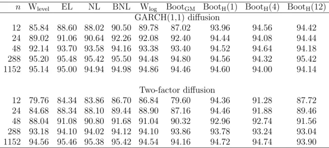
(µt, ρ1, ρ2) = (0,0,0)), we allow for drift and leverage effects by setting (µt, ρ1, ρ2) =
(0.0314,−0.576,0) for the GARCH(1,1) model, and (µt, ρ1, ρ2) = (0.030,−0.30,−0.30) for the two-factor diffusion model.
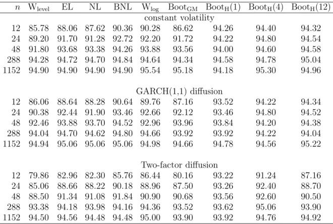
For these cases, we compare seven methods to construct two-sided 95% confidence intervals: (i) the Wald-type interval (Wlevel),2
(ii) the empirical likelihood (EL) in Theorem 2, (iii) the nonparametric likelihood (NL) with γ =−1 and φ =−1 + √35 in Theorem 7, (iv) the Bartlett corrected nonparametric likelihood (BNL) with the Bartlett correction factor 1 + 3/n in Theorem 8, (v) the logarithmic transform based Wald-type interval
(Wlog), (vi) the wild bootstrap based on the two-point distribution proposed in Gonçalves
and Meddahi (2009, Proposition 4.5) (BootGM), and (vii) the local gaussian bootstrap
proposed by Hounyo (2018) with block sizes M =1, 4, and 12. (BootH(M)). 3
Tables 1 and 2 present the actual coverage rates of each confidence interval across 10,000 Monte Carlo replications for five different sample sizes: n =1152, 288, 48, 24, and
12, which correspond to 1.25-minute, 5-minute, half-hour, 1-hour, and 2-hour returns, respectively. All methods tend to undercover, especially when the sample size n is small
2
The100(1−α)%asymptotic Wald -type confidence interval is
ˆ θ±zα/2 q ˆ V /n , whereVˆ = 23nPn i=1ri4. 3
(or sampling in a fixed time interval is not too frequent). However, we find that the performance of Hounyo’s (2018) local gaussian bootstrap is excellent. The two-factor model implies overall larger coverage distortions than the GARCH(1,1) model.
We first compare the proposed nonparametric likelihood methods (EL, NL, and BNL) and the conventional Wald confidence interval (Wlevel) to illustrate the discussions in
Section 2.3. Indeed, EL, NL, and BNL outperform Wlevel for all cases. Among these
nonparametric likelihood methods, BNL outperforms even for stochastic volatility models with drift and leverage effects despite the fact that the Bartlett correction in Theorem 8 does not theoretically provide an asymptotic refinement under non-constant volatility.
We now compare the nonparametric likelihood methods (EL, NL, and BNL) with the bootstrap methods (BootGM andBootH) and the logarithmic transform based Wald-type
interval (Wlog). For the GARCH(1,1) model,BootHby Hounyo (2018) tends to be closer to
the nominal level than the other methods, and our nonparametric likelihood methods show similar performance asBootGMby Gonçalves and Meddahi (2009) andWlog. For the
two-factor model, BNL, in particular, is favorably comparable withBootGM,BootH, and Wlog.
In this case, we should note that the results ofBootH may be sensitive to the choice of the
block size M. Overall, for the benchmark case, the proposed nonparametric likelihood
methods perform equally as well as Gonçalves and Meddahi’s (2009) wild bootstrap and the logarithmic transform based Wald interval, but less satisfactory than Hounyo’s (2018) local gaussian bootstrap. It is interesting to investigate whether Hounyo’s (2018) local approach can be adapted to our empirical likelihood approach (e.g., construct an empirical likelihood by exploiting the local Gaussian framework of Mykland and Zhang (2009)).
As discussed in Section 2.3, the nonparametric likelihood confidence intervals are range preserving while the conventional Wald-type confidence interval (Wlevel) may contain
of the Wald-type confidence intervals in Table 3. This shows that the Wald-type intervals tend to contain negative values particularly for small sample sizes.
5.2. Simulation 2: Test for jump. In this subsection we evaluate the finite sample properties of the nonparametric likelihood test for the presence of jumps discussed in Section 3.4. We adopt the simulation design in Dovonon et al. (2017), and consider the two-factor diffusion model with diurnality effects:
dlogSt = µtdt+σu,tσt(ρ1dW1t+ρ2dW2t+
q
1−ρ2
1−ρ22dW3t) +dJt,
σu,t = 0.88929198 + 0.75 exp(−10t) + 0.25 exp(−10(1−t)), σt=f(−1.2 + 0.04σ1t2 + 1.5σ2t2),
where dσ2
1t = −0.00137σ1t2dt+dW1t, dσ22t = −1.386σ22tdt + (1 + 0.25σ22t)dW2t, and f(·) is defined in (5.1). The process σu,t models the diurnal U-shaped pattern in intraday
volatility. When σu,t = 1 for t ∈ [0,1], the return process reduces to the simple case of no diurnality effects. Jt is a finite activity jump process modeled as a compound Poisson
process with constant jump intensity λ and random jump size distributed asN(0, σ2 jump). For the null hypothesis of no jump in the return process, we set σ2
jump = 0. For the alternative hypothesis, we set λ= 0.058 and σ2jump= 1.7241.
We compare four methods to test for jumps: (i) the Wald-type test (Wald),4
(ii) the (one-sided) empirical likelihood test (EL) presented after Theorem 6 using the tripower variation (m = 3 and p1 = p2 = p3 = 2/3), (iii) the adjusted Wald-type test by Huang
4
The Wald statistic is defined as Tn = √n(RVn −BVn)/pVnˆ , where RVn = Pn
i=1r2i, BVn = 1 µ2 1 Pn i=2|ri||ri−1|, andVnˆ = (µ−14+ 2µ− 2 1 −5)µ3n 4/3 Pn
i=3|ri|4/3|ri−1|4/3|ri−2|4/3. The test then rejects the
null of no jump at a significance level ofαwhenTn> z1−α, wherez1−α is the(1−α)-th quantile of the
and Tauchen (2005) (Waldadj),5
and (iv) the bootstrap test by Dovononet al. (2017) with L= 5 and M = 4 (Boot).6
We consider five different sample sizes: n=1152, 576, 288, 96, and 48, which correspond
to 1.25-minute, 2.5-minute, 5-minute, 15-minute, and half-hour returns. All results are based on 5,000 Monte Carlo replications.
Table 4 reports the rejection frequencies of the jump tests under the null of no jump at the 5% nominal significance level for both cases with and without diurnally effects. The Wald-type tests (both Wald and Waldadj) tend to over-reject for both cases especially
when the sample size is small (i.e., sampling in a fixed time interval is less frequent). In all cases, EL shows better performance in terms of the null rejection frequencies. The rejection frequencies vary from 9.3% (n = 1152) to 26.9% (n = 48) for Wald, from 7.4%
(n = 1152) to 17.2% (n = 48) for Waldadj, from 6.2% (n = 1152) to 10.7% (n = 48) for
Boot, while they vary from 5.3% (n= 1152) to 8.0% (n= 48) for EL.
We also analyze the power properties of the proposed jump test under the alternative hypothesis. We compare the calibrated powers of the four tests above (i.e., the rejection frequencies of these tests where the critical values are given by the Monte Carlo 95% percentiles of the corresponding test statistics under the data generation process satisfying the null hypothesis). Table 5 shows that EL is slightly less powerful than the other methods. Since EL has better null rejection properties than the others, these power properties characterize a tradeoff between the size and power properties of the empirical likelihood test and other tests.
5
The adjusted Wald-type statistic is defined as √ √n(1−BVn/RVn)
(µ−4 1 +2µ −2 1 −5) max{1,T Qn/BV 2 n} , where T Qn = n µ3 4/3 Pn i=3|ri|4/3|ri−1|4/3|ri−2|4/3. 6
The choice of L = 5 is based on the recommendation of Dovonon et al. (2017). The results are not very sensitive to the choice of M whenL= 5. In our simulations, the bootstrap test uses 499 bootstrap replications for each Monte Carlo replication.
5.3. Simulation 3: Noise robust inference. In Section B of the web appendix, we present additional simulation results for the noise robust empirical likelihood statistic discussed in Section 3.3.
6. Real data example
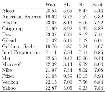
To mitigate microstructure noise, as suggested in Hansen and Lunde (2006) and Bandi and Russel (2008), we consider 5-minute data consisting of intra-day quotes of Alcoa,
American Express, Baxter, Citigroup, Dow, Gilead, Goldman Sachs, Intel Corporation, Met, Microsoft, Nike, Pfizer, Verizon and Yahoo from January 2, 2001 to November 15, 2005, which corresponds to 1236 trading days.
Table 6 reports the percentage of days identified with jumps for the period under investigation.7
To this end, we consider four methods to test for jumps: (i) the Wald-type test (Wald), (ii) (signed root) empirical likelihood (EL), (iii) (signed root) nonparametric likelihood (NL) with γ = −1 and φ = −1 + √35, and the bootstrap approach (Boot) proposed in Dovonon, Goncalves, Hounyo, and Meddahi (2018). In line with the Monte Carlo findings, we note that the Wald test tends to over detect jumps. Indeed, the percentage of days identified with jumps is always larger than 19%. EL, NL and Boot
imply very similar empirical findings. Using nonparametric likelihood procedures, the percentage of days identified with jumps is always smaller than 11%.
7. Conclusion
In this paper, we propose empirical likelihood-based methods for interval estimation and hypothesis testing of volatility measures using high frequency data. Our empirical likelihood approach is extended to be robust to the presence of jumps and microstructure 7
Our preliminary sensitivity analysis suggests that the results are qualitatively very similar for different sampling frequencies.
noise, and an empirical likelihood test to detect the presence of jumps is developed. We also investigate second-order properties of a general family of nonparametric likelihood statistics, and propose a method for Bartlett correction.
One important direction of future research is to extend our empirical likelihood ap-proach to develop a new point estimator under over-identified estimating equations, where the number of estimating equations exceeds the number of parameters. Over-identified estimating equations naturally emerge in the present context if we combine different esti-mating equations for the same object of interest. In this case, the resulting maximum em-pirical likelihood estimator can be different from the existing estimators, and is expected to be more efficient. This extension is currently under investigation by the authors.
Appendix A. Tables
n Wlevel EL NL BNL Wlog BootGM BootH(1) BootH(4) BootH(12) constant volatility 12 85.78 88.06 87.62 90.36 90.28 86.62 94.26 94.40 94.32 24 89.20 91.70 91.28 92.72 92.20 91.72 94.22 94.80 94.54 48 91.80 93.68 93.38 94.26 93.88 93.56 94.00 94.60 94.58 288 94.28 94.72 94.70 94.84 94.64 94.34 94.58 94.78 95.04 1152 94.90 94.90 94.90 94.90 95.54 95.18 94.18 95.30 94.96 GARCH(1,1) diffusion 12 86.06 88.64 88.28 90.64 89.76 87.16 93.52 94.22 94.34 24 90.38 92.44 91.90 93.46 92.66 92.12 93.46 94.80 94.52 48 92.46 93.88 93.70 94.52 92.96 93.96 93.84 94.20 94.38 288 94.04 94.70 94.62 94.80 94.66 93.92 93.92 94.22 94.04 1152 94.94 95.06 95.06 95.06 94.98 94.66 94.78 94.56 95.22 Two-factor diffusion 12 79.86 82.96 82.30 85.76 86.44 80.16 93.22 91.24 87.16 24 85.06 88.66 88.22 90.18 88.96 87.50 93.26 92.40 88.70 48 88.50 91.34 91.08 91.84 90.90 90.68 93.56 92.60 90.50 288 93.38 94.18 93.98 94.16 94.36 93.52 93.62 95.06 93.90 1152 94.50 94.56 94.48 94.48 95.00 93.90 93.92 94.76 94.92
Table 1. Coverage probabilities of nominal 95% confidence intervals for integrated volatility (no leverage and no drift case)
n Wlevel EL NL BNL Wlog BootGM BootH(1) BootH(4) BootH(12) GARCH(1,1) diffusion 12 85.84 88.60 88.02 90.50 89.78 87.02 93.96 94.56 94.42 24 89.02 91.06 90.64 92.26 92.08 92.40 94.44 94.08 94.44 48 92.14 93.70 93.58 94.16 93.38 93.40 94.52 94.64 94.18 288 95.20 95.48 95.42 95.50 94.48 94.80 94.56 94.32 95.42 1152 95.14 95.00 94.94 94.98 94.86 94.46 94.60 94.00 94.14 Two-factor diffusion 12 79.76 84.34 83.86 86.70 86.84 79.60 94.36 91.28 87.72 24 84.68 88.34 88.10 89.44 88.90 87.16 94.46 91.88 89.46 48 88.04 91.08 90.80 91.68 91.04 90.32 92.96 92.74 91.56 288 93.18 94.10 94.02 94.12 94.10 93.86 93.78 93.24 93.04 1152 94.56 95.46 95.38 95.42 94.54 94.16 94.72 94.74 93.90
Table 2. Coverage probabilities of nominal 95% confidence intervals for integrated volatility (with leverage and drift)
95% 99% 99.9% 95% 99% 99.9% n GARCH(1,1) diffusion Two-factor diffusion 12 80.64 99.85 100 91.86 99.96 100 24 6.94 43.60 95.44 40.61 79.32 99.02 48 0.01 0.47 7.21 8.75 25.59 58.14
288 0 0 0 0 0.04 0.23
1152 0 0 0 0 0 0
Table 3. Frequencies (measured by percentages) of negative left endpoints of 95%, 99%, and 99.9% Wald confidence intervals for integrated volatility (with leverage and drift)
n Wald EL Waldadj Boot Wald EL Waldadj Boot without diurnal effects with diurnal effects 48 22.4 8.0 14.6 8.5 26.9 7.3 17.2 10.7 96 15.1 5.7 9.9 7.3 18.8 5.4 13.3 8.9 288 11.2 4.9 8.3 6.2 12.0 4.9 9.6 7.4 576 10.4 5.7 8.3 6.4 11.7 5.7 9.7 7.1 1152 9.3 5.3 7.4 6.3 9.5 5.4 7.8 6.2
n Wald EL Waldadj Boot Wald EL Waldadj Boot without diurnal effects with diurnal effects 48 74.9 66.4 75.2 74.9 72.8 65.0 72.1 72.8 96 82.6 77.0 82.6 82.6 79.8 74.9 79.5 79.8 288 86.9 83.4 86.9 86.9 83.7 80.9 83.7 83.7 576 89.7 85.9 89.4 89.7 87.6 83.0 87.6 87.6 1152 89.7 85.9 89.4 89.7 87.6 84.5 87.6 87.6
Table 5. Calibrated power of jump tests
Wald EL NL Boot Alcoa 20.54 5.65 6.47 5.44 American Express 19.62 6.76 7.52 6.32 Baxter 23.67 8.13 8.76 7.22 Citigroup 21.69 8.92 9.37 8.88 Dow 23.07 7.76 8.12 7.11 Gilead 21.02 6.16 7.02 6.01 Goldman Sachs 19.76 4.87 5.24 4.67 Intel Corporation 21.11 7.34 7.61 6.85 Met 22.65 9.42 10.26 9.13 Microsoft 22.02 8.14 9.02 8.04 Nike 21.97 7.54 8.02 7.08 Pfizer 21.65 9.59 10.15 8.93 Verizon 22.15 7.06 7.56 6.84 Yahoo 22.87 8.05 9.23 7.84
Table 6. Percentage of days identified with jumps for the period from January 2, 2001 to November 15, 2005.
References
[1] Aït-Sahalia, Y. and J. Jacod (2009a) Testing for jumps in a discretely observed process, Annals of Statistics, 37, 184-222.
[2] Aït-Sahalia, Y. and J. Jacod (2009b) Estimating the degree of activity of jumps in high frequency data,Annals of Statistics, 37, 2202-2244.
[3] Aït-Sahalia, Y. and J. Jacod (2014) High-Frequency Financial Econometrics, Princeton University Press.
[4] Aït-Sahalia, Y., Mykland, P. A. and L. Zhang (2011) Ultra high frequency volatility estimation with dependent microstructure noise,Journal of Econometrics, 160, 160-175.
[5] Andersen, T. G., Dobrev, D. and E. Schaumburg (2012) Jump-robust volatility estimation using nearest neighbor truncation,Journal of Econometrics, 169, 75-93.
[6] Baggerly, K. A. (1998) Empirical likelihood as a goodness-of-fit measure,Biometrika, 85, 535-547. [7] Bandi, F. M. and J. R. Russell (2008) Microstructure noise, realized variance, and optimal sampling,
Review of Economic Studies, 75, 339-369.
[8] Barndorff-Nielsen, O. E., Graversen, S. E., Jacod, J. and N. Shephard (2006) Limit theorems for bipower variation in financial econometrics,Econometric Theory, 22, 677-719.
[9] Barndorff-Nielsen, O. E., Hansen, P. R., Lunde, A. and N. Shephard (2008) Designing realized kernels to measure the ex post variation of equity prices in the presence of noise,Econometrica, 76, 1481-1536.
[10] Barndorff-Nielsen, O. E. and N. Shephard (2002) Econometric analysis of realized volatility and its use in estimating stochastic volatility models,Journal of the Royal Statistical Society, B, 64, 253-280. [11] Barndorff-Nielsen, O. E. and N. Shephard (2004) Power and bipower variation with stochastic
volatil-ity and jumps,Journal of Financial Econometrics, 2, 1-37.
[12] Barndorff-Nielsen, O. E. and N. Shephard (2005). How accurate is the asymptotic approximation to the distribution of realised variance?, in Andrews, D. W. K. and J. H. Stock (eds.), Identification and Inference for Econometric Models, Cambridge University Press, 306-331.
[13] Barndorff-Nielsen, O. E. and N. Shephard (2006) Econometrics of testing for jumps in financial economics using bipower variation,Journal of Financial Econometrics, 4, 1-30.
[14] Barndorff-Nielsen, O. E., Shephard, N. and M. Winkel (2006) Limit theorems for multipower varia-tion in the presence of jumps,Stochastic Processes and their Applications, 116, 796-806.
[15] Choi, S., Hall, W. J. and A. Schick (1996) Asymptotically uniformly most powerful tests in parametric and semiparametric models,Annals of Statistics, 24, 841-861.
[16] Cressie, N. and T. R. C. Read (1984) Multinomial goodness-of-fit tests,Journal of the Royal Statis-tical Society, B, 46, 440-464.
[17] DiCiccio, T. J., Hall, P. and J. Romano (1991) Empirical likelihood is Bartlett-correctable, Annals of Statistics, 19, 1053-1061.
[18] Dumitru, A.-M. and G. Urga (2012) Identifying jumps in financial assets: A comparison between nonparametric jump tests,Journal Business & Economic Statistics, 30, 242-255.
[19] Dovonon, P., Gonçalves, S. and N. Meddahi (2013) Bootstrapping realized multivariate volatility measures,Journal of Econometrics, 172, 49-65.
[20] Dovonon, P., Gonçalves, S., Hounyo, U. and N. Meddahi (2017) Bootstrapping high-frequency jump tests, forthcoming inJournal of the American Statistical Association.
[21] Gonçalves, S. and N. Meddahi (2008) Edgeworth corrections for realized volatility, Econometric Reviews, 27, 139-162.
[22] Gonçalves, S. and N. Meddahi (2009) Bootstrapping realized volatility,Econometrica, 77, 283-306. [23] Gonçalves, S. and N. Meddahi (2011). Box-Cox transforms for realized volatility,Journal of
Econo-metrics, 160, 129-144.
[24] Hansen, P. R. and A. Lunde (2006), Realized variance and market microstructure noise,Journal of Business & Economic Statistics, 24, 127-161.
[25] Hall, P. and B. La Scala (1990) Methodology and algorithms of empirical likelihood, International Statistical Review, 58, 109-127.
[26] Heston, S. L. (1993) A closed-form solution for options with stochastic volatility with applications to bond and currency options,Review of Financial Studies, 6, 327-343.
[27] Hjort, N. L., McKeague, I. W. and I. van Keilegom (2009) Extending the scope of empirical likelihood,
Annals of Statistics, 37, 1079-1111.
[28] Hounyo, U. (2018) A local Gaussian bootstrap method for realized volatility and related beta, forth-coming inEconometric Theory.
[29] Hounyo, U., Gonçalves, S. and N. Meddahi (2017) Bootstrapping pre-averaged realized volatility under market microstructure noise,Econometric Theory, 33, 791-838.
[30] Hounyo, U. and B. Veliyev (2016) Validity of Edgeworth expansions for realized volatility estimators,
Econometrics Journal, 19, 1-32.
[31] Huang, X. and G. Tauchen (2005) The relative contribution of jumps to total price variance,Journal of Financial Econometrics, 3, 456-499.
[32] Jacod, J., Li, Y., Mykland, P. A., Podolskij, M. and M. Vetter (2009) Microstructure noise in the continuous case: the pre-averaging approach, Stochastic Processes and their Applications, 119, 2249-2276.
[33] Jacod, J. and P. Protter (1998) Asymptotic error distributions for the Euler method for stochastic differential equations,Annals of Probability, 26, 267-307.
[34] Jacod, J. and M. Rosenbaum (2013) Quarticity and other functionals of volatility: Efficient estima-tion,Annals of Statistics, 41, 1462-1484.
[35] Kong, X.-B. (2012) Confidence interval of the jump activity index based on empirical likelihood using high frequency data,Journal of Statistical Planning and Inference, 142, 1378-1387.
[36] Kitamura, Y. (1997) Empirical likelihood methods with weakly dependent process, Annals of Sta-tistics, 25, 2084-2102.
[37] Li, Y., Zhang, Z. and X. Zheng (2013) Volatility inference in the presence of both endogenous time and microstructure noise,Stochastic Processes and their Applications, 123, 2696-2727.
[38] Mykland, P. A. and L. Zhang (2009) Inference for continuous semimartingales observed at high frequency,Econometrica, 77, 1403-1445.
[39] Owen, A. B. (1988) Empirical likelihood ratio confidence intervals for a single functional,Biometrika, 75, 237-249.
[40] Owen, A. B. (2001) Empirical Likelihood, Chapman and Hall/CRC.
[41] Podolskij, M. and N. Yoshida (2016) Edgeworth expansion for functionals of continuous diffusion processes,Annals of Applied Probability, 26, 3415-3455.
[42] Renault, E., Sarisoy, C. and B. J. M. Werker (2017) Efficient estimation of integrated volatility and related processes,Econometric Theory, 33, 439-478.
[43] Schennach, S. M. (2005) Bayesian exponentially tilted empirical likelihood,Biometrika, 92, 31-46. [44] Schennach, S. M. (2007) Point estimation with exponentially tilted empirical likelihood, Annals of
Statistics, 35, 634-672.
[45] Zhang, L., Mykland, P. A. and Y. Aït-Sahalia (2005) A tale of two time scales: determining integrated volatility with noisy high-frequency data,Journal of the American Statistical Association, 100, 1394-1411.
[46] Zhang, L., Mykland, P. A. and Y. Aït-Sahalia (2011) Edgeworth expansions for realized volatility and related estimators,Journal of Econometrics, 160, 190-203
University of Applied Sciences and Arts of Italian Switzerland, Galleria 2 - 100 Via Cantonale 6928, Manno, CH
E-mail address: [email protected]
Graduate School of Economics, Hitotsubashi University, 2-1 Naka, Kunitachi, Tokyo 186-8601, Japan.
E-mail address: [email protected]
Department of Economics, London School of Economics, Houghton Street, London, WC2A 2AE, UK.