SFB 649 Discussion Paper 2005-022
DSFM fitting of Implied
Volatility Surfaces
Szymon Borak*
Matthias R. Fengler*
Wolfgang Härdle*
* CASE – Center for Applied Statistics and Economics, Humboldt-Universität zu Berlin, Germany
This research was supported by the Deutsche
Forschungsgemeinschaft through the SFB 649 "Economic Risk". http://sfb649.wiwi.hu-berlin.de
ISSN 1860-5664
SFB 649, Humboldt-Universität zu Berlin Spandauer Straße 1, D-10178 Berlin
S
FB
6
4
9
E
C
O
N
O
M
I
C
R
I
S
K
B
E
R
L
I
N
DSFM fitting of Implied Volatility Surfaces
Szymon Borak, Matthias Fengler and Wolfgang H¨ardle
CASE - Center for Applied Statistics and Economics
Humboldt-Universit¨at zu Berlin
Spandauer Straße 1, 10178 Berlin, Germany
borak@wiwi.hu-berlin.de
Abstract
Implied volatility is one of the key issues in modern quan-titative finance, since plain vanilla option prices contain vi-tal information for pricing and hedging of exotic and illiq-uid options. European plain vanilla options are nowadays widely traded, which results in a great amount of high-dimensional data especially on an intra day level. The data reveal a degenerated string structure. Dynamic Semipara-metric Factor Models (DSFM) are tailored to handle com-plex, degenerated data and yield low dimensional represen-tations of the implied volatility surface (IVS). We discuss estimation issues of the model and apply it to DAX option prices.
JEL classification codes:C14
1. Introduction
The Black-Scholes formula (BS) for calculating the price of a European plain vanilla option is one of the most rec-ognized results in modern quantitative finance. The price is given as a function of the price of the underlying, a strike price, the interest rate, time to maturity and an unobserved volatility. By plugging the observed option price into the BS formula it is straightforward to calculate the implied volatil-ity (IV). The surface (on dayt) given by the mapping from moneynessκ(a measure of strikes) and from time to ma-turityτ (κ, τ) → bσt(κ, τ)is called implied volatility sur-face (IVS). The observed IVS, Figure 1, reveals a non-flat profile across moneyness (called “smile” or “smirk”) and across time to maturity.
Despite the deficiencies of the BS model it is popular among practitioners to quote option prices in terms of IV due to its intuitive simplicity. However there were many efforts to model a non constant IVS. One possible approach is to change the dynamics of the process of the underlying as-set by increasing its degree of freedom. This leads to
para-metric models with jumps like in [14], stochastic volatil-ity like in [13] and [12] or models based on L´evy processes like the generalized hyperbolic in [4] among many others. The models reproduce the smile phenomenon and their pa-rameters are calibrated from the option prices by minimiz-ing cost functional. One may also consider local volatility (LV) models like in [3] where the volatility is assumed to be a function of time and the price of the underlying. There ex-ist an analytical formula which allows to calibrate this sur-face (LVS) straightforward from the IVS.
A drawback even of the most sophisticated models is the failure to correctly describe the dynamics of the IVS. This can be inferred from frequent recalibration of the model and has been best understood in the context of LV-models [10]. Consequently, studying the IVS as an additional market fac-tor has become a vital stand of research. The main focus is on a low dimensional approximation of the IVS based on principal components analysis (PCA). The PCA is applied both to the term structure of the IVS ([16] or [7]) and strike dimension (eg. [15]). The common PCA for several matu-rity groups is studied in [8] and the functional PCA was dis-cussed in [1] and [2].
Our approach is to represent the IVS as the sum of factors treated as two dimensional functions depending on money-ness and maturity. In [2] the factors are obtained using the functional PCA for the IVS fitted on a grid for each partic-ular day. However this fit may be biased due to the degener-ated data design. In [9] the IVS is obtained as a projection on parametric factors which has to be initially specified. In DSFM the factors are estimated from the data, which al-lows flexible modelling. Contrary to [2] the IVS is obtained as a fit to the factors smoothed in time, which reflects the dynamics of the whole system.
The paper is organized as follows: in the next section we de-scribe the DSFM and present the estimation procedure. In Section 3 we discuss the estimation issues and proposed im-provements of the algorithm. Section 4 presents the empir-ical results on DAX options and discusses briefly possible applications.
2. DSFM
IVS Ticks 20000502 Data Design
0.4 0.5 0.6 0.70.8 0.9 1 1.1 1.21.3 1.4 Moneyness 0 0.1 0.2 0.3 0.4 0.5 0.6 0.7 Time to maturity
Figure 1. Left panel: implied volatilities ob-served on 2nd May, 2000. Right panel: data design on 2nd May, 2000.
Institutional conventions of the option market entail a spe-cific degenerated IV data design. Each day one observes only a small number of maturities which form typi-cal ‘strings’. The usual data pattern is visible in the right panel of Figure 1. Options belonging to the same string have a common time to maturity but different money-ness. In the left panel of the Figure 1 IV smiles are pre-sented. One can easily see different curvatures for a each time to maturity. As time passes not only do the strings move through the space towards expiry but they also change their shape and level randomly.
In order to capture this complex dynamic structure of the IVS a DSFM was proposed in [6]. It offers a low-dimensional representation of the IVS, which is ap-proximated by basis functions in a finite dimensional func-tion space. The basis funcfunc-tions are unknown and have to be estimated from the data. The IVS dynamics are ex-plained by loading coefficients, which form a multidimen-sional time series.
LetYi,j be the log-implied volatility observed on a
partic-ular day. The indexi is the number of the day, while the total number of days is denoted byI(i= 1, ..., I). The in-dexj represents an intra-day trade on dayiand the num-ber of trades on that day isJi (j = 1, ...Ji). LetXi,j be
a two-dimensional variable containing moneynessκi,j and
maturityτi,j. Among many moneyness settings we define
it asκi,j = Ki,j
Fti , whereKi,jis a strike andFti the
under-lying futures price at timeti. The DSFM regressesYi,jon
Xi,jby: Yi,j=m0(Xi,j) + L X l=1 βi,lml(Xi,j), (1)
wherem0is an invariant basis function,ml(l= 1, ...L) are
the ‘dynamic’ basis functions andβi,lare the factor weights
depending on timei.
2.1. Estimation
The estimatesβbi,landmblare obtained by minimizing the following least squares criterion (βi,0= 1):
I X i=1 Ji X j=1 Z ( Yi,j− L X l=0 b βi,lmbl(u) )2 Kh(u−Xi,j)du, (2) where Kh denotes a two-dimension kernel
func-tion. The possible choice for two-dimensional kernels is a product of one dimensional kernels
Kh(u) = kh1(u1) × kh2(u2), where h = (h1, h2)
>
are bandwidths andkh(v) = k(h−1v)/his a one dimen-sional kernel function.
The minimization procedure searches through all functions b
ml:R2−→R(l = 0, ..., L) and time seriesβbi,l∈R(i=
1, ..., I;l= 1, ..., L).
To calculate the estimates an iterative procedure is applied. First we introduce the following notation for1≤i≤I:
b pi(u) = 1 Ji Ji X j=1 Kh(u−Xi,j), (3) b qi(u) = 1 Ji Ji X j=1 Kh(u−Xi,j)Yi,j. (4) We denote bymb(r)= ( b
m(0r), ...,mb(Lr))>the estimate of the basis functions andβb
(r)
i = (βb
(r)
i,l, ...,βb
(r)
i,L)>the factor
load-ings on the dayiafterriterations. By replacing each func-tionmblin (2) bymbl+δgwith arbitrary functiongand tak-ing derivatives with respect toδone obtains:
I X i=1 Ji X j=1 ( Yi,j− L X l=0 b βi,lmbl(Xi,j) ) b βi,l0Kh(u−Xi,j) = 0. (5) Rearranging terms in (5) and plugging in (3)-(4) yields:
I X i=1 Jiβbi,l0 b qi(u) = I X i=1 Ji L X l=0 b βi,l0βbi,lpbi(u)mbl(u), (6)
for0≤l0≤L. In fact (6) is a set ofL+ 1equations. Define the matrixB(r)(u)and vectorQ(r)(u)by their elements:
B(r)(u) l,l0 = I X i=1 Jiβb (r−1) i,l0 βb (r−1) i,l pbi(u), (7)
Q(r)(u) l = I X i=1 Jiβb (r−1) i,l bqi(u). (8)
Thus (6) is equivalent to:
B(r)(u)mb(r)(u) =Q(r)(u) (9)
which yields the estimate ofmb(r)(u)in ther-th iteration. A similar idea has to be applied to updateβb
(r)
i . Replacing
b
βi,lbyβbi,l+δin (2) and taking once more the derivative
with respect toδyields:
Ji X j=1 Z Yi,j− L X l=0 b βi,lmbl(Xi,j) b ml0(u)Kh(u−Xi,j)du= 0, (10)
which leads to:
Z b qi(u)mbl0(u)du= L X l=0 b βi,l Z b pi(u)mbl0(u) b ml(u)du, (11) for1≤l0 ≤L. The formula (11) is now a system ofL equa-tions. Define the matrixM(r)(i)and the vectorS(r)(i)by their elements: M(r)(i)l,l0 = Z b pi(u)mbl0(u) b ml(u)du, (12) S(r)(i) l= Z b qi(u)mbl(u)du− Z b pi(u)mb0(u)mbl(u)du. (13) An estimate ofβb (r)
i is thus given by solving:
M(r)(i)βb
(r)
i =S
(r)(i). (14)
The algorithm stops when only minor changes occur:
I X i=1 Z L X l=0 b βi,l(r)mbl(r)(u)−βb (r−1) i,l mb (r−1) l (u) !2 du≤ (15) for some small. Obviously one needs to set initial values ofβb
(0)
i in order to start the algorithm.
2.2. Orthogonalization and normalization
The estimates mb = (mb1, ...,mbL)
> of the basis
func-tions are not uniquely defined. They can be replaced by functions that span the same affine space. Define bp(u) =
1
I
PI
i=1pbi(u)and theL×LmatrixΓby its elements
Γl,l0 = Z b ml(u)mbl0(u) b p(u)du.
The estimates mb are replaced by new functionsmbnew = (mbnew1 , ...,mb new L )>: b mnew0 = mb0−γ>Γ−1mb b mnew = Γ−1/2mb
such that they are now orthogonal in theL2( b
p)space. The loading time series estimatesβbi = (βbi,1, ...,βbi,L)>need to be substituted by:
b
βinew= Γ−1/2(βbi+ Γ−1γ) (16)
whereγis (L×1) vector withγl=
R b
m0(u)mbl(u)pb(u)du. The next step is to choose an orthogonal basis such that for eachw = 1, ..., Lthe explanation achieved by the partial sum: m0(u) + w X l=1 βi,lml(u)
is maximal. One proceeds as in PCA. First define a ma-trixB with Bl,l0 = PI
i=1βbi,lβbi,l0 and Z = (z1, ..., zL)
wherez1,...,zL are the eigenvectors ofB. Then replacemb bymbnew=Z>
b
mandβbibyβbinew=Z>βbi.
The orthonormal basis mb1, ...,mbL is chosen such that PI
i=1βb2i,1 is maximal and given βbi,1,mb0,mb1 the quan-tityPI
i=1βbi,22is maximal and so forth.
3. Estimation issues
The estimation procedure encounter several computational challenges. The basis factor functions can be represented on the finite grid only, which obviously may not cover the whole desired estimation space. One also needs to choose some kernel function, the bandwidths and the initial load-ing time seriesβb
(0)
i . Due to the degenerated design of the
IV data proper decision of these points is a key issue in suc-cessful model estimation.
3.1. Implementation
As a numerical result of the estimationLtime series (βbi,l)
andL+ 1functions (mbl) given on the finite grid are
ob-tained. The choice of the grid needs to be arbitrary and depends on the density of the data points. The data (Xi,j
and Yi,j) comes into the computation only in bpi(u) and
b
qi(u), which has to be calculated before the main itera-tion procedure. The calculaitera-tion of pbi(u)and bqi(u), how-ever, is the main computation effort in the estimation proce-dure. Therefore we believe that the DSFM can be used ef-ficiently in a ’sliding window’ type of analysis. Updating ofpbi(u)andqbi(u)requires calculations only for one addi-tional day, which is not a big computaaddi-tional issue.
3.2. Bandwidths dependence
In derivative market one can observe fairly many different types of option contracts. Each day one may trade options with several different time to maturities and many differ-ent strikes. However the number of possible strikes is much higher than the number of maturities, which results in the string structure. Moreover the contracts with smaller ma-turities are traded more intensively and there tend to exist more contracts for the smaller time to maturities for which the difference between two successive expiry days is one month (1M, 2M, 3M), but for the next maturity range it in-creases to three months (6M, 9M, 12M).
Since the strings are moving in the maturity vs. moneyness plane towards expiry one needs to pool many days in order to fill the plane with observations. However due to an un-equal distribution of data points one needs even more days to fill the range with bigger maturities than with smaller ones. Otherwise one faces gaps for some particular matu-rity range.
These gaps may obstruct the estimation procedure. If in any pointu0the functionpb(u0) = 0in (3) then obviously matrix
B(r)(u0)in (7) contains only0and is singular. This means
that one may not estimate successfully any value of the IVS in this point.
This problem may be solved by increasing the bandwidths but it may lead also to a larger bias. One may also use a ker-nel function with infinite support like the Gaussian kerker-nel but instead of analytical zeros numerical zeros creep in. An-other possibility is to use the k-nearest neighbor estimator. In the range with many data, however, one takes into consid-eration only very few observations closest to the grid points. On the other hand in the range with few points the estima-tor is based on the observations far from the grid points. In order to cope with the degenerated data design local band-widths can be applied. In (3) and (4) the fixed bandband-widths are replaced by bandwidths dependent on time to maturity and moneyness: b pi(u) = 1 Ji Ji X j=1 Kh(u)(u−Xi,j), (17) b qi(u) = 1 Ji Ji X j=1 Kh(u)(u−Xi,j)Yi,j. (18)
Due to the described data design we propose to keep the bandwidths in the moneyness direction constant and lin-early increasing in the maturity dimension. For the optimal choice of the bandwidths we refer to [11].
3.3. Initial parameter dependence
The problem of gaps in the data cannot only be handled with the size of the bandwidths. Of course it is obligatory thatbpi(u)needs to be non-zero for at least onei. However this is not a sufficient condition to ensure non singularity of the matrixB(r)(u0). The initial estimates of
b
βi(0)play also an important role.
In [6] a piecewise constant initial time series was proposed. The subintervalsI1, ..., IL are pairwise disjoint subsets of {1, ..., I} andSL
l=1Il is a strict subset of {1, ..., I}. The initial estimates are now defined byβb
(0)
i,l = 1ifi∈Iland
b
βi,l(0) = 0ifi /∈ Il. To complete the settingβb (0)
i,0 = 1for
eachi.
However this kind of setting requires even more data to ob-tain the final estimates. For each subsetIlthere needs to
ex-ist at least one dayisuch thatpbi(u0)6= 0, otherwise the row of zeros in (7) appears. The smaller is the length ofIl
in-tervals the bigger bandwidths need to be taken. This defi-ciency can be removed by taking a random initial time se-ries.
4. Results
For our analysis we employ tick statistics on DAX index op-tions from January 1999 to February 2003. By inverting the BS formula one easily obtains IV. We regard as outliers ob-servations with IV bigger that0.8 and smaller than0.04. We also remove observations with maturity less than10day since their behavior in this range is irregular due to expiry effect.
We apply the algorithm on an equidistant grid covering moneynessκ∈[0.8,1.2]and time to maturity measured in yearsτ∈[0.05,1.00]. In each direction our grid consists of
25points. We set the number of dynamic basis functions to
L= 3like in [6]. In the moneyness direction we apply con-stant bandwidthsh1 = 0.03and in order to get smoother estimates of the basis functions in the maturity direction we use linearly increasing bandwidths. On the smallest ma-turity grid points we set bandwidths on0.02 and increase them linearly to0.2for the greatest maturity points. As the starting values ofβb(0) we take a piecewise constant series on disjoint time intervals. The initial weights selection is discussed below.
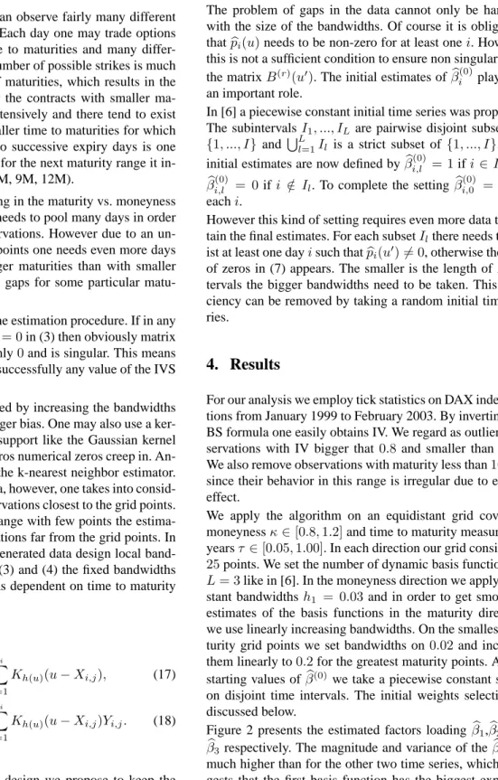
Figure 2 presents the estimated factors loadingβb1,βb2 and b
β3 respectively. The magnitude and variance of theβb1are much higher than for the other two time series, which sug-gests that the first basis function has the biggest explana-tory power of the IVS variation. This is actually not surpris-ing since the basis functions were ordered with respect to the biggest variance of loading factors.
1999 2000 2001 2002 2003 X 0 0.5 1 1.5 Y beta1 beta2 beta3
Figure 2. Time series of weightsβb1,βb2andβb3.
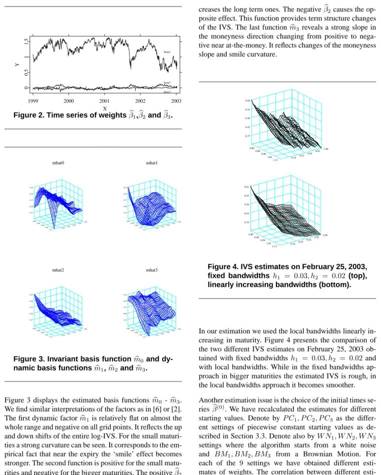
mhat0 0.24 0.43 0.62 0.81 1.00 0.80 0.88 0.96 1.04 1.12 -0.37 -0.26 -0.15 -0.04 0.07 mhat1 0.24 0.43 0.62 0.81 1.00 0.80 0.88 0.96 1.04 1.12 -1.02 -0.88 -0.73 -0.58 -0.43 mhat2 0.24 0.43 0.62 0.81 1.00 0.80 0.88 0.96 1.04 1.12 -0.37 -0.26 -0.15 -0.04 0.07 mhat3 0.24 0.43 0.62 0.81 1.00 0.80 0.88 0.96 1.04 1.12 -1.02 -0.88 -0.73 -0.58 -0.43
Figure 3. Invariant basis functionmb0 and
dy-namic basis functionsmb1,mb2andmb3.
Figure 3 displays the estimated basis functionsmb0 - mb3. We find similar interpretations of the factors as in [6] or [2]. The first dynamic factormb1is relatively flat on almost the whole range and negative on all grid points. It reflects the up and down shifts of the entire log-IVS. For the small maturi-ties a strong curvature can be seen. It corresponds to the em-pirical fact that near the expiry the ‘smile’ effect becomes stronger. The second function is positive for the small matu-rities and negative for the bigger matumatu-rities. The positiveβb2 increases short term maturities IVs and simultaneously
de-creases the long term ones. The negativeβb2causes the op-posite effect. This function provides term structure changes of the IVS. The last functionmb3 reveals a strong slope in the moneyness direction changing from positive to nega-tive near at-the-money. It reflects changes of the moneyness slope and smile curvature.
0.24 0.43 0.62 0.81 1.00 0.80 0.88 0.96 1.04 1.12 0.37 0.42 0.48 0.54 0.60 0.24 0.43 0.62 0.81 1.00 0.80 0.88 0.96 1.04 1.12 0.39 0.44 0.50 0.55 0.61
Figure 4. IVS estimates on February 25, 2003, fixed bandwidths h1 = 0.03, h2 = 0.02 (top),
linearly increasing bandwidths (bottom).
In our estimation we used the local bandwidths linearly in-creasing in maturity. Figure 4 presents the comparison of the two different IVS estimates on February 25, 2003 ob-tained with fixed bandwidths h1 = 0.03, h2 = 0.02 and with local bandwidths. While in the fixed bandwidths ap-proach in bigger maturities the estimated IVS is rough, in the local bandwidths approach it becomes smoother. Another estimation issue is the choice of the initial times se-riesβb(0). We have recalculated the estimates for different starting values. Denote by P C1, P C2, P C3 as the differ-ent settings of piecewise constant starting values as de-scribed in Section 3.3. Denote also byW N1, W N2, W N3 settings where the algorithm starts from a white noise and BM1, BM2, BM3 from a Brownian Motion. For each of the 9 settings we have obtained different mates of weights. The correlation between different esti-mates ofβb1,βb2andβb3are respectively:
1.0 −1.0 −1.0 −1.0 −1.0 1.0 −0.9 0.9 −0.9 1.0 1.0 1.0 1.0 −1.0 0.9 −0.9 0.9 1.0 1.0 1.0 −1.0 0.9 −0.9 0.9 1.0 1.0 −1.0 0.9 −0.9 0.9 1.0 −1.0 0.9 −0.9 0.9 1.0 −0.9 0.9 0.9 1.0 −1.0 1.0 1.0 −1.0 1.0 1.0 1.0 1.0 −1.0 −1.0 −1.0 0.3 −0.3 −0.3 1.0 1.0 −1.0 −1.0 −1.0 0.3 −0.3 −0.3 1.0 −1.0 −1.0 −1.0 0.3 −0.3 −0.3 1.0 1.0 1.0 −0.3 0.3 0.3 1.0 1.0 0.3 0.3 0.3 1.0 −0.3 0.3 0.3 1.0 −1.0 −1.0 1.0 1.0 1.0 1.0 −1.0 −1.0 −1.0 −1.0 1.0 −0.8 0.8 −0.8 1.0 1.0 1.0 −1.0 1.0 0.8 −0.8 0.8 1.0 1.0 −1.0 1.0 0.8 −0.8 0.8 1.0 −1.0 1.0 0.8 −0.8 0.8 1.0 −1.0 −0.8 0.8 −0.8 1.0 0.8 −0.8 0.8 1.0 −1.0 1.0 1.0 −1.0 1.0
where the sequence of the settings is following:
P C1, P C2, P C3, W N1, BM1, BM2, W N2, W N3, BM3. The algorithm converges to two different solutions depend-ing on the startdepend-ing values since the settdepend-ings form clearly two clusters: (P C1, P C2, P C3, W N1, BM1, BM2) and (W N2, W N3, BM3). Inside the clusters the weights are al-most perfectly correlated - top left and bottom right corners of the matrices contain1 or−1. Of course if the correla-tion of the time series estimates is−1the same factors are considered because they are identifiable only up to sign. Be-tween the clusters the correlation is not so strong. In or-der to choose one solution other criteria like explained variance or smoothness of IVS need to be taken into ac-count.
The DSFM can easily be applied in hedging or risk manage-ment. Computing sensitivity with respect to factor loadings changes simplify the vega hedge since the whole dynamics of the IVS is reduced toLfactors. After estimating stochas-tic model forβb, like in [5] where VAR(2) was detected, it can be used for scenario generation in Monte Carlo frame-work. Therefore it allows to compute the VaR for portfolios containing options.
5. Conclusion
We discuss estimation issues of the DSFM, which gives a flexible way of handling IV data and is a convenient mod-elling tool. We study the dependence on the startingβband the bandwidths settings. These are the key issues in effi-cient application of the model, which is left for future re-search.
6. Acknowledgement
We gratefully acknowledge financial support by the Deutsche Forschungsgemeinschaft and the Sonder-forschungsbereich 649 “ ¨Okonomisches Risiko”.
References
[1] M. Benko and W. H¨ardle. Common Functional Implied Volatility Analysis in P. ˇC´ıˇzek, W. H¨ardle and R. Weron (eds) Statistical Tools for Fianance and Insurance, chap-ter 5, pages 115–134. Springer Verlag, 2005.
[2] R. Cont and J. da Fosenca. Dynamics of implied volatility surfaces. Quantitative Finance, 2:45–60, February 2002. [3] B. Dupire. Pricing with a smile. RISK, 1(7):18–20, 1994. [4] E. Eberlein and K. Prause. The generalized hyperbolic
model: Financial derivatives and risk measures in H.
Ger-man, D. Madan, S. Pliska, T. Vorst (eds) Mathematical
Fi-nance - Bachelier Congress 2000 pages 245–267. Springer
Verlag, 2002.
[5] M. Fengler. Semiparametric Modelling of Implied Volatility. PhD thesis, Humboldt-Universit¨at zu Berlin, 2004.
[6] M. Fengler, W. H¨ardle, and E. Mammen. A Dynamic Semi-parametric Factor Model for Implied Volatility String Dy-namics. CASE Discussion Paper, Humboldt-Universit¨at zu Berlin, 2004.
[7] M. Fengler, W. H¨ardle, and P. Schmidt. Common factors govering VDAX movements and the maximum loss. Journal
of Financial Markets and Portfolio Managment, 1(16):16–
19, 2002.
[8] M. Fengler, W. H¨ardle, and C. Villa. The Dynamics of Implied Volatilities: A Common Principal Components Ap-proach. Review of Derivatives Research, 6:179–202, 2003. [9] R. Hafner. Stochastic Implied Volatility. Springer-Verlag,
Berlin Heidelberg, 2004.
[10] P. Hagan, D. Kumar, D. Lesniewski and D. Woodward. Manging smile risk. Wilmott magazine, 1:84–108, 2002. [11] W. H¨ardle. Applied Nonparametric Regression. Cambridge
University Press,1990.
[12] S. Heston. A closed-form solution for options with stochas-tic volatility with applications to bond and currency options.
Review of Financial Studies, 6:327–343, 1993.
[13] J. Hull, A. White The pricing on option on assets with stochastic volatilities. Journal of Finance, 42:281–300,
1987.
[14] R. Merton. Option pricing when underlying stock returns are discontinuous. Journal of Financial Economics, 3:125–144, 1976.
[15] G. Skiadopoulos, S. Hodges, and L. Clewlow. The dynamics of the S&P 500 implied volatility surface. Review of
Deriva-tives Research, 3:263–282, 1999.
[16] Y. Zhu and M. Avellaneda. An E-ARCH model for the term-structure of implied volatility of FX options. Applied
SFB 649 Discussion Paper Series
For a complete list of Discussion Papers published by the SFB 649,
please visit http://sfb649.wiwi.hu-berlin.de.
001 "Nonparametric Risk Management with Generalized
Hyperbolic Distributions" by Ying Chen, Wolfgang Härdle
and Seok-Oh Jeong, January 2005.
002 "Selecting Comparables for the Valuation of the European
Firms" by Ingolf Dittmann and Christian Weiner, February
2005.
003 "Competitive Risk Sharing Contracts with One-sided
Commitment" by Dirk Krueger and Harald Uhlig, February
2005.
004 "Value-at-Risk Calculations with Time Varying Copulae" by
Enzo Giacomini and Wolfgang Härdle, February 2005.
005 "An Optimal Stopping Problem in a Diffusion-type Model with
Delay" by Pavel V. Gapeev and Markus Reiß, February 2005.
006 "Conditional and Dynamic Convex Risk Measures" by Kai
Detlefsen and Giacomo Scandolo, February 2005.
007 "Implied Trinomial Trees" by Pavel Čížek and Karel
Komorád, February 2005.
008 "Stable Distributions" by Szymon Borak, Wolfgang Härdle
and Rafal Weron, February 2005.
009 "Predicting Bankruptcy with Support Vector Machines" by
Wolfgang Härdle, Rouslan A. Moro and Dorothea Schäfer,
February 2005.
010 "Working with the XQC" by Wolfgang Härdle and Heiko
Lehmann, February 2005.
011 "FFT Based Option Pricing" by Szymon Borak, Kai Detlefsen
and Wolfgang Härdle, February 2005.
012 "Common Functional Implied Volatility Analysis" by Michal
Benko and Wolfgang Härdle, February 2005.
013 "Nonparametric Productivity Analysis" by Wolfgang Härdle
and Seok-Oh Jeong, March 2005.
014 "Are Eastern European Countries Catching Up? Time Series
Evidence for Czech Republic, Hungary, and Poland" by Ralf
Brüggemann and Carsten Trenkler, March 2005.
015 "Robust Estimation of Dimension Reduction Space" by Pavel
Čížek and Wolfgang Härdle, March 2005.
016 "Common Functional Component Modelling" by Alois Kneip
and Michal Benko, March 2005.
017 "A Two State Model for Noise-induced Resonance in Bistable
Systems with Delay" by Markus Fischer and Peter Imkeller,
March 2005.
SFB 649, Spandauer Straße 1, D-10178 Berlin http://sfb649.wiwi.hu-berlin.de
This research was supported by the Deutsche
018 "Yxilon – a Modular Open-source Statistical Programming
Language" by Sigbert Klinke, Uwe Ziegenhagen and Yuval
Guri, March 2005.
019 "Arbitrage-free Smoothing of the Implied Volatility Surface"
by Matthias R. Fengler, March 2005.
020 "A Dynamic Semiparametric Factor Model for Implied
Volatility String Dynamics" by Matthias R. Fengler, Wolfgang
Härdle and Enno Mammen, March 2005.
021 "Dynamics of State Price Densities" by Wolfgang Härdle and
Zdeněk Hlávka, March 2005.
022 "DSFM fitting of Implied Volatility Surfaces" by Szymon
Borak, Matthias R. Fengler and Wolfgang Härdle, March
2005.
SFB 649, Spandauer Straße 1, D-10178 Berlin http://sfb649.wiwi.hu-berlin.de
This research was supported by the Deutsche