A Regularized, Model-Based Approach to Phase-Based
Conductivity Mapping Using MRI
Kathleen M. Ropella* and Douglas C. Noll
Purpose: To develop a novel regularized, model-based approach to phase-based conductivity mapping that uses structural information to improve the accuracy of conductivity maps.Theory and Methods: The inverse of the three-dimensional Laplacian operator is used to model the relationship between measured phase maps and the object conductivity in a penal-ized weighted least-squares optimization problem. Spatial masks based on structural information are incorporated into the problem to preserve data near boundaries. The proposed Inverse Laplacian method was compared against a restricted Gaussian filter in simulation, phantom, and human experiments.
Results: The Inverse Laplacian method resulted in lower reconstruction bias and error due to noise in simulations than the Gaussian filter. The Inverse Laplacian method also pro-duced conductivity maps closer to the measured values in a phantom and with reduced noise in the human brain, as com-pared to the Gaussian filter.
Conclusion:The Inverse Laplacian method calculates conduc-tivity maps with less noise and more accurate values near boundaries. Improving the accuracy of conductivity maps is integral for advancing the applications of conductivity mapping.
Magn Reson Med 78:2011–2021, 2017.VC 2016 International Society for Magnetic Resonance in Medicine.
Key words:magnetic resonance imaging; magnetic resonance electrical properties tomography; electrical conductivity; phase-based conductivity
INTRODUCTION
Mapping of electrical properties using MRI has been dem-onstrated in vivo in both normal subjects and patients (1–4). The electrical properties of a material can be defined as the complex permittivity k:¼Ei s
v
whereE is per-mittivity,ris conductivity, andxis the resonant angular frequency. Conductivity describes a material’s ability to conduct electric current whereas permittivity describes a material’s resistance to establish an electric field.
The primary applications for mapping electrical proper-ties are specific absorption rate calculations, treatment planning, and diagnostics. Predicting and monitoring spe-cific absorption rate is a key safety factor in parallel trans-mit and high field MRI applications. Doing so on a
subject-specific basis requires accurate, subject-subject-specific conductiv-ity maps. Conductivconductiv-ity maps may be useful or even neces-sary for planning therapies such as transcranial magnetic stimulation (5,6) or transcranial direct current stimulation (7,8), where tissue conductivity affects current density. Furthermore, recent studies have shown that conductivity increases in tumors. In vivo studies have primarily been conducted in the brain (9,10) and the breast (3,11–13).
First proposed by Haacke et al. (14) and further described by Katscher et al. (15), MR electrical properties tomography involves measuring magnetic fields with MRI to calculate electrical properties. Wen (16) noted that conductivity primarily affects the phase of the radio-frequency field, leading to the simplified phase-based conductivity mapping. This method is described in detail by Voigt et al. (9).
The primary issues in MR electrical properties tomog-raphy are boundary errors and low signal-to-noise ratio (SNR). The boundary errors arise from the assumption that the electrical properties are locally constant, an assumption that is violated when electrical properties vary with space. This is most prominent at material boundaries, but can also be problematic in inhomoge-neous materials. Seo et al. (17) provided a mathematical analysis of this error and Duan et al. (18) investigated the error magnitude at various tissue interfaces. Low SNR results from calculations that rely on the Laplacian operator. Electrical properties are proportional to the Laplacian of the measured magnetic fields, so their cal-culation amplifies any noise incurred during the MRI scan. Several methods have been proposed to minimize one or both of these issues, such as gradient-based approaches (19–22), magnitude image-based filter kernels (12,23), and inverse approaches.
There have been a few proposed MR electrical proper-ties tomography methods focused on solving the inverse problem as opposed to the forward problem. Balidemaj et al. developed the Contrast Source Inversion approach (24), which is based on global integral representations for the electromagnetic field quantities. The Contrast Source Inversion approach includes a Total Variation factor to reduce noise and does not rely on the assump-tion that conductivity is constant. Resultant conductivity maps for numerical phantoms show excellent recovery of small details and tissue boundaries. However, Contrast Source Inversion requires knowledge of the background field and, to the best of our knowledge, this method has not been extended to be three-dimensional (3D) and also has only been used in numerical experiments. Borsic et al. proposed an Inverse Problems approach (25) more similar to the method we present in this paper. Their Inverse Problems approach also updates the conductivity Department of Biomedical Engineering, University of Michigan, Ann Arbor,
Michigan, USA.
*Correspondence to: Kathleen M. Ropella, M.Sc., Functional MRI Laborato-ry, 1072 BIRB, 2360 Bonisteel Blvd. Ann Arbor, MI 48109-2108.
E-mail: [email protected]
Received 28 May 2016; revised 16 November 2016; accepted 28 November 2016
DOI 10.1002/mrm.26590
Published online 30 December 2016 in Wiley Online Library (wileyonlinelibrary.com).
Magnetic Resonance in Medicine 78:2011–2021 (2017)
maps based on the difference between the forward prob-lem formulation and the measured data. They have test-ed both quadratic and Total Variation regularization schemes. The Total Variation formulation results in excellent recovery of boundaries in numeric and experi-mental phantoms, but the method has not been tested in vivo. Furthermore, this method presents a computational burden, which the authors have mitigated by subdivid-ing the problem, but there exist some discontinuities at the boundary between subdivisions.
As an alternative to MR electrical properties tomogra-phy, Local Maxwell Tomography (26,27) and Global Max-well Tomography (GMT) (28) have been proposed in recent years, and GMT is also formulated as an inverse problem. Local Maxwell Tomography does not require assumptions about radiofrequency phase or the coil structure and was generalized to solve for tensors and rapidly varying electri-cal properties. However, the approach requires multichan-nel transceivers. GMT is based on volume integral equations and, as such, requires appropriate solvers. GMT uses only the magnitude of the radiofrequency field, so it does not rely on phase assumptions. To the best of our knowledge, Local Maxwell Tomography and GMT have only been demonstrated in numerical phantoms.
We use magnitude information from the MRI images as a priori information in our proposed reconstruction process, specifically to identify a region of support and identify tissue boundaries. Magnitude information has previously been used to adapt the filter kernel shape and size to the anatomy in both Gaussian filtered Laplacian (23) and parabolic fitting (12) approaches. Both methods have reduced the size of boundary artifacts.
In this work, we propose a novel method for phase-based conductivity mapping that includes a model-phase-based approach with regularization. The aim of this approach is to produce conductivity maps with higher accuracy by reducing noise amplification and boundary artifacts. This is a 3D method that uses magnitude information as a priori information to improve the phase-based conductivity reconstruction. We demonstrate this method in numerical simulations, a saline phantom, and human subjects. THEORY
Phase-Based Conductivity Mapping
We can relate the complex permittivity of an object to the magnetic flux density, B, with the Helmholtz equation:
r2B¼rk
k ½r B þv
2m
0kB [1]
where xis the resonant frequency and l0 is the
perme-ability of free space.
Under the assumption that the complex permittivity is locally constant, the termrk
k ½r B ¼0, and we arrive at the homogeneous Helmholtz equation:
r2B¼v2m
0kB: [2]
When using MRI to measure conductivity and permittivi-ty the transmit radiofrequency field,Bþ
1, is used due to
the ease of measurement. According to Wen (16), the conductivity of an object primarily affects the phase of theBþ1 field, fþ, while the permittivity of an object
pri-marily affects the magnitude of this field. Therefore, con-ductivity can be approximated as
sr
2fþ vm0
: [3]
This is referred to as phase-based conductivity mapping. Mapping conductivity based on phase alone is more time efficient, as the magnitude of the field is not required. Additionally, the transmit phase from any coil can be approximated as half the transceive phase, which can be acquired using a spin echo (SE) or balanced steady state free precession scan. Phase-based conductiv-ity mapping is valid so long as the curvature of the mag-nitude of the Bþ
1 field is small (16). As the static
magnetic field strength increases, so does the curvature of theBþ
1 magnitude, and phase-based conductivity
map-ping is more biased (4).
Model-Based Approach with Regularization
We propose an estimator for penalized weighted least-squares reconstruction of a conductivity map as
^ r¼arg mins 1 2jj fþ vm0 Lrjj2W1þbW2RðrÞ; [4]
where r^ is the optimal conductivity solution, fþ is the measured transmit phase data,Lis a system model relat-ing the two,R is a regularization function, and b is the regularization parameter. The matrices W1 and W2 are
weighting matrices that incorporate a priori information into the problem. The first term on the right-hand side of the Eq. [4] is the data fit term, which enforces the rela-tionship between tissue conductivity and fþ described in Eq. [3]. The second term is a penalty, or regulariza-tion, term which incorporates some previous knowledge of the object to improve the fidelity of the reconstruction.
In this problem, the system model L can be described as a filter representing an approximate inverse of the dis-crete Laplacian operator,r2, where:
r2¼ @2 @x2þ @2 @y2þ @2 @z2 [5a] @2 @x2fðx;y;zÞ ¼ fðx1;y;zÞ 2fðx;y;zÞ þfðxþ1;y;zÞ h2 x [5b] @2 @y2fðx;y;zÞ ¼ fðx;y1;zÞ 2fðx;y;zÞ þfðx;yþ1;zÞ h2 y [5c] @2 @z2fðx;y;zÞ ¼ fðx;y;z1Þ 2fðx;y;zÞ þfðx;y;zþ1Þ h2 z [5d] where hx;hy;hz are the voxel dimensions. For isotropic unit voxels, this equates to the 333 matrix r2,
adjacent neighbors to the centerr2 is 1. In other words,
r2ð0;0;0Þ ¼ 6 and r2ð61;0;0Þ ¼ r2ð0;61;0Þ ¼ r2ð0;0;
61Þ ¼1:For anisotropic voxels, Eqs. [5b-d] are scaled by the appropriate voxel dimensions, and the ones in r2
will vary with the voxel size.
The inverse of this operator is calculated by zero-padding this kernel to the size of the data, taking the 3D fast Fourier transform (FFT), and inverting the FFT coefficients. Since the FFT of the Laplacian operator is zero-valued at DC, inverting that coefficient is ill-conditioned. To mitigate this problem, we added a small offset,d, to the DC coefficient of the Laplacian. Taking the inverse FFT of the inverted coeffi-cients results in the Inverse Laplacian (IL) filterL.
Similar to calculating the Laplacian of phase data, the IL calculation requires the convolution of r with the IL filter. To keep consistent with least-squares notation, we represent the IL filter as a matrix, but in actuality this fil-ter is an operator, where
Lr:¼ F1fF frg F fLgg:
TheF operator is the FFT.
The regularizer for this problem, RðrÞ, uses a rough-ness penalty, which can be written as:
RðrÞ ¼cð½CrÞ: [6]
This regularization term encourages a smooth conductiv-ity map because the matrixC is the first order finite dif-ference operator. When multiplied by W2, this
regularizer calculates a weighted sum of the differences between the voxel of interest and its nearest adjacent neighbor in all three dimensions. In this formulation, r is a vectorized version of the conductivity map such that ½Cris a vector of length K, whereKis Nvoxels timesj neighbors (j¼3 here).
The functioncðtÞis a potential function that operates on each element of ½Cr. In this work, we use a hyperbola potential function (29,30). This allows us to penalize any roughness inrin a nonlinear fashion, with larger penalties associated with larger values of ½Cr. The values of the hyperbola form ofcðtÞgrow in a quadratic fashion for small values oftand in a linear fashion for large values oft, which gives the hyperbola potential function edge-preserving qualities. This is favorable for conductivity mapping because we have already neglected object edges in the sys-tem matrix by using the homogeneous Helmholtz equation.
The matricesW1 and W2 are used to mask out certain
parts of the image based on a priori information. While this work focuses on phase-based conductivity mapping, the scan protocol used to acquire the phase image also provides a magnitude image at no extra cost. In addition, we acquire an angiogram because vessels can cause spu-rious phase information. The mask W1 dictates the
region of support for the problem, which excludes any vessels from the angiogram as well as regions of the mag-nitude image with very low signal. The mask W2
deter-mines the regions on which regularization should be applied. The finite differences matrixCis applied to the magnitude image and the result is thresholded to deter-mine the important edges in the object. These large edges are excluded from regularization under the assumption
that edges in the conductivity maps will coincide with edges in the anatomical images, and we do not wish to regularize across these boundaries. Because we want to regularize in each of the three dimensions, W2 is a row
vector of length N voxels times j neighbors so that we can weight the regularization directions independently. MasksW1andW2are valued 0 for voxels to be excluded
from the calculation and 1 elsewhere. When a voxel in a given mask is zero-valued, that voxel becomes a “don’t care” voxel for the data fit term, regularization term, or both. We solve this optimization problem using the con-jugate gradient method, implemented using tools from Fessler’s Image Reconstruction Toolbox (31).
The regularization parameter b determines the balance between accurate modeling of the data and smoothing the results with regularization. While methods exist to optimally select the regularization parameterb, we select-ed the parameter value to approximately match the spa-tial resolution of the traditional filtering methods. In this work, we chose a restricted Gaussian filter for compari-son. When employing Gaussian smoothing in the conduc-tivity calculations, the two main reconstruction steps are to (1) calculate the Laplacian and (2) apply the filter. In the IL approach the data fit term includes the Laplacian operator and the regularization term enforces some level of smoothness. Since the data fit term is derived from the Laplacian operator, we can show that, in the absence of noise, the IL method with no regularization will produce highly accurate conductivity maps, as will the Laplacian operator. Therefore, we directly compare the spatial reso-lution properties of the Gaussian filter with those of the regularization term. Some electrical properties tomogra-phy literature (17,23,32) uses filter widths of 5 voxels, so we compare the Point Spread Function full-width-at-half-maximum values for 5 5 Gaussian filters with a range of different standard deviation values to those of the finite differences regularizer with a hyperbola potential function for a range ofb values. We did not include the edge mask W2 in the regularization term, as this would
certainly exclude the point object from regularization and thus prevent the calculation of the Point Spread Func-tion. Results from this experiment are shown in Support-ing Figure S1. We selected a filter standard deviation of 1 voxel to match the filters used in (17,23,32), and a corre-spondingbvalue of 1. It is worth noting that this match-ing procedure equates the spatial resolution properties for these two methods for a given impulse amplitude. Due to the nonlinear nature of the regularizer, its smooth-ing properties will vary dependsmooth-ing on the amplitude of the differences. We selected a point object amplitude of 0.3 to represent the approximate conductivity difference between white and gray matter. We are less concerned about larger amplitude point objects because of the edge-preserving nature of the regularizer and possible assis-tance from the edge mask.
A flowchart describing the workflow is given in Figure 1. METHODS
Electrical Properties Tomography Reconstruction
Phase data was unwrapped prior to reconstruction using the method in (33). The conductivity map reconstructions
were first performed using the proposed IL method with
b¼1. To determine the appropriate DC offset value,d, for the IL filter, the value ofdwas varied between 102 and
107. No noise was added to the simulation data for thed
experiments.
The proposed IL method also relies on circulant opera-tions in calculating the inverse of the Laplacian and the regularization term. The images have plenty of zero-padding in the x- and y-directions, but a slice of zeros was added to both the top and bottom of the volume.
The proposed method was compared against a restrict-ed Gaussian filter. This method also requires both the magnitude and the phase of the SE image. First the con-ductivity was calculated according to Eq. [3] using the discrete Laplacian kernel r2. Zero-padding in the
z-direction was also used in the Gaussian filter method because circulant end conditions were used to calculate the Laplacian. The Gaussian filter was a 555 kernel with a standard deviation of 1 voxel, applied to the raw conductivity images. The filter was restricted to include voxels within the kernel that had a magnitude intensity within 20% of the center voxel, as described in (12).
For both methods, to reflect the fact that conductivity must be non-negative, any resultant negative conductivi-ty values were set to zero.
Numerical Simulations
Numerical simulations were performed using SEMCAD X (SPEAG, Switzerland). The model consisted of a bird-cage coil and a cylindrical, two compartment phantom. The outer compartment was assigned the material prop-erties of gray matter (rGM¼0.59 S/m) and the inner
com-partment was assigned the material properties of cerebrospinal fluid (CSF) (rCSF¼2.14 S/m). Simulations
were performed at 128 MHz with 0:40:40:4 mm3
voxels. SinceBþ1 is a direct product of the simulation, it was used in the reconstruction.
Zero-mean additive white Gaussian noise (AWGN) was added independently to the real and imaginary parts of the data. The standard deviation of the noise was varied from 103:8 to 102:5 to achieve a range of SNR values of
50–76 dB. Conductivity maps were reconstructed using the proposed IL method and the restricted Gaussian filter method. Furthermore, no angiogram information was included. At each noise standard deviation level, both reconstruction methods were repeated for 100 noise real-izations. In both Gaussian filtering and the IL method, there exists a trade-off between accuracy of the conduc-tivity maps (e.g., bias) and noise. Bias will be evident in the conductivity maps regardless of the SNR of the input FIG. 1. Workflow for the data acquisition and processing associated with the proposed Inverse Laplacian algorithm. The data required are the intensity projections from a phase-contrast angiogram and the complex image data from a spin echo sequence. The inputs to the Inverse Laplacian algorithm are the support mask,W1, an edge mask,W2, and the transmit phase, calculated from spin echo data using the transceive phase assumption.
data and, in our experience, dominates the root-mean-square error calculation. Therefore, to measure the amount of bias we averaged the conductivity maps over all realizations for each noise level. To give a more repre-sentative measure of the effective conductivity map SNR, we subtracted this mean error at the respective noise lev-el from each realization before calculating the standard deviation of the conductivity values across all 100 realizations.
Conductivity values were calculated using the IL method and the restricted Gaussian filter method after AWGN with a standard deviation of 5104 was added
to the simulation data. The experimental mean and stan-dard deviation values were calculated under two condi-tions. First, using all voxels for a given material and, second, after eroding each material region using a 9 9 square element. The erosion was performed to calculate the error without the edge artifacts, a means of separat-ing bias from noise. The eroded regions are shown in Supporting Figure S2.
The IL method was also used to calculate conductivity values with and without the edge mask,W2, after AWGN
with a standard deviation of 104 was added to the
sim-ulation data.
Dielectric Phantom
An aqueous phantom was constructed using two cylin-drical plastic containers to provide conductivity contrast. The outer container contained a solution of 7.5 g/L NaCl, to increase the conductivity, and 1 g/L copper sulfate, to reduce the relaxation constants. The inner container, allowed to move freely within the larger vessel, was filled with only deionized water. We measured the con-ductivity of the outer container to be 1.38 S/m using a dielectric probe. We used 0 S/m as the true conductivity value of the inner container. Conductivity maps were reconstructed using the proposed IL method and the restricted Gaussian filter method. Angiogram information was not used for the dielectric phantom. The same region erosion procedure used for the simulation data was used for the phantom data.
In Vivo Experiment
Four healthy volunteers were scanned under approval by the Institutional Review Board at the University of Mich-igan. Conductivity maps were reconstructed using the proposed IL method and the restricted Gaussian filter method.
Scan Protocols
All experiments were performed on a GE Discovery MR750 3.0T MRI scanner (GE Healthcare, Waukesha, WI) using a birdcage head coil. Data were acquired using a two-dimensional SE sequence with TE/TR¼16/1200 ms, FOV¼24242:1 cm, with 1:251:253 mm3
voxels. Data were acquired twice using the SE sequence with opposite slice select gradient polarity and averaged to mitigate the effect of eddy currents. The transmit phase, fþ, was calculated by dividing the unwrapped transceive phase of the SE image by two.
A phase contrast angiogram was acquired for each human subject with the same slice prescription as the SE scan. The peak encoded velocity was set to 15 cm/s.
For the human subjects, a T1-weighted image was acquired using a two-dimensional spoiled gradient echo sequence with the same slice prescription as the SE sequence. This image was used for segmentation with SPM8 (34). Each voxel was classified as either gray mat-ter, white matmat-ter, or CSF with probability greater than 95%. Voxels not meeting this criteria for any tissue type were left unassigned. The segmented images were used to calculate mean and standard deviation of the conduc-tivity values for each tissue type. Mean tissue values across all subjects were calculated as the mean of indi-vidual subject means, weighted by the number of voxels in the tissue segment. The standard deviations across all subjects were calculated as the square root of the mean of the subject variances, also weighted by segment size.
All conductivity calculations were performed in 3D, but results are displayed for representative slices from the reconstructed volumes. Mean and standard deviation values reported in tables were calculated over the vol-ume, excluding the top and bottom slices to exclude arti-facts in the Gaussian filter reconstruction due to applying the Laplacian kernel at the edge of the volume. RESULTS
Simulation Data
Figure 2 shows the conductivity maps for noise standard deviation¼5104, reconstructed using the Gaussian
fil-ter and IL methods. Mean and standard deviations for each region and reconstruction method are reported in Table 1.
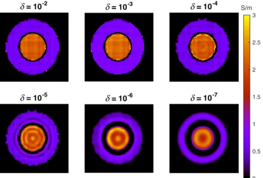
Figure 3 shows the resultant conductivity maps for varying values of d. For values of d¼ ½102;103;104
the conductivity maps are nearly identical. Some cross-hatching is visible, but we believe this is simulation arti-fact. Conductivity maps calculated with values ofd clos-er to zclos-ero result in more ringing and a loss of the sharp transition between compartments. For all experiments, we used d¼103 to minimize the bias due to the DC
offset.
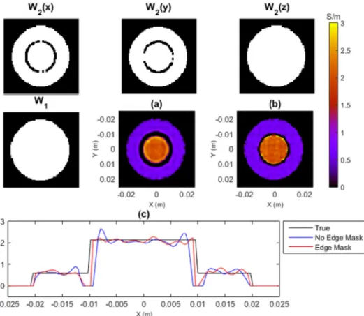
The effects of the masks used in the IL approach are shown in Figure 4. The method does not yield accurate conductivity maps when no region of support is speci-fied. This is primarily due to the lack of data in the back-ground region. Without the support mask,W1, the model
attempts to fit the sharp edge in the phase at the object border resulting in spurious conductivity values. The edge mask,W2, helps to retain information close to
mate-rial boundaries where large jumps in conductivity occur. It is clear from Figure 4 that the edge artifact at the boundary between the two materials is reduced in width by using the edge mask. Excluding the edge pixels from regularization also allows for more accurate conductivity calculations adjacent to these pixels because the transi-tion between compartments is not regularized and there-fore not encouraged to be smooth.
We assess the accuracy of each reconstruction method based on the root-mean-square error of the conductivity maps. Figure 5a shows the effect of noise in theBþ1 data on the standard deviation of the reconstructed
Table 1
Nominal and Measured Conductivity Values for Simulation and Phantom Experiments
Simulationa Phantom
Compartment Inner (S/m) Outer (S/m) Inner (S/m) Outer (S/m)
Nominal value 2.14 0.59 0.00 1.38
No erosion Filter 1.6860.88 0.4760.50 0.3460.78 1.2060.83
IL 1.9360.83 0.6560.36 0.0860.27 1.2160.84
With mask erosion Filter 2.0360.56 0.6260.49 0.1060.25 1.6560.21
IL 2.2260.33 0.7460.29 0.0160.07 1.3160.30
aReconstructed with added noise standard deviation
¼5104.
FIG. 3. Conductivity maps recon-structed with the Inverse Laplacian method for the simulation data with varying values for the offset added to the DC coefficient. No noise was added to the simulation data. The DC offset was varied between 102 and 107.
FIG. 2. Conductivity maps for the simulation experiments. AWGN was added to the complex data with standard deviation¼5104. a: True conductivity. b: Restricted Gaussian filter reconstruction. c: Inverse Laplacian reconstruction. d: Profiles throughy¼0.
conductivity map. These standard deviation values were calculated after subtracting out the mean error for the given noise level, so they provide a more accurate description of the effective conductivity map noise, removing bias due to spatially varying conductivity. The IL method produces lower conductivity standard devia-tions than the restricted Gaussian filter across all input noise levels. Figure 5b–e allow visualization of the bias associated with each reconstruction method at the lowest and highest noise levels. These are the mean error values for their respective input noise levels. The restricted
Gaussian filter yields conductivity maps with larger error near the outer edge of the object and less uniformity at higher noise levels. Figure 5d,e suggest that the IL meth-od intrmeth-oduces a slight ringing across the object. Minimal cross-hatching is visible, particularly in Figure 5b,d, due to simulation artifacts.
Phantom Data
Figure 6 shows the calculated conductivity maps for the phantom. Mean and standard deviations for each region are FIG. 4. Conductivity maps
recon-structed with the Inverse Lapla-cian method for the simulation experiments. AWGN was added to the complex data with stan-dard deviation¼104. MasksW1 and W2 are shown, where W2 provides weightings for regulari-zation in three dimensions inde-pendently.a: Only support mask,
W1, used in the reconstruction.
b: Both masks, W1 and W2, used in the reconstruction. c: Profiles throughy¼0.
FIG. 5. Measures of error due to noise and bias in both recon-struction methods. a: Standard deviation of conductivity map error as a function of the stan-dard deviation of the AWGN added to the complex simulated
Bþ
1 fields.b–e: Mean conductivity map error over all realizations for two noise standard deviation lev-els to show the bias of the Gaussian filter, (b) and (c), and Inverse Laplacian method, (d) and (e). Mean values are calcu-lated for the lowest, (b) and (d), and highest, (c) and (e), noise levels as denoted by blue dashed lines in (a).
reported in Table 1. As in the simulations, the IL method produces conductivity maps with less variation in the stant regions. Additionally, the IL method had lower con-ductivity standard deviations. For the phantom data, the inner compartment values are largely impacted by setting negative values to zero, driving the mean and standard devi-ation values closer to zero. For the outer compartment, the IL method calculated conductivity values much closer to the measured value, especially after mask erosion.
In Vivo Data
Figure 7 shows the conductivity maps for a representa-tive healthy volunteer subject. Mean and standard devia-tions for each tissue type in all four subjects, as well as across all subjects, are reported in Table 2. The ven-tricles are well-defined as is gray matter surrounding the sulci. The IL method resulted in lower values of the standard deviation within a tissue type for most subjects, particularly the white matter values. The IL method pro-duced higher standard deviations for the gray matter and CSF in two of the four subjects, which may be a result of poor definition between gray matter and CSF in the con-ductivity maps whereas the tissue segmentation is well-defined.
DISCUSSION
Conductivity mapping suffers from poor SNR because conductivity is proportional to the noise-amplifying Lap-lacian of the phase. In addition, phase-based conductivi-ty mapping generally assumes that the conductiviconductivi-ty is locally constant, an assumption that is not valid at or near tissue boundaries or in other regions of spatially varying conductivity. In a complex structure such as the brain, these boundary errors can greatly impact the accu-racy of the results. For a simple filtering method, there
exists a trade-off between SNR and edge artifacts and one must select a filter size that adequately balances the two. In our proposed Inverse Laplacian method, we have selected a regularization parameter that matches the spa-tial resolution properties of our method to those of a Gaussian filter for comparison. However, we have reduced the standard deviation of the conductivity val-ues while retaining conductivity information very close to boundaries. The use of a priori structural information plays an important role in this reconstruction method.
Our method differs from previously proposed inverse approaches in that it is a fully 3D formulation that can be solved as a single problem. The Contrast Source Inversion approach (24) has only been demonstrated in two dimensions and the inverse approach published by Borsic et al. (25) was formulated in 3D, but computation-al load required subdivision of the problem. Our ccomputation-alcula- calcula-tion of the IL filter provides a manageable problem size for the inverse approach, even for 3D volumes. An important parameter in the IL filter calculation is select-ing a small DC offset, d, so that the discrete Laplacian operator is invertible. As shown in Figure 3, we have selected a value from a wide range of possibilities that will minimize error due to this DC offset.
Based on Figure 4, the edge mask, W2, improves the
accuracy of conductivity maps near material boundaries. Without this mask, we observe a roll-off near compart-ment boundaries where the conductivity is not locally constant, yet the regularizer enforces a smooth transition. This effect is more pronounced in regions where conduc-tivity variation with space is large, such as the compart-ment boundary in the simulations or at the boundary of CSF in the brain. These regions also provide good con-trast in the MRI magnitude images, making it easy to detect the edges. Other regions of spatially varying con-ductivity may be more difficult to identify, but they FIG. 6. Conductivity maps for the experimental phantom. a: True conductivity. b: Restricted Gaussian filter reconstruction. c: Inverse Laplacian reconstruction.
cause smaller errors so it is not as important to capture those areas in the edge mask.
Boundary errors can have a large impact in comparing reconstruction methods. The conductivity values reported in Table 1 for the simulation data show that the IL method
mean values changed less with the mask erosion, support-ing the idea that the IL method can better recover conduc-tivity information near boundaries. The boundary errors in the Gaussian filter reconstruction are primarily due to applying the Laplacian operator across boundaries and are Table 2
Nominal and Measured Conductivity Values for Four Volunteer Subjects
Nominal value Measured value—Gaussian Measured value—IL
Tissue (S/m) Mean6S.D. (S/m) Mean6S.D. (S/m)
Subject 1 Gray Matter 0.59 2.4764.25 2.2962.30
White Matter 0.34 0.7860.75 0.7860.69
CSF 2.14 13.56645.76 3.0862.47
Subject 2 Gray Matter 0.59 1.4061.58 0.9661.82
White Matter 0.34 0.8160.64 0.2460.37
CSF 2.14 1.5262.61 2.2864.60
Subject 3 Gray Matter 0.59 1.4261.52 1.0961.33
White Matter 0.34 0.6460.58 0.2660.37
CSF 2.14 1.3262.10 1.1361.85
Subject 4 Gray Matter 0.59 1.2261.18 1.3161.26
White Matter 0.34 0.5860.54 0.3360.46
CSF 2.14 1.3962.40 1.6662.47
All subjects Gray Matter 0.59 1.6262.41 1.3861.70
White Matter 0.34 0.7160.66 0.4560.52
CSF 2.14 1.97610.22 1.6562.87
Nominal values from (35). FIG. 7. Spin Echo magnitude image (Row 1); tissue segmenta-tion (Row 2) showing CSF [red], white matter [yellow], and gray matter [blue]; and conductivity maps reconstructed using the restricted Gaussian filter (Row 3) and the Inverse Laplacian meth-od (Row 4) for a representative healthy volunteer subject. Each column corresponds to a differ-ent slice in the acquired volume.
propagated by filtering. One might consider excluding these regions from the Laplacian calculation, but this would still result in inaccurate conductivity values at those spatial locations.
The phantom results show that the regularization parameters translated well from simulation to phantom data, which is an encouraging result for a method that could potentially be highly dependent on parameter tun-ing. The phantom benefits from having a physical layer of separation between the two compartments, aiding in the detection of edges for maskW2. There is a
conductiv-ity spike near the compartment boundaries present in both methods, shown in Figure 6. The inner compart-ment is deionized water, so the SNR for the Bþ1 data is
lower than in the outer compartment. Coupled with the lower conductivity, this makes it more challenging to tease out the underlying curvature from the noisy data. While much of the inner compartment was set to zero in postprocessing, the IL algorithm produced fewer high conductivity values in the inner compartment.
For the human brain experiments, we present repre-sentative conductivity maps in Figure 7. The ventricles are well-defined along with many of the sulci. Similar to previous results, the Gaussian filter produced higher variation in conductivity values as compared to the IL method. A combination of filters on the phase data as well as the conductivity maps would be necessary to achieve better results, but when cascading filters one also risks loss of spatial resolution. The mean and stan-dard deviation of each tissue type for all four subjects are presented in Table 2. Mean tissue conductivity var-ied between subjects, but were generally close to reported values. Marked differences between mean tis-sue values for the Gaussian filter versus the IL method might be explained by large positive values near edges. Definition between tissue types might be improved with high resolution Bþ1 maps. Since our proposed method provides reduced noise amplification while maintaining spatial resolution properties, we can expect the IL method would be able to reconstruct accurate conductivity maps from high resolution, lower SNRBþ1 data.
CONCLUSIONS
We have developed a novel 3D regularized, model-based algorithm for phase-based conductivity mapping that uses a priori structural information to increase the accu-racy of the maps. The Inverse Laplacian method exhibits less noise amplification and better edge responses than filtering methods and has proven successful in simula-tion, phantom, and the human brain. Accurate conduc-tivity maps are essential for subject-specific conducconduc-tivity calculations to be valuable in clinical or safety applica-tions. To improve the accuracy of our method, we plan to investigate the incorporation of nonconstant electrical properties into the system model. This would be equiva-lent to deriving a system model from the Helmholtz equation as opposed to the homogeneous version. We believe this would result in more accurate values in regions with spatially varying electrical properties,
specifically at the locations we have excluded from regu-larization in the current methodology.
ACKNOWLEDGMENT
The authors would like to acknowledge academic license support for SEMCADX by SPEAG, www.speag.com. REFERENCES
1. Zhang X, Zhu S, He B. Imaging electric properties of biological tis-sues by RF field mapping in MRI. IEEE Trans Med Imaging 2010;29: 474–481.
2. Voigt T, Vaterlein O, Stehning C, Katscher U, Fiehler J. Electrical conductivity imaging of brain tumors. In Proceedings of the 19th Annual Meeting of ISMRM, Montreal, Canada, 2011. p. 127. 3. Shin J, Kim MJ, Lee J, Nam Y, Oh Kim M, Choi N, Kim S, Kim DH.
Initial study on in vivo conductivity mapping of breast cancer using MRI. J Magn Reson Imaging 2014;42:371–378.
4. van Lier ALHMW, Raaijmakers A, Voigt T, Lagendijk JJW, Luijten PR, Katscher U, van den Berg CAT. Electrical properties tomography in the human brain at 1.5, 3, and 7T: a comparison study. Magn Reson Med 2014;71:354–363.
5. Miranda PC, Hallett M, Basser PJ. The electric field induced in the brain by magnetic stimulation: a 3-D finite-element analysis of the effect of tissue heterogeneity and anisotropy. IEEE Trans Biomed Eng 2003;50:1074–1085.
6. Wagner TA, Zahn M, Grodzinsky AJ, Pascual-Leone A. Three-dimen-sional head model simulation of transcranial magnetic stimulation. IEEE Trans Biomed Eng 2004;51:1586–1598.
7. Wagner T, Fregni F, Fecteau S, Grodzinsky A, Zahn M, Pascual-Leone A. Transcranial direct current stimulation: a computer-based human model study. NeuroImage 2007;35:1113–1124.
8. Sadleir RJ, Vannorsdall TD, Schretlen DJ, Gordon B. Transcranial direct current stimulation (tDCS) in a realistic head model. Neuro-Image 2010;51:1310–1318.
9. Voigt T, Katscher U, Doessel O. Quantitative conductivity and per-mittivity imaging of the human brain using electric properties tomog-raphy. Magn Reson Med 2011;66:456–466.
10. van Lier AL, Hoogduin JM, Polders DL, Boer VO, Hendrikse J, Robe PA, Woerdeman PA, Lagendijk JJ, Luijten PR, van den Berg CA. Elec-trical conductivity imaging of brain tumors. In Proceedings of the 19th Annual Meeting of ISMRM, Montreal, Canada, 2011. p. 4464. 11. Bulumulla S, Hancu I. Breast permittivity imaging. In Proceedings of
the 20th Annual Meeting of ISMRM, Melbourne, Australia, 2012. p. 4175.
12. Katscher U, Djamshidi K, Voigt T, Ivancevic M, Abe H, Newstead G, Keupp J. Estimation of breast tumor conductivity using parabolic phase fitting. In Proceedings of the 20th Annual Meeting of ISMRM, Melbourne, Australia, 2012. p. 2335.
13. Katscher U, Abe H, Ivancevic MK, Keupp J. Investigating breast tumor malignancy with electric conductivity measurement. In Pro-ceedings of the 23rd Annual Meeting of ISMRM, Toronto, Canada, 2015. p. 3306.
14. Haacke EM, Petropoulos LS, Nilges EW, Wu DH. Extraction of con-ductivity and permittivity using magnetic resonance imaging. Phys Med Biol 1991;36:723–734.
15. Katscher U, Voigt T, Findeklee C, Vernickel P, Nehrke K, Dossel O. Determination of electric conductivity and local SAR via B1 map-ping. IEEE Trans Med Imag 2009;28:1365–1374.
16. Wen H. Non-invasive quantitative mapping of conductivity and dielectric distributions using the RF wave propagation effects in high field MRI. In Proceedings of SPIE 5030, Medical Imaging 2003: Phys-ics of Medical Imaging, San Diego, California, USA, 2003. pp. 471– 477.
17. Seo JK, Kim MO, Lee J, Choi N, Woo EJ, Kim HJ, Kwon OI, Kim DH. Error analysis of nonconstant admittivity for MR-based electric prop-erty imaging. IEEE Trans Med Imaging 2012;31:430–437.
18. Duan S, Xu C, Deng G, Wang J, Liu F, Xin SX. Quantitative analysis of the reconstruction errors of the currently popular algorithm of magnetic resonance electrical property tomography at the interfaces of adjacent tissues. NMR Biomed 2016;29:744–750.
19. Gurler N, Ider YZ. Gradient-based electrical conductivity imaging using MR phase. Magn Reson Med 2017;77:137–150.
20. Hafalir FS, Oran OF, Gurler N, Ider YZ. Convection-reaction equation based magnetic resonance electrical properties tomography(cr-MREPT). IEEE Trans Med Imaging 2014;33:777–793.
21. Liu L, Zhang X, Schmitter S, de Moortele PFV, He B. Gradient-based electrical properties tomography (gEPT): a robust method for map-ping electrical properties of biological tissues in vivo using magnetic resonance imaging. Magn Reson Med 2015;74:634–646.
22. Liu J, Zhang X, Wang Y, de Moortele PFV, He B. Local electrical properties tomography with global regularization by gradient. In Pro-ceedings of the 23rd Annual Meeting of ISMRM, Toronto, Canada, 2015. p. 3297.
23. Huang L, Schweser F, Herrmann KH, Kramer M, Deistung A, Reichenbach JR. A Monte Carlo method for overcoming the edge arti-facts in MRI-based electrical conductivity mapping. In Proceedings of the 22nd Annual Meeting of ISMRM, Milan, Italy, 2014. p. 3190. 24. Balidemaj E, van den Berg CA, Trinks J, van Lier AL, Nederveen AJ,
Stalpers LJA, Crezee H, Remis RF. CSI-EPT: A contrast source inver-sion approach for improved MRI-based electric properties tomogra-phy. IEEE Trans Med Imaging 2015;34:1788–1796.
25. Borsic A, Perreard I, Mahara A, Halter RJ. An inverse problems approach to MR-EPT image reconstruction. IEEE Trans Med Imaging 2016;35:244–256.
26. Sodickson DK, Alon L, Deniz CM, et al. Local maxwell tomography using transmit-receive coil arrays for contact-free mapping of tissue electrical properties and determination of absolute RF phase. In Pro-ceedings of the 20th Annual Meeting of ISMRM, Melbourne, Austra-lia, 2012. p. 387.
27. Sodickson DK, Alon L, Deniz CM, Ben-Eliezer N, Cloos M, Sodickson LA, Collins CM, Wiggins GC, Novikov DS. Generalized local maxwell tomography for mapping of electrical property gradients and tensors. In Proceedings of the 20th Annual Meeting of ISMRM, Melbourne, Australia, 2012. p. 2532.
28. Serralles JE, Polimeridis A, Vaidya MV, Haemer G, White JK, Sodickson DK, Daniel L, Lattanzi R. Global maxwell tomography: a novel technique for electrical properties mapping without symmetry
assumptions or edge artifacts. In Proceedings of the 24th Annual Meeting of ISMRM, Singapore, 2016. p. 2993.
29. Charbonnier P, Blanc-Feraud L, Aubert G, Barlaud M. Two determin-istic half-quadratic regularization algorithms for computed imaging. In Proceedings of IEEE International Conference on Image Processing, 1994, volume 2. pp. 168–171.
30. Panin VY, Zeng GL, Gullberg GT. Total variation regulated EM algo-rithm. IEEE Trans Nucl Sci 1999;46:2202–2210.
31. Fessler JA. Image reconstruction toolbox. Available at: http://web. eecs.umich.edu/fessler/code/index.html. Accessed February 1, 2013.
32. Kim DH, Choi N, Gho SM, Shin J, Liu C. Simultaneous imaging of in-vivo conductivity and susceptibility. Magn Reson Med 2014;71:1144–1150. 33. Xu W, Cumming I. A region-growing algorithm for InSAR phase
unwrapping. IEEE Trans Geosci Remote Sens 1999;37:124–134. 34. Wellcome Trust Centre for Neuroimaging. Statistical parametric
map-ping. Available at: http://www.fil.ion.ucl.ac.uk/spm/. Accessed April 1, 2016.
35. Hasgall PA, Di Gennaro F, Baumgartner C, Neufeld E, Gosselin MC, Payne D, Klingenb€ock A, Kuster N. IT’IS database for thermal and electromagnetic parameters of biological tissues. Version 2.4 2013. doi: 10.13099/VIP21000-03-0.
SUPPORTING INFORMATION
Additional Supporting Information may be found in the online version of this article.
Fig. S1.Comparison of spatial resolution for each reconstruction method. For a given PSF width we are able to select corresponding regularization parameter and filter standard deviation. Selected parameters are denoted by the dotted line.
Fig. S2.Fraction of conductivity images used to calculate mean values after eroding the compartment masks with a 939 pixel square. Simulation reconstructed with (a) restricted Gaussian filter and (b) Inverse Laplacian method. Phantom reconstructed with (c) restricted Gaussian filter and (d) Inverse Laplacian method.

![FIG. 7. Spin Echo magnitude image (Row 1); tissue segmenta-tion (Row 2) showing CSF [red], white matter [yellow], and gray matter [blue]; and conductivity maps reconstructed using the restricted Gaussian filter (Row 3) and the Inverse Laplacian meth-od (](https://thumb-us.123doks.com/thumbv2/123dok_us/443327.2551297/9.918.93.836.850.1114/magnitude-segmenta-conductivity-reconstructed-restricted-gaussian-inverse-laplacian.webp)