Market Price Analysis
and Risk Management
for Convertible Bonds
Fuminobu Ohtake, Nobuyuki Oda
and Toshinao Yoshiba
Fuminobu Ohtake: Market Risk Management Division, Bank of Tokyo–Mitsubishi (E-mail: fuminobu_otake@btm.co.jp)
Nobuyuki Oda and Toshinao Yoshiba: Research Division 1, Institute for Monetary and Economic Studies, Bank of Japan (E-mail: nobuyuki.oda@boj.or.jp, toshinao.yoshiba@ boj.or.jp)
This paper is an expansion and revision of a paper originally submitted to a research workshop on “Analyses of Stock Market Using Financial Engineering Techniques” held by the Bank of Japan in July 1998. The authors wish to emphasize that the content and opinions in this paper are entirely their own and do not represent the official positions of either the Bank of Tokyo–Mitsubishi or the Bank of Japan.
This paper discusses pricing methods, comments on matters of concern in market risk management, and analyzes market characteristics of convertible bonds.
Valuation of the conversion option is essential in analyzing the market price of a convertible bond. In this paper, we use a binomial tree pricing model to derive the implied volatility of the conversion option from the past price information (time-series data for individ-ual issues) in the Japanese market. We then use this implied volatility data: (1) to employ a Monte Carlo simulation to measure market risk for a test portfolio of convertible bonds and analyze the factors in price fluctuation; and (2) to perform regression analyses that empirically verify the characteristics of the convertible bond market in Japan.
The implication for market risk management is to underscore the need to be aware of market price fluctuation caused by implied volatility fluctuation. We found that in markets such as Japan is experiencing at the present time, in which most issues have little linkage to share price movements, there is a particular need to be aware of implied volatility in risk management. Moreover, our analysis of market characteristics found that (1) there is a significant negative correlation between implied volatility and underlying equity price fluctuation; (2) implied volatility tends to move in such a way as to reduce divergence from the historical volatility of the underlying equity price; and (3) the use of convertible bonds to raise funds during the “bubble” period in Japan was not necessarily an advantageous form of financing for the issuers.
Key words: Convertible bond; Implied volatility; Historical volatility; Market risk; Arbitrage; Issuing conditions
I. Introduction
It should be axiomatic that anyone trading financial instruments, whether dealers (market makers) or investors (end users) should be concerned with obtaining “fair value” for the trade. Estimates of fair value generally involve the use of some sort of pricing model, and the prices that these models come up with are used by the front office to search for mispricing in the markets, with appropriate hedges for risk. The middle office will also use these prices in risk control and capital allocation. This applies to convertible bonds, the subject of this analysis.
Convertible bonds1 are hybrid instruments that are part bond and part equity
(stock option). The key to pricing them is to apply option price theory (to the equity portion) and credit risk evaluation (to the bond portion). Recent years have seen an increase in the number of complex convertible bond instruments on the market, generally with clauses that provide for revisions in the conversion price. The handling of these instruments requires fairly advanced technology, particularly for the pricing of the option portion. Unfortunately, few papers have attempted to create a systematic methodology for pricing convertible bonds. This paper therefore has three goals: (1) to provide a theoretical explanation of convertible bond pricing and an empirical analysis of that theory; (2) to note points of concern in market risk management; and (3) to consider the implications regarding market characteristics.
The structure of this paper is as follows. Chapter II begins with a discussion of convertible bond pricing theory, followed by examples of pricing models that can be used in practical situations. We use these models for some convertible bonds to analyze market risks and price fluctuation factors, demonstrating that the conversion option in convertible bonds contains elements that cannot be ignored when manag-ing market risks. Chapter III uses implied volatility to perform an empirical analysis of the conversion option in convertible bonds. To this, we add some observations on the characteristics of the Japanese convertible bond market. Finally, Chapter IV provides some brief conclusions.
II. Convertible Bond Pricing Theory and Market Risk
Measurements
This chapter contains a theoretical discussion of convertible bond pricing methods, followed by a practical analysis of market risk measurements. We begin with a brief review of the salient characteristics of convertible bonds as financial instruments, and move from there to pricing models that could be used. We then go on to create a test
1. Bonds with warrants are another financial instrument that is often discussed in conjunction with convertible bonds, but we do not deal with them in this paper. Bonds with warrants are generally split into warrants and straight bonds (ex-warrant bonds) when traded, and because the two portions can be priced separately they are much easier to deal with than convertible bonds. Similarly, convertible bonds seem to lend themselves more to exotic instruments with complex features than do bonds with warrants. In light of these considerations, we will concentrate only on convertible bonds in this paper. For a basic discussion of pricing methods for bonds with warrants, the reader is referred to Hull (1997) and Takahashi (1996).
convertible bond portfolio, measuring the market risks in terms of “value at risk,” and elucidating from this some points of concern in risk management.
A. Basic Characteristics of Convertible Bonds
This section provides a brief overview of the basic schemes and product character-istics of convertible bonds.
Convertible bonds are a form of bond issued by companies that comes with the right to convert the bond into ordinary shares in the issuer2 according to preset
conditions (conversion provision). The most common form of conversion provision is to establish a specific conversion period prior to the maturity of the bond (this conversion period corresponds to the exercise period for American options). As long as it is within the designated period, the investor may demand that his bonds be exchanged for ordinary shares at a preset ratio. This ratio is called the “conversion ratio.” The value obtained were the bonds to be exchanged for shares at the present time according to the preset conversion ratio is called “parity.” The price paid per share in terms of the par amount of the convertible bond to buy the common stock is referred to as the “conversion price.” For example, if the convertible bond has a par value of ¥1,000, the current share price is ¥400, and the conversion ratio is two, then parity is ¥800 and the conversion price is ¥500. In other words,
Parity = underlying asset price ×conversion ratio. Conversion price = par value/conversion ratio.
The difference between the price of the convertible bond and parity is the “conversion premium”:
Conversion premium = (convertible bond price – parity)/parity ×100.
When the market price of a convertible bond is below parity, it is trading at a “conversion discount.”
This is the most basic scheme for this instrument. In recent years, a growing number of convertible bonds have been issued with additional conversion provisions. Below is a discussion of some of the most common of these provisions.
1. Call provision
This provision enables prior redemption of the bond at a set price after the time remaining to maturity falls below a preset threshold (generally about three or four years). This provision has often been added to Japanese convertible bonds, but practice in the market has been to assume that the provision would not in fact be exercised under ordinary circumstances, and there are indeed only a few examples of the provision being used to accelerate redemption (the bonds being “called”).
2. As exceptions to this rule, some schemes allow conversion to equity from a different company than the issuer. These are called exchangeable bonds. In such schemes, there are no new shares issued as there would be with an ordinary convertible bond; rather, the issuer of the convertible bond delivers shares in another company that it already holds. One example of how an exchangeable bond could be used would be an issuer that wants to liquidate its holdings in an affiliate but does not want to sell the shares directly to the market.
Investors have therefore considered the call provision to have no real economic significance and have not incorporated its effects in pricing.
However, since 1996 there have been several bonds issued with new call provi-sions (for example, the “130 percent call option”3). This provision is set under the
assumption that it might actually be exercised, and so this conversion provision should be reflected in the valuation of the option.
2. Provision allowing downward revisions in the conversion price
This provision makes it possible to revise the conversion price downward after a set period of time has elapsed since issue. It therefore has the effect of increasing the conversion potential. For investors, it has the benefit of resuscitating convertible bond prices that have fallen because sliding share prices have reduced the value of the option, while for the issuer it has the benefit of encouraging conversion to take place (assuming that is what the issuer wants). However, it also exposes shareholders to the risk that there will be a dilution in the value of their shares since a revision in the conversion price will change the number of latent shares in the company. Analyses that seek precision must therefore take this dilution effect into account (see Footnote 13).4
Convertible bonds with these provisions first emerged in the Japanese market after the 1996 deregulation, and indeed, just under 30 percent of the convertible bonds issued that year had some form of additional feature.5
3. Provision providing for forced conversion at maturity
This provision provides for forced conversion to equity at a preset conversion ratio (in some schemes, this ratio may be revised prior to maturity) of all convertible bonds that remain unconverted when the bond matures. The forced conversion provision is exercised regardless of the wishes of convertible bondholders and issuers. It is found on almost all of the convertible bonds, subordinated debt, and preferred shares issued by Japanese banks over the last two or three years.
However, one of the problems with this provision is that if the latent shares are converted all at once, there is a very real potential to harm the supply and demand balance for the stock and spark a crash in its price. To avoid this, some issues have used forced conversion provisions that spread conversion throughout the life of the bond rather than leaving it all for maturity.
B. Pricing Theory
Professionals generally use two kinds of convertible bond pricing model. The first calculates a theoretical fair value at the time of valuation assuming no arbitrage. This corresponds to the Black-Scholes model in stock options. The second model attempts to identify all factors that have an influence on pricing and model their impact. It is
3. This provision only allows the call option to be exercised if parity is at 130 or higher. For example, if Nissho Iwai No. 1 is at a parity of 130 or higher for 20 days running, then the issuer will be able to accelerate redemption at an exercise price of ¥100.
4. For an analysis of the effect on share prices from convertible bonds issued by banks with additional features (the ability to revise the conversion price downward, etc.), see Kamata and Yarita (1997).
therefore called a “multifactor model.”6 Multifactor models are generally used to
estimate future price trends. This paper will therefore concentrate on the first type of pricing model.
The equation below provides a more intuitive grasp of the basic framework for pricing:7
Convertible bond price (CB) = bond value (B) + equity option value (OP). The discussion below explains the pricing model that is used to value the right side of this equation. There are many variations to the model, however, and the choice of which to use will involve a trade-off between accuracy of valuation and complexity of calculation. Our discussion will begin with the simplest and most approximate model (the “simple model”), explaining in the course of the discussion which points it approximates on. We will then discuss a revised model that eliminates the approximated elements, though here again we must emphasize that there is no one best way to revise the simple model. To give the reader some idea of the breadth available, we will consider three types of model found in the professional literature.
1. The simple model
The easiest way to price convertible bonds is to value the bond and equity option components separately. The value of the bond component (B) is the total present value of all future cash flow from a discounted interest rate found by adding the spread8 at the time of valuation on the riskless rate. The value of the equity option
component (OP) is handled as the theoretical price (under the Black-Scholes formula) of a call option that uses parity at the time of valuation for the underlying asset price and the par value of the convertible bond as the exercise price. In mathematical form, therefore, the price of the convertible bond (CB) would be
CB= B+OP. T CFt B=
∑
———————— . t=1 [1 + RF(t) + SP(t)]t OP= x.N(d) –k.e–RF(T)T.N(d – σ√T).6. Below is the basic form that a multifactor model would take for the rate of return on a security (traditionally, an equity): M R~j= RF+ ∑xj,kF ~ k+ e~j. k=1
In this equation, R~jstands for the rate of return on security j, F
~
kfor the value of factor k(the factor return), xj,k
for the sensitivity of security jto factor k(the factor exposure), RFfor the riskless interest rate, and e~jfor the error.
The actual types of factors and exposures that will appear on the right-hand side of the equation depend on the empirical analysis on which the model is based. One common example is the Barra model of the rate of share price returns. The Nikko-Barra CB Risk Model is an example of an attempt to apply this framework to estimates of the rate of return on convertible bonds. For further discussion, see Miyai and Suzuki (1991).
7. In point of fact, convertible bonds never strip the equity option component off the bond component and trade the two separately (in this, they differ from bonds with warrants). The two will affect each other in pricing, so it is not, strictly speaking, appropriate to value them separately. We must therefore emphasize that this discussion (and the many similar discussions found in the literature) is employed merely as a matter of convenience.
8. Appropriate spreads are determined at the time of valuation with reference to the market prices of other bonds of similar credit risk and liquidity risk.
x 1 ln— + [RF(T) + —σ2]T
k 2
d ≡—————————— .
σ√T
In this equation, CFtstands for the cash flow for termt, RF(t) for the riskless rate for
termt, SP(t) for the spread corresponding to termt, x for parity,k for the par value of the convertible bond, σfor share price volatility, T for the final day in the conver-sion period, and N(•) for the cumulative probability density function for a standard
normal distribution.
Should the share price be far above the conversion price (parity far higher than the par value of the convertible bond),then x/k >> 1, which will make the relationship
N(d) ≈1, N(d – σ√T) ≈1 true. From this, we can conclude
CB ≈x+ (B– k.e–RF(T)T).
When the effect of the coupon and spread for the bond component is sufficiently smaller than the equity option component, it is possible to abstract the second clause in the equation above to give the relationship CB ≈ x. What this expresses is that when the equity option component is “deep in the money,” then the convertible bond price will be roughly at parity (Figure 1). On the other hand, if the share price is far below the conversion price (if parity is far below the par value of the convertible bond), then the option price will be close to zero so the relationship CB ≈B will hold. What this expresses is that when the equity option component is “far out of the money,” then the convertible bond price will more or less match the price of the bond component. This behavior is indeed observed in the markets and holds true apart from the limits to the simple model described below.
Next we would explain the limits to the simple model. We would underscore the fact that it uses approximation on two basic points.9
120 Price
Convertible bond price (CB )
Parity (x ) Parity Bond value (B ) 70 80 90 100 110 115 110 105 100 95 90 85 80 Equity option value (OP ) Figure 1 Convertible Bond Price Curve
9. In point of fact, there are reports that a method of convenience like the simple model provides unsatisfactory results when it is necessary to calculate extremely accurate prices (for example, Shoda [1996]).
(1) It fixes the exercise price when valuing the equity option
In convertible bonds, the exercise of the option enables one to receive a value equivalent to parity (in the form of shares), in exchange for which one pays a value equivalent to the bond (in the form of the bonds themselves). The value of the bond will depend on interest rates (term structure) and spreads at the time of exercise and cannot be forecasted with any certainty ahead of time. In spite of this, the simple model assumes that bonds are at par value at the time of exercise (that the bond price is equal to the par value).
To remedy this approximation, it is necessary to use a model that allows both the exercise price (bond price) and the underlying asset price (share price) to fluctuate over the stochastic process. Generally speaking, modeling the stochastic process of future bond prices requires the use of some form of yield curve model.10Note that when a relatively simple model is used in which
bond prices themselves follow the lognormal process, it is possible to apply exchange option pricing theory.11
The credit risk premium is one factor in determining the price of the bond at the time of exercise, but this will also be related to trends for the underlying shares (or parity).12 For example, if the underlying shares have dropped in
price after the convertible bond was issued, then the credit risk spread will be larger than it originally was (assuming there has been no change in the riskless rate), so the bond price that serves as the exercise price will also be falling. This linkage is abstracted in the simple model.
(2) It assumes European options for the equity options
Convertible bonds generally allow options to be exercised within a set conver-sion period, which makes them suited to valuation as American-style options. However, for analytical convenience, the simple model treats them as if they were European-style options.
Accurate valuation of American options generally requires the use of lattice methods (binomial trees or finite difference methods).
The model below attempts to remedy these approximated elements.13
10. For a discussion of yield curve models, see Hull (1997).
11. An exchange option is defined as an option that exchanges two different assets (for our purposes, stocks and bonds). If it is assumed that both asset prices will follow a lognormal process, then it is known that there is an analytic solution, particularly for European options (Margrabe [1978]). However, attempting to use a lognormal process for bond prices, as we do in this example, involves making some rather strong assumptions, for instance, it leaves one unable to take account of the mean reversion of interest rates. It may therefore produce unrealistic results, especially if it is used for analyses with long time horizons.
12. For an analysis of the relationship between bond ratings and share prices, see Suzuki (1998).
13. Actually, there are other approximations in the simple model besides the two discussed. For example, it does not take account of dilution effects. We will not delve too deeply into this issue here, but to provide a brief explana-tion, there are three basic patterns by which the issue of new shares can affect the share price (for our purposes here, we will not consider the signaling effect of new share issues): (1) issues above market will raise the share price; (2) issues at market will have no impact on the share price; and (3) issues below market will lower the share price. Convertible bond options are only exercised (bonds are only converted into shares) when parity (or the share price) is below the par value of the convertible bond (or the conversion price), so this is basically an issue of (3) above. Because of this, a higher expectation of conversion will produce downward pressure on the share price. This is known as the “dilution effect.” The size of the dilution effect will depend on the spread between the share price and the conversion price at the time of conversion and on the number of new shares converted.
2. Calculations using binomial trees
Binomial trees can be used to overcome part of the first problem and all of the second. The framework for this method involves valuing the price of a convertible bond by rolling back through a comparison of the value when the conversion option is exercised (parity) and the value when the convertible bond is held for each node (an expression designating a time-state pair) along a tree. This technique makes it possi-ble to value convertipossi-ble bonds with issuer call provisions. Below is an explanation of the process in more detail.
Step 1: Create a parity tree
For a convertible bond with no conversion price revision features, there will be no change in the conversion ratio, which makes it easy to create a parity tree just by creating a share price tree and performing a few simple calculations. First, one creates a share price tree under risk-neutral probability (Figure 2).
This allows us to calculate u, d, and pusing the following equations:
u= exp(σ√∆t).
d= exp(–σ√∆t). exp[(r–q)∆t] –d
p= ———————.
u–d
That is enough to build the share price tree. From there, it is just a matter of multiplying the share price by the conversion ratio to create a parity tree (see Section II.A).
Step 2: Calculate the convertible bond price for each node (a) Calculate price at maturity
Comparisons of bond prices and parities at the time the convertible bond matures will give the value for each node at the time of maturity. The following equation is used to do this in order to take into account the impact of call and put provisions.
S : present share price u : share price upward rate d : share price downward rate p : transition probability q : dividend rate
r : riskless rate
σ: share price volatility
∆t : length of one term Su2 Su Sd 1– p 1– p 1– p 1–p 1–p 1– p Sud = S S
Figure 2 Binomial Tree of Share Prices
FVCB(T, i) = max[Z(T, i), P(T), min(C(T), B(T, i))].14
Note that the suffix tdesignates time (t = 0, 1, . . . T, T= maturity) and the suffix
i indicates state (i = 1, . . . , t + 1), so that the convertible bond price, parity, put price, and call price at each node (t, i) are expressed as FVCB(t, i), Z(t, i), P(t), and
C(t), respectively, and the bond price at maturity is expressed as B(T, i).
(b) Roll back through the node calculations
Use the maturity values (at each state i) found in sub-step (a) to calculate the expected present value for the node one time period prior. If the maturity state is “bond,” then calculate present value (PVi
t) using a discount rate that takes account of
credit risk by adjusting the riskless rate for a credit spread; if it is equity conversion, then use a simple riskless rate for the discount rate. Following this, use transition probability (p) to calculate the expected price as a bond (X(t, i)). Then calculate the conversion price for each node using the same methods as for sub-step (a):
X(t, i) = pPVi
t(FVCB(t+ 1, i)) + (1 –p)PVti+1(FVCB(t+ 1, i + 1)). FVCB(t, i) = max[Z(t, i), P(t), min(C(t), X(t, i))].
A backward induction that repeats these steps until the present time (t= 0) is arrived at will yield the present price.
The binomial tree method is better, but not without its problems since it still does not account for the possibility of changes in the future riskless rate, and it treats the credit risk spread as if it were certain.15
3. Pricing models that consider firm values
Another model that remedies part of the first problem and all of the second problem in the simple model described above is the OVCV convertible bond model developed and provided by Bloomberg.16 This pricing model focuses on firm values, and its
approach is to consider the convertible bond to be an option underlaid by the firm values.17What sets this model apart is that it explicitly values the extent of net debt in
the event of default, and in doing so makes the credit risk on the bond component of the convertible bond endogenous to the model. Still, this model has problems too, since it assumes Brownian motion for corporate values and reverts to the simple model in order to simplify calculations to the point of practical utility.18
14. This assumes that if the issuer, as a rational course of action, exercises its right to accelerate redemption under the call provision, the investor who recognized this would exercise the conversion option (or exercise the put provision) prior to actual redemption.
15. Another pricing model that uses a binomial tree is found in Cheung and Nelken (1994), which draws on exchange option concepts. This is a two-factor model that treats both share prices and interest rates as random variables. In its use of trees for American options, it is similar to the model described in Section II.B.2, but because it uses two random variables, the image is one of creating two differing binomial trees.
However, it also assumes that interest rates and share prices are independent of each other, and it applies the measured credit risk spread at the present time as a fixed value in the future.
16. See Oi (1997), Gupta (1997), and Berger and Klein (1997a, b) for outlines of the OVCV. 17. See Brennan and Schwartz (1977) and Ingersoll (1977) for further discussion.
4. Methods of valuing exotic convertible bonds
In Section II.A, we noted that a growing number of convertible bonds in Japan were issued with additional features attached. It appears that many nonfinancial issuers attach conversion price revision features, while bank issuers attach not only conversion price revision features but forced conversion at maturity provisions as well. Bank convertible bonds, in particular, are issued primarily as a means of raising capital that can be counted toward Bank for International Settlements (BIS) capital-adequacy standards, and this provides much of the motivation for the forced conversion provision.19
Pricing theory finds it ineffective to use recombination lattice methods for path-dependent instruments (derivatives that follow non-Markov processes). General practice is to use Monte Carlo simulation instead. On the other hand, Monte Carlo simulation (which assumes forward induction) is unsuited to American-style options (which require backward induction), so standard practice for American-style options is to use lattice methods. Unfortunately, the instruments we are dealing with in this subsection are path-dependent American-style options, so further extensions will be required. Among the possible approaches to dealing with this would be to follow Hull (1997) in creating an approach that takes account of path-dependence while also attempting to reduce calculation burdens within the grid framework. Another would be to create a grid model that does not recombine and, if dealing with a clause permitting only downward revisions to the conversion price, use a Monte Carlo simulation that does not assume that investors will exercise prior to term.
However, we should point out that there are a wide variety of methods used to determine conversion prices (particularly with convertible bonds issued by Japanese banks), so models will have to be customized to individual issues if precision is desired in pricing.
C. Calculating Value at Risk (VaR) for Market Risks
In this section, we analyze the market risk associated with convertible bonds. More specifically, we utilize value at risk (VaR) concepts, which are the normal method employed in quantitative models of market risk, to perform calculations on a test portfolio. We then go on to note several concerns to be aware of when valuing the market risk of convertible bonds.
1. Basic points in calculating the market risk of convertible bonds
Convertible bonds are a hybrid of bonds and equities, so measurements of their market risk will need to take account of share prices, interest rates, and implied volatility as risk-generative factors. In addition, the convertible bond price is non-linear with respect to share price movements,20 so among the various methods
available to calculate VaR, Monte Carlo simulation stands out as the best in terms of accuracy, since it uses the convertible bond pricing model to calculate risk values for
19. Nor is it just convertible bonds (bonds with conversion options) that banks are issuing. They are also issuing preferred shares and subordinated debt with conversion options. For the sake of convenience, we shall refer to all of these instruments as “convertible bonds” in this paper.
changes in risk factors (differential calculations). However, Monte Carlo simulation has the drawback of unacceptably heavy calculation burdens, so there may be cases in which some simpler method is the better choice. An example of an alternative, simpler method would be to deem the convertible bond to be a delta-equivalent share price, and only calculate share price movement risk (with no attempt to value the convertible bond itself ). In this paper, we use this “simple method” alongside Monte Carlo simulation and compare the results obtained from both.
Driven by the bull market for stocks, the convertible bond market saw its number of listed issues and market capitalization grow consistently in the late 1980s, but the market began to weaken at roughly the same time that share prices peaked out; and more issues went from being driven by share prices to being driven by interest rates. This history was behind our decision to calculate VaR for post-“bubble” issues at two points in time (1994 and 1998) and use these calculations to observe the market risk inherent in convertible bonds.
2. Portfolio analysis
Below are outlines of the Monte Carlo simulation and simple method used to calculate VaR in this analysis.
Monte Carlo simulation
(1) Risk categories and risk factors
We posit three risk categories: share prices, interest rates, and implied volatility. As risk factors for share prices and implied volatility, we use data on individual issues; for interest rates, we use the yield on Japanese government bonds (0.5, 1, 2, . . . , 10 year).
(2) Generation of random numbers
We generate multivariate normalized random numbers for each risk factor and use Monte Carlo simulation techniques to measure VaR. The multivariate normalized random numbers were generated by multiplying normalized random numbers created using the Box-Muller method by a series obtained from a Cholesky decomposition21 of a correlation matrix calculated from weekly rate
of return data for a one-year observation period for each risk factor. Linear
21. The calculation of multivariate ordinary random numbers requires breaking down a positive definite and symmetric correlation matrix C(ρi j) using a matrix A(ai j) that meets the condition
C= AAT
.
For each A that satisfies this, a vector ymultiplied by an ordinary random number vector xwill produce a correlation series Cwith the same correlation structure. One simple method for seeking series Ais Cholesky decomposition, in which the components of series Aare calculated as follows:
a11= √ρ11= 1, ai1= ρi1 i= 2, 3, . . . , n j–1 aj j= ρjj– ∑a 2 jk j= 2, 3, . . . , n √ k=1 1 j–1 ai j= — (ρi j– ∑aikajk) j< i, j= 2, 3, . . . , n– 1 aj j k=1 ai j= 0, 1 ≤i<j≤n.
interpolation was used to seek interest rates when the time to maturity for the convertible bond contained fractions of years (5.5 years, etc.).
(3) Number of simulations 10,000.
(4) VaR calculation method
We input to the pricing model the multivariate normalized random number vector generated in step 2 and calculated the difference from the market value on the base date.
Expressing the risk factors (share prices, implied volatility, interest rates) for issue i as Si, IVi, and Ri, respectively, the portfolio value as P, the value of
individual convertible bonds as Vi(Si, IVi, Ri), and the multivariate normalized
random number vector for k items generated in step 2 as Xk, then Xk= (S1,k, S2,k, . . . , Si,k, IV1,k, IV2,k, . . . , IVi,k, R1,k, R2,k, . . . , Ri,k). ∆Pk=
∑
∆Vi,k=∑
[Vi(Si,k, IVi,k, Ri,k) – Vi(Si,0, IVi,0, Ri,0)].i i
k = 1, 2, . . . , 10,000.
Vi(Si,0, IVi,0, Ri,0) is the convertible bond price on the base date.
For the pricing model, we use a binomial tree. (5) VaR calculation criteria
VaR assumes a holding period of two weeks, and a bottom 99th percentile price fluctuation rate against the base date price (∆Pk/total market value on the base date).
(6) VaR calculation base dates22
July 1, 1994 and March 31, 1998.
The simple method
(1) Risk categories and risk factors
The only risk category is share prices, and the only risk factor is individual share prices.
22. To briefly summarize the convertible bond market trends for 1994 that served as the basis for our selection of these base dates:
(1) After the collapse of the “bubble,” there were large drops in equity financing (capital increases, convertible bonds, bonds with warrants), but in 1994 the stock market turned upward and this set the stage for renewed financing through convertible bonds.
(2) Institutional investors and personal investors began to buy convertible bonds in the expectation that share prices would rise, so the convertible bond market was solid until about July.
(3) Companies actively issued new equity-linked bonds to provide themselves with the resources to redeem old equity-linked bonds and to raise funds for new capital investments.
(4) In August, the convertible bond market turned downward as the increase in issues began to undermine supply and demand and the fall in coupons made convertible bonds less attractive as investments. Many issues saw their initial listing at below-par prices. The convertible bond market was slack for the rest of the year.
This environment led us to build a portfolio on the assumption that we had purchased convertible bonds at a mix reflective of the market and at a stage immediately prior to a softening of the market (stage 2).
The other base date (March 31, 1998) was selected as the most recent date for which analytical data were available.
(2) Generation of random numbers
Multivariate ordinary random numbers for each share price were generated using the same method as in Monte Carlo simulation.
(3) Number of simulations
10,000 (same as Monte Carlo simulation). (4) VaR calculation method23
We calculated the amount of change in share prices from a multivariate normal-ized random number vector of share prices and then found the multiplication of the vector of sensitivities to share prices for individual convertible bond prices. In mathematical form, this is expressed as
∂Vi,0 ∆Pk=
∑
∆Vi,k=∑
[Si,k– Si,0]——.i i ∂Si,0
Unlike Monte Carlo simulation, the simple method does not require that con-vertible bonds be revalued because risk is valued in terms of share prices. Sensitivity is calculated analytically from the Black-Scholes formula.
(5) VaR calculation criteria
Same as Monte Carlo simulation. (6) VaR calculation base dates
Same as Monte Carlo simulation.
3. Description of portfolio
Appendix Table 1 (found at the end of this paper) contains the issues comprising the test portfolio analyzed.24We further divided this portfolio, based on information on
July 1, 1994, into a high-parity, low-premium “Sub-portfolio A” and a low-parity, high-premium “Sub-portfolio B” to calculate VaR for each and compare the market risk of their convertible bonds. The reason for using sub-portfolios was to confirm whether the market risk for convertible bonds differed according to parity and other similar factors.
Appendix Table 1 shows changes in market value on the two base dates (the bottom two lines of the table). For Sub-portfolio A, which comprises issues with a high degree of equity-linkage, there was a ¥16 (0.97 percent) drop, while for Sub-portfolio B, which had a high degree of interest-rate-linkage, there was a
23. It would also be possible to use the variance-covariance method as a delta-based simplified method of measuring VaR. In order to avoid any influences from the difference in methodologies (between Monte Carlo simulation and the variance-covariance method), we have used the same multivariate ordinary random number simulation in the simple method as was used in Monte Carlo simulation. The only difference between the two methods, therefore, is in their definitions of the source of risk and their method of calculating value changes to changes in risk factors (∆P).
24. We referred to Nomura Securities Financial Center (1997) when building this portfolio. The center’s handbook provides 14 years of year-end indicators for the convertible bond market (issues listed on the Tokyo Stock Exchange [TSE]). Our portfolio attempts to mimic the convertible bond market as of March 1994 in terms of the market weight of industrial sectors, parities, premiums, and unit prices. As an example, the table below contains a comparison between the market and portfolio for unit prices.
Percent
Under ¥100 ¥100–¥150 Over ¥150
TSE 62.73 36.16 1.11
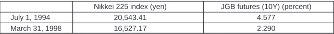
¥129.4 (9.69 percent) rise. This confirms that performance differed according to the structure of the portfolio. For reference, Appendix Figure 1 contains parities and premiums on the base dates. Table 1 shows the Nikkei 225 index and Japanese government bond futures interest rates (10 year) for the base dates.
4. Results of VaR calculation and related observations
Tables 2 and 3 contain VaR calculation results for Sub-portfolio A and Sub-portfolio B for July 1, 1994 and March 31, 1998. Both tables also contain coefficients indicat-ing the degree of contribution of each risk category to the VaR for each issue (and each sub-portfolio).
The following characteristics are observed for the calculated VaR.
Characteristics specific to Sub-portfolio A (Table 2)
(1) The results from the base date of July 1, 1994 show many individual issues for which the degree of contribution of implied volatility fluctuation in Monte Carlo simulation VaR (IV-VaR25) was roughly as high as that of share price fluctuation
(S-VaR). (In some cases, it was actually higher than S-VaR, for example, Hitachi No. 5.) What this means is that implied volatility fluctuation risk cannot be ignored even for issues with high parities and a large degree of share price-linkage. (2) The results from the base date of March 31, 1998 indicate that the degree of con-tribution of share price fluctuation (S-VaR) declined as share prices themselves declined, but for many issues the degree of contribution of implied volatility fluc-tuation (IV-VaR) remained high. What this indicates is that when share prices declined and convertible bonds began to move from being share-price-driven to interest-rate-driven,26 implied volatility was a factor impacting price fluctuation
on both base dates.
(3) Among the changes from one base date to the other was the decline in the VaR for this sub-portfolio from 4.00 percent on July 1, 1994 to 1.74 percent on March 31, 1998. The breakdown by risk category indicates that there were sub-stantial declines in the degrees of contribution of both share price fluctuation and interest rate fluctuation (S-VaR went from 4.09 percent to 2.12 percent; R-VaR from 1.13 percent to 0.42 percent). From the perspective of individual issues, the degree of contribution of implied volatility fluctuation did decline (for example,
Table 1 Share Prices and Interest Rates on Base Dates
Nikkei 225 index (yen) JGB futures (10Y) (percent) July 1, 1994 20,543.41 4.577
March 31, 1998 16,527.17 2.290
25. IV-VaR is a VaR calculated using only implied volatility as a source of risk. More specifically, it fixes the underlying asset price and interest rate at the values found on the base date and then changes only implied volatility (generating multivariate ordinary random numbers) to calculate VaR according to Monte Carlo simulation. Similarly, S-VaR changes only share prices and R-VaR only interest rates, fixing the other two risk categories to calculate VaR.
26. The decline in share prices caused parity to decline, but prices in the convertible bond market did not decline until well after share prices. Because of this, the decline in parity caused the premium to rise, which made issues more driven by interest rates.
Table 2 Results of VaR Simulation for Sub-Portfolio A Base date: July 1, 1994
Issuer No. (percent)MS-VaR (percent)S-VaR (percent)IV-VaR (percent)R-VaR VaR (percent)Uncorrelated Simple VaR(percent)
Sekisui House 15 8.13 3.85 7.39 1.63 8.49 4.54 Shin-Etsu Chemical 5 9.77 9.86 0.97 0.29 9.91 10.65 Sumitomo Bakelite 5 5.61 2.66 5.54 1.85 6.42 4.46 Japan Energy 4 4.93 3.21 3.61 1.77 5.15 4.94 Ebara 2 7.86 5.98 5.27 0.91 8.02 6.65 Hitachi 5 10.13 6.21 7.42 1.13 9.74 7.19 Toshiba 6 6.89 6.13 3.06 0.73 6.89 7.55 Sharp 11 7.25 6.53 1.88 0.37 6.81 7.32
Kyushu Matsushita Electric 3 7.41 6.94 2.49 0.90 7.43 8.03
Matsushita Electric Works 7 5.91 3.67 3.47 1.26 5.20 5.11
Dai Nippon Printing 5 7.52 6.09 5.35 1.26 8.21 7.24
Mitsui & Co. 3 6.47 6.04 3.42 1.04 7.02 6.82
Daimaru 12 9.93 7.71 7.77 1.80 11.09 7.45
Nippon Express 4 8.32 6.36 5.57 0.95 8.51 7.01
Chubu Electric Power 1 3.48 0.79 1.69 2.26 2.93 1.36
Sub-portfolio 4.00 4.09 1.69 1.13 4.57 4.76
Positive correlation VaR — 5.57 4.27 1.17 — 6.54
Base date: March 31, 1998
Issuer No. (percent)MS-VaR (percent)S-VaR IV-VaR(percent) (percent)R-VaR VaR (percent)Uncorrelated Simple VaR(percent)
Sekisui House 15 0.88 0.32 0.37 0.71 0.86 0.32 Shin-Etsu Chemical 5 10.75 11.20 1.32 0.02 11.28 12.74 Sumitomo Bakelite 5 0.15 0.01 0.01 0.15 0.15 0.11 Japan Energy 4 0.62 0.05 0.05 0.62 0.62 0.00 Ebara 2 4.40 4.08 5.12 0.59 6.58 4.14 Hitachi 5 6.85 3.87 6.21 0.46 7.34 4.74 Toshiba 6 2.96 1.77 2.93 0.41 3.45 2.29 Sharp 11 0.20 0.06 0.06 0.20 0.21 0.00
Kyushu Matsushita Electric 3 0.65 0.07 0.07 0.65 0.65 0.00
Matsushita Electric Works 7 4.68 3.85 4.77 0.25 6.14 4.30
Dai Nippon Printing 5 6.53 6.55 3.06 0.29 7.23 6.91
Mitsui & Co. 3 4.92 4.00 2.40 0.45 4.69 5.15
Daimaru 12 1.69 0.66 1.04 1.18 1.71 0.67
Nippon Express 4 6.23 4.03 5.46 0.80 6.83 4.13
Chubu Electric Power 1 0.29 0.04 0.04 0.28 0.28 0.00
Sub-portfolio 1.74 2.12 1.08 0.42 2.41 2.29
Positive correlation VaR — 3.05 2.25 0.45 — 3.43
Notes: MS-VaR is the VaR measured by Monte Carlo simulation. S-VaR is the contribution of share price fluctuation to MS-VaR. IV-VaR is the contribution of implied volatility fluctuation to MS-VaR. R-VaR is the contribution of interest rate fluctuation to MS-VaR.
Uncorrelated VaR is the VaR calculated with correlation of zero between risk categories assumed. Positive correlation VaR is the VaR calculated assuming a correlation of one between issues. For each issue (and sub-portfolio), the risk category which has the largest contribution is shaded.
Table 3 Results of VaR Simulation for Sub-Portfolio B Base date: July 1, 1994
Issuer No. (percent)MS-VaR (percent)S-VaR (percent)IV-VaR (percent)R-VaR VaR (percent)Uncorrelated Simple VaR(percent)
Sekisui House 3 6.78 2.02 6.75 2.18 7.37 2.06
Sapporo Breweries 1 10.11 1.78 9.82 2.36 10.26 1.89
Teijin 7 6.99 3.25 6.80 2.04 7.81 3.71
Asahi Chemical Industry 7 8.60 3.66 9.49 2.16 10.39 3.66
Mitsubishi Chemical 6 5.28 1.78 4.18 2.56 5.22 1.94 Nippon Oil 4 8.95 2.45 8.78 2.23 9.39 2.45 Nippon Oil 5 5.05 1.06 4.44 2.15 5.05 1.21 Mitsubishi Electric 4 6.84 2.94 5.98 1.95 6.94 3.32 NEC 6 7.01 3.65 6.21 2.11 7.51 3.94 Daiwa Securities 7 10.44 4.27 10.17 2.02 11.21 4.98 Nikko Securities 4 9.50 3.13 9.30 2.09 10.03 3.32 Nikko Securities 8 8.67 3.70 8.23 1.83 9.20 3.73 Nomura Securities 7 5.66 1.75 5.05 2.08 5.74 2.22 Mitsubishi Estate 16 8.01 2.26 7.92 2.48 8.61 2.45
All Nippon Airways 4 6.95 2.51 6.10 2.24 6.96 2.87
Sub-portfolio 3.30 1.86 2.65 2.17 3.89 1.92
Positive correlation VaR — 2.69 7.28 2.16 — 2.93
Base date: March 31, 1998
Issuer No. (percent)MS-VaR (percent)S-VaR IV-VaR(percent) (percent)R-VaR VaR (percent)Uncorrelated Simple VaR(percent)
Sekisui House 3 1.70 0.74 1.41 0.66 1.72 0.72
Sapporo Breweries 1 0.70 0.04 0.05 0.67 0.68 0.09
Teijin 7 2.08 1.43 1.71 0.67 2.33 1.38
Asahi Chemical Industry 7 1.59 0.71 1.40 0.81 1.77 1.10
Mitsubishi Chemical 6 0.75 0.18 0.21 0.70 0.75 0.21 Nippon Oil 4 1.15 0.56 0.72 0.83 1.23 0.41 Nippon Oil 5 0.66 0.39 0.39 0.33 0.65 0.30 Mitsubishi Electric 4 1.44 0.34 1.22 0.87 1.54 0.65 NEC 6 2.89 1.68 2.49 0.62 3.06 1.79 Daiwa Securities 7 1.12 0.43 0.70 0.72 1.09 0.40 Nikko Securities 4 0.58 0.07 0.10 0.61 0.62 0.10 Nikko Securities 8 0.34 0.00 0.00 0.34 0.34 0.00 Nomura Securities 7 0.35 0.00 0.00 0.34 0.34 0.07 Mitsubishi Estate 16 3.01 1.74 2.70 0.77 3.30 1.69
All Nippon Airways 4 0.80 0.00 0.00 0.86 0.86 0.01
Sub-portfolio 0.76 0.34 0.52 0.64 0.89 0.36
Positive correlation VaR — 0.56 0.88 0.65 — 0.60
Notes: MS-VaR is the VaR measured by Monte Carlo simulation. S-VaR is the contribution of share price fluctuation to MS-VaR. IV-VaR is the contribution of implied volatility fluctuation to MS-VaR. R-VaR is the contribution of interest rate fluctuation to MS-VaR.
Uncorrelated VaR is the VaR calculated with correlation of zero between risk categories assumed. Positive correlation VaR is the VaR calculated assuming a correlation of one between issues. For each issue (and sub-portfolio), the risk category which has the largest contribution is shaded.
Sekisui House No. 15 saw a decline from 7.39 percent to 0.37 percent), but when viewed from the perspective of the sub-portfolio, the dispersion effect prevented the impact from being felt in individual issues (the sub-portfolio as a whole went from 1.69 percent to 1.08 percent).
Characteristics specific to Sub-portfolio B (Table 3)
(1) The results from the base date of July 1, 1994 show that implied volatility fluctu-ation had a higher degree of contribution (IV-VaR) than share price fluctufluctu-ation or interest rate fluctuation (S-VaR, R-VaR). This indicates the importance of managing implied volatility risks.
(2) The results from the base date of March 31, 1998 show that for many issues, S-VaR declined to below 1.00 percent, so that the major risk factors became implied volatility and interest rates. Implied volatility tended to be a particularly important risk factor for issues with comparatively long terms to maturity.
(3) Among the changes from one base date to the other for all issues were declines in the values for Monte Carlo simulation VaR (the sub-portfolio went from 3.30 percent to 0.76 percent), S-VaR (from 1.86 percent to 0.34 percent), IV-VaR (from 2.65 percent to 0.52 percent), and R-VaR (from 2.17 percent to 0.64 percent).
Characteristics common to both sub-portfolios (tables 2 and 3)
(1) To observe the influence of different risk categories on each other, we calculated VaR with a correlation of zero between risk categories (uncorrelated VaR27), which
we found to be higher than Monte Carlo simulation VaR for both sub-portfolios on both base dates. (For example, in Table 2, the sub-portfolio Monte Carlo simu-lation VaR on July 1, 1994 was 4.00 percent, while the uncorrelated VaR was 4.57 percent.) This relationship was also commonly observed for individual issues, and what it indicates is that the correlation between different risk categories (the negative correlation between share price fluctuation and implied volatility fluctuation,28 and the positive correlation between share price fluctuation and
interest rate fluctuation) had the effect of reducing risk values of the whole. (2) To observe the influence of different issues on each other, we calculated VaR
with the correlation between issues set at one (positive correlation VaR29). We
found that within risk categories, the positive correlation grows weaker in a category for interest rates, share prices, and implied volatility, in that order (the correlation is smaller the larger the difference between the positive correlation VaR and the sub-portfolio VaR). Note that implied volatility fluctuation is highly
27. Below is the uncorrelated VaR formula for issue i(or for a sub-portfolio): (Uncorrelated VaRi)2= (S•VaRi)2+ (IV•VaRi)2+ (R•VaRi)2.
28. See Section III.A for a statistical analysis of the negative correlation between share prices and implied volatility. 29. A positive correlation VaR is the VaR found when share price fluctuations corresponding to the 99th percentile
of each issue occurred simultaneously. In other words, we can express the 99th percentile value for share price fluctuation for issue ibecause of fluctuation in risk category jas ∆Vi(99%)j. This allows us to calculate a positive
correlation VaR for risk category jas follows: Positive correlation VaRj= ∑∆Vi(99%)j/∑Vi,0,
i i
dependent on individual issue factors, which means that there is little correlation between issues.
These findings have three implications for Monte Carlo simulation VaR calculations.
(1) There are cases in which implied volatility is the major factor in market risk (as on the July 1, 1994 base date for Sub-portfolio B).
(2) Implied volatility risk is present even when parity is low and there is little link-age to share prices. Attempts to value only interest rate risk may understate the risks involved (as on the March 31, 1998 base date for Sub-portfolio B). (3) The VaR for implied volatility fluctuation provides fairly large risk values for
individual issues, but the use of portfolios has the effect of reducing this risk. We also performed calculations under the simple method, which considers only share price risk. Below is a summary of how the characteristics of these results differ for those from the Monte Carlo simulation.
First, at the individual issue level, the risk values found with the simple method were not more conservative than those with the Monte Carlo simulation except for a few issues with an extremely high degree of share price-linkage (issues with deltas of 0.8 or more and vegas of 0.7 or less).
At the portfolio level, the simple method produced more conservative VaRs than the Monte Carlo simulation for Sub-portfolio A on both base dates. These results imply the following about the simple method:
(1) The simple method is an effective tool for managing individual issues as long as their deltas are high (for example, over 0.8) and their vegas relatively low (under 0.7). For other issues, however, the implied volatility fluctuation risk cannot be ignored, so it will be necessary to estimate the risks associated with implied volatility fluctuation (and also the risks associated with interest rate fluctuation) separately.
(2) The simple method may be an effective tool for portfolio-level management even if the simple method only considers delta risk. This is because effects of the risks associated with implied volatility fluctuation are relatively small at the portfolio level thanks to the issue diversification effect.
5. Analysis of risk factors in convertible bonds
This subsection analyzes the degree of sensitivity that individual issues have to share prices, implied volatility, and interest rates. In the preceding analysis of market risk, we saw that the three risk categories changed with some degree of correlation. In this analysis, we will focus on implied volatility in particular.
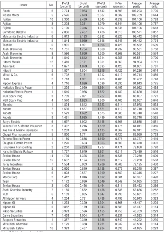
Table 4 contains price volatility (P-Vol) for individual issues (standard deviation of the weekly rate of change for market prices observed for the period January 7, 1994 through December 1, 1995). We have also included the degree of contribution of individual risk categories (share prices, implied volatility, and interest rates) on price volatility (noted as S-Vol, IV-Vol, and R-Vol, respectively).
Table 4 lists issues in order of average parity for the observation period, with the highest parities at the top. Note that the higher the convertible bond’s parity (and therefore its delta), the higher its price volatility (P-Vol). Turning to price fluctuation factors, we can see that below an average parity of 80, there is an increase in the
Table 4 Factor Analysis of Price Fluctuation:
Observation Period January 7, 1994–December 1, 1995
Issuer No. (percent)P-Vol (percent)S-Vol (percent)IV-Vol (percent)R-Vol Averageparity Averagedelta
Ricoh 6 2.774 2.933 1.642 0.303 107.293 0.720 Nissan Motor 5 2.576 2.673 2.387 0.382 102.769 0.644 Fujitsu 10 2.300 2.469 1.343 0.332 101.106 0.728 Fujitsu 8 2.208 2.361 1.079 0.344 101.106 0.767 Fujitsu 9 2.100 2.376 1.007 0.346 101.106 0.618 Sumitomo Bakelite 6 2.036 2.457 1.426 0.313 100.571 0.857 Matsushita Electric Industrial 6 2.012 2.183 0.882 0.325 98.442 0.840 Matsushita Electric Industrial 5 1.844 1.959 0.896 0.345 98.442 0.774
Toshiba 6 1.901 1.921 1.996 0.426 96.562 0.599 Asahi Breweries 10 1.751 1.764 1.369 0.237 95.581 0.750 Asahi Breweries 9 1.596 1.666 1.300 0.269 95.581 0.574 Asahi Breweries 8 1.540 1.642 1.314 0.255 95.581 0.700 Hitachi Metals 12 1.410 2.171 1.351 0.363 94.994 0.711 Aisin Seiki 7 1.677 1.879 1.393 0.420 94.961 0.781 Hitachi 5 1.857 1.804 1.816 0.425 94.236 0.614
Mitsui & Co. 6 1.702 2.151 1.312 0.419 93.714 0.856
Ebara 2 1.713 1.961 0.405 0.405 93.462 0.748
Nippon Express 4 1.716 1.896 1.596 0.395 91.643 0.775 Hokkaido Electric Power 1 1.229 0.960 1.664 0.495 91.062 0.468 Hokuriku Electric Power 1 1.540 0.936 1.622 0.480 89.620 0.518 NGK Spark Plug 3 1.709 2.021 2.727 0.400 88.057 0.721 NGK Spark Plug 4 1.570 1.833 1.600 0.405 88.057 0.646 Shimizu 1 1.824 1.842 2.323 0.514 87.978 0.538 Kubota 7 1.536 1.567 1.571 0.412 86.740 0.609 Kubota 9 1.529 1.692 1.573 0.383 86.740 0.540 Kubota 8 1.481 1.625 1.499 0.407 86.740 0.525 Sanyo Electric 6 1.697 1.902 2.145 0.566 86.665 0.551 Yasuda Fire & Marine Insurance 3 1.407 1.216 1.529 0.475 84.011 0.385 Koa Fire & Marine Insurance 3 1.203 0.978 1.113 0.367 82.911 0.285 Chugai Pharmaceutical 5 1.800 1.741 1.757 0.420 82.069 0.753 Tohoku Electric Power 1 1.180 0.886 1.590 0.575 81.727 0.419 Chugoku Electric Power 1 1.270 0.603 1.363 0.600 80.470 0.391 Fukuyama Transporting 2 2.250 2.223 1.727 0.471 79.858 0.720 Hanshin Electric Railway 9 1.727 1.649 1.801 0.511 79.489 0.516 Sekisui House 14 1.795 1.325 1.934 0.538 79.280 0.509 Sekisui House 15 1.697 1.124 1.699 0.517 79.280 0.563 Toray Industries 7 1.534 0.963 1.709 0.706 72.195 0.430 Sekisui House 5 2.020 0.810 2.158 0.676 69.345 0.387 Sekisui House 6 1.028 0.537 1.010 0.559 69.345 0.227 Maeda Corp. 2 1.412 1.046 1.692 0.681 68.377 0.420 Teijin 7 1.172 0.836 1.349 0.849 57.085 0.282 Sekisui House 3 1.409 0.466 1.464 0.811 56.463 0.266 Asahi Chemical Industry 7 1.185 0.582 1.458 0.836 53.666 0.282
NEC 6 1.109 0.835 1.047 0.790 53.631 0.267
All Nippon Airways 4 1.254 0.731 1.488 0.796 50.943 0.323 Nippon Oil 4 1.278 0.390 1.304 0.868 48.417 0.229 Nippon Oil 5 0.862 0.179 1.043 0.683 48.417 0.114 Nikko Securities 4 0.973 0.596 1.155 0.756 46.769 0.229 Daiwa Securities 7 1.459 1.004 1.471 0.837 44.523 0.314 Sapporo Breweries 1 1.357 0.349 1.356 0.842 44.292 0.230 Mitsubishi Chemical 6 1.179 0.388 1.281 0.932 43.568 0.144 Mitsubishi Estate 16 1.323 0.437 1.284 0.898 41.895 0.223 Notes: P-Vol is share price volatility.
S-Vol is the contribution of share price fluctuation to P-Vol. IV-Vol is the contribution of implied volatility fluctuation to P-Vol. R-Vol is the contribution of interest rate fluctuation to P-Vol.
degree of contribution to risk of implied volatility (IV-Vol30), which indicates that
implied volatility fluctuation becomes the main factor in convertible bond price fluctuation. While the degree of contribution of share price fluctuation (S-Vol) tends to decline the lower the average delta, the degree of contribution of implied volatility fluctuation (IV-Vol) is generally high and stable for issues with low average deltas and average parities.
Table 5 contains the results of a similar analysis performed for the 1996–97 period. This period saw further declines in share prices, which made issues even more strongly linked to interest rates. But even under these conditions, implied volatility fluctuation continued to be the main factor in convertible bond price fluctuation.
Table 5 Factor Analysis of Price Fluctuation:
Observation Period May 1, 1996–November 21, 1997
Issuer No. (percent)P-Vol (percent)S-Vol (percent)IV-Vol (percent)R-Vol Averageparity Averagedelta Hokkaido Electric Power 1 0.898 0.285 1.009 0.376 81.922 0.176 Hokuriku Electric Power 1 1.080 0.449 1.167 0.365 81.653 0.250 Toray Industries 7 0.543 0.824 0.927 0.354 79.553 0.300 Chugoku Electric Power 1 0.422 0.266 0.588 0.358 73.200 0.151 Tohoku Electric Power 1 0.450 0.270 0.599 0.369 70.117 0.143 Sekisui House 5 0.930 0.377 0.904 0.449 67.563 0.108 Sekisui House 6 0.472 0.161 0.445 0.261 67.563 0.049 NEC 6 0.881 0.573 0.728 0.390 66.873 0.156 Teijin 7 0.622 0.282 0.627 0.443 57.573 0.085 Mitsubishi Estate 16 0.664 0.368 0.579 0.488 57.212 0.098 Sekisui House 3 0.471 0.157 0.487 0.444 55.012 0.052 Asahi Chemical Industry 7 0.628 0.219 0.705 0.481 51.477 0.097 Sapporo Breweries 1 0.462 0.179 0.560 0.422 45.722 0.100 Nippon Oil 4 0.547 0.230 0.630 0.481 44.860 0.104 Nippon Oil 5 0.276 0.109 0.333 0.277 44.860 0.048 All Nippon Airways 4 0.635 0.235 0.700 0.476 42.441 0.106 Nikko Securities 4 0.663 0.239 0.517 0.371 37.401 0.085 Mitsubishi Chemical 6 0.502 0.199 0.495 0.442 35.384 0.087 Daiwa Securities 7 0.685 0.225 0.655 0.450 33.891 0.121 Note: For each issue, the risk category which has the largest contribution is shaded.
At present, the convertible bond market contains a high percentage of issues with conversion prices below share prices, and in situations like this it is particularly important to manage implied volatility, which is one of the risk parameters peculiar to convertible bonds.
Our Monte Carlo simulation (VaR calculation) did not explicitly consider the influence of time on convertible bond prices. Most convertible bonds are low-coupon bonds, and because of this the price of their bond component tends to be under par. The value of the bond component rises over time31 (all else being equal) 30. IV-Vol is the price volatility of the convertible bond when only implied volatility fluctuation is taken into account. In other words, a binomial tree model of the theoretical price of the convertible bond is created using the current value only for implied volatility and previous values for other price fluctuation factors (underlying asset prices, interest rates). The rate of return from the theoretical price is then used to calculate a weekly price volatility. Similarly, S-Vol and R-Vol express price volatility for theoretical prices calculated when only share prices and interest rates (respectively) are allowed to change and all other price fluctuation factors are kept the same. 31. It is conceivable that there would be convertible bonds over par when interest rates are low, and in this case the
and gradually moves closer to par, but as this is happening, the time value of the conversion option wanes because the term to maturity declines. Therefore, the value of the convertible bond will decline over time when the bond is highly linked to share prices, but will tend to rise over time when it is highly linked to interest rates. We considered these effects to be predictable and therefore excluded them from our definition of risk in this simulation, though it would be possible to include them. Suffice it to underscore here the need to pay particularly close attention to declines in time value for highly share price-driven portfolios.
III. Empirical Analysis of Japanese Convertible Bond Market
In this chapter, we use the binomial tree pricing model discussed in Chapter II to transform market price data for convertible bonds into implied volatility data and then perform a number of regression analyses and analyze market characteristics.
During the late 1980s, Japanese companies reduced the weight of bank borrow-ings in their fund-raising in favor of issues of equity-linked bonds, primarily convertible bonds and bonds with warrants. The traditional explanation for this behavior has been that “equity-linked bonds were a cheaper means of fund-raising than either bank borrowings or straight bonds.” Cheaper in this context means that coupons were lower than they would have been for bank borrowings or straight bonds. However, the cost to issuers from convertible bond fund-raising is not just the coupon but the value of the options sold in order to reduce that coupon, since the issuer receives a premium from investors for the options it sells, which effectively helps it to reduce costs. In other words, the higher the issuing conditions with respect to the implied volatility of the conversion option, the more advantageous this method is to the issuer.
As this example illustrates, an analysis of implied volatility is essential to under-standing the nature of the convertible bond market. Our analysis in the preceding chapter indicated that implied volatility was strong for individual convertible bond issues (but with very little correlation among issues). Nonetheless, it has been fairly rare in traditional analyses of the convertible bond market to delve into detailed analysis of implied volatility data at the individual issue level. In this chapter, we use the time-series implied volatility data calculated from the binomial tree model to observe the workings of the convertible bond market.
Our analysis covers weekly data on convertible bonds issued in 1987 and 1994 with a rating of at least BBB and an issue amount of at least ¥20 billion. We will refer to Appendix Figure 2 and Appendix Figure 3 in discussing implied volatility for some of the issues covered in this analysis.
A. Linkage between the Convertible Bond Market and the Stock Market
In Section II.C, we observed that for most issues there was a negative correlation between share price and implied volatility, the risk parameters of convertible bonds. In this section, we see statistical verification of the significance of this correlation.
We use a regression model to accomplish this.32
IVi,t+1– IVi,t= ai+bi(SPi,t+1– SPi,t) + εi,t, (1)
where
iis the issue,
tis the weeks elapsed, t= 0, 1, 2, . . . ,
SPis the share price.
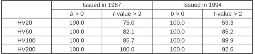
When coefficient b is negative and the t-value (absolute) is large, there will be a strong negative correlation between share price fluctuation and implied volatility fluctuation. Appendix Table 2 contains regression results for individual issues, with the overall trends summarized in Table 6.
Table 6 Summary of Results for Coefficient b on Regression Model (1)
—Ratio of issues with negative coefficient b and significant t -value to all sample issues Percent
Issued in 1987 Issued in 1994 b < 0 t -value < –2 b < 0 t -value < –2 100.0 85.7 100.0 96.3
These results find a negative value for coefficientb for all issues and at-value (absolute) in excess of two for most issues, which confirms that there is a significant negative correlation between share price fluctuation and implied volatility fluctuation.33
Let us now examine two hypotheses regarding this negative correlation.
(1) This is a phenomenon that is commonly seen between share prices and the implied volatility of options with shares as underlying assets, and is not something peculiar to the convertible bond market.
(2) This is a phenomenon that is peculiar to the convertible bond market, and it happens because convertible bond prices respond sluggishly to changes in the price of their underlying shares. For example, when the share price rises (or falls), convertible bond prices do not incorporate the move, which causes a decline (rise) in nominal implied volatility.
We tested the first hypothesis with a similar analysis of options on the Nikkei 225 index, as shown in Table 7. We did not find significance for either coefficient bor the
t-value for any observation period and indeed could find no negative correlation like that seen for the convertible bond.
These findings make it difficult to conclude that it is common to have a negative correlation between underlying asset price fluctuation and implied volatility fluctuation. We have therefore rejected hypothesis (1).
32. All of the models in this paper, including this one, are time-series data analysis models for individual issues. As an alternative to these models, panel data models could be used. When performing the analysis for this paper, we began by testing panel data analysis, but F-tests forced us to reject panel data handling and select analysis of individual issues. Because of this, all of the analysis that follows is time-series data analysis for individual issues. 33. It is conceivable that a positive correlation could similarly be demonstrated for implied volatility fluctuation and
We do not directly test hypothesis (2) in this paper, though this also means that we cannot reject the possibility that there are other factors in the convertible bond market that would cause a negative correlation besides those in hypothesis (2). We would, however, draw the reader’s attention to prior research34 that points to a
time lag between changes in share prices and changes in convertible bond prices. Compared to the Nikkei 225 index market, the convertible bond market lacks liquidity and effective hedge functions (futures, lending market). It may be, there-fore, that price formation in this market is unable to fully reflect price movements in the stock market that underlies it. Nonetheless, the fact that implied volatility is influenced by sluggish price response is one of the characteristics of the convertible bond market.
B. Weak Arbitrage in the Convertible Bond Market
In this section, we use historical volatility to investigate the fluctuation characteristics of implied volatility in the secondary market for convertible bonds.
Implied volatility evaluation is essential to investment studies of option-style instruments, as we have already demonstrated. One benchmark to be used in deter-mining whether implied volatility is relatively high or relatively low is the historical volatility of the underlying assets.35 We will therefore consider the relationship
between the implied volatility of options on the Nikkei 225 index and the historical volatility of the Nikkei 225 index.
Figure 3 plots implied volatility for the nearest contract month for options on the Nikkei 225 index and 10-day historical volatility (HV10) for the Nikkei 225 index.
34. See Nakamura and Suzuki (1997).
35. We must emphasize that historical volatility is data on the historical fluctuation of the underlying assets and does not directly predict future fluctuation.
Table 7 Results for Regression Model (1) Applied to the Nikkei 225 Index
Period a t -value b t -value R–2
1994–95 –0.0768 –0.2608 0.0007 1.2249 0.0049 1995–96 –0.0677 –0.1814 0.0007 0.8942 –0.0020 1996–97 0.0765 0.2125 –0.0001 –0.1581 –0.0097 0 10 20 30 40 50 60 70 IV HV10 Volatility (percent) Mar. 1993 1993Sep. Mar. 1994 Sep. 1994 Mar. 1995 Sep. 1995 Mar. 1996 Sep. 1996 Mar. 1997 Sep. 1997 Mar. 1998 Figure 3 Movement of Implied Volatility for Options on the Nikkei 225 Index and