Outline 2. 1 Turing Machines. 2 Coding and Universality. 3 The Busy Beaver Problem. 4 Wolfram Prize. 5 Church-Turing Thesis.

CDM

Turing Machines

Klaus Sutner Carnegie Mellon University

3-turing-mach

2015/8/30 19:46

Outline

1 _{Turing Machines}

2 _{Coding and Universality}

3 The Busy Beaver Problem

4 Wolfram Prize

5 _{Church-Turing Thesis}

Intuitive Computability

How can we capture the intuitive notion of computability?

Historically, the first notions of computability suggested around 1930 were

G¨odel-Herbrand general recursive functions, and Church’sλ-calculus.

G¨odel was not entirely convinced that these proposals properly capture computability.

Alan Turing

Soundness and Completeness

We need to identify a formal notion of computability that

arguably does not go beyond what a human computor could do (in principle), and

arguably captures everything a human computor can do.

Note that qualifier “arguably,” there won’t be a theorem.

Turing’s Machines

Basic Idea: Observe the computor. We all agree that mathematicians compute (among other things such as drinking coffee or proving theorems).

So we could try to define an abstract machine that can perform any calculation whatsoever that could be performed in principle by a mathematician, and only those. To this end we need to formalize what a computor is doing.

Mathematicians can always write down their calculations on paper. This amounts simply to bookkeeping of all intermediate results.

We need to formalize what can be written down and the rules that control the process of writing things down.

Also note that Turing had terrible handwriting, he was always interested in typewriters. His machines are, in a sense, just glorified typewriters.

The Abstraction

Mathematicians use two-dimensional notation, but could all be flattened out into one-dimensional notation.

Only finitely many symbols are allowed.

Can think of having a strip of paper subdivided into cells, each cell containing exactly one symbol (possibly the blank symbol).

12345 * 6789 74070 86415 98760 111105 83810205 is flattened out into the linear string

12345 * 6789 74070 86415 98760 111105 = 83810205

Digression

Flattening out notation is standard when dealing with keyboard input. Instead of Z1 0 1 2 +x2dx= arctan(_√1 2) √ 2

one has to deal with something like

Integrate[1/(2 + x^2), {x,0,1}] ==> ArcTan[1/Sqrt[2]]/Sqrt[2]

The Rules

The input is written on an otherwise empty tape.

The computor’s mind has finitely many possible states and is always in one particular of these states.

At each step, the computor focuses on one particular cell, the current cell. The computor inspects the current cell and takes action depending on his own state of mind and the symbol in the cell.

• She may overwrite the symbol in the current cell.

• She may shift attention to the cell on the left or right.

• She may switch into a new state of mind.

Initially, she is in state “start” and looks at the first empty cell to the left of the input.

The computor keeps doing this until a state of mind “finished” is reached.

What is written on the tape at this point constitutes the result of the computation.

Justification

These assumptions are quite robust.

It would take the computor infinitely long to learn the meaning of infinitely many symbols.

Likewise, the mind can assume only finitely many configurations (quantum physics, digital physics).

A human mind cannot pay attention to infinitely many symbols. But finitely many symbols is the same as, say, 2.

Likewise a step cannot depend on infinitely many symbols. But using finitely many symbols is the same as just using one.

All but finitely many cells will always contain a special blank symbol. Otherwise someone would already have had to spend an infinite amount of time writing down the initial tape contents.

Finite Tapes

It should be noted that the last condition is a bit harsh.

It is certainly justified to insist on a very simple initial tape inscription, but all blanks on either side of the input pushes things a bit.

For example, an inscription of the form

. . .000010000100001x1x2. . . xn−1xn1000010000100001. . . is surely harmless.

For Turing machines, this makes no difference whatsoever, but there are other models of computation such as cellular automata where the more general starting configurations are of great interest.

A Turing Machine

a

b

a

a

c

a

b

a

work tape

read/write head

The Pieces

Atape: a bi-infinite strip of paper, subdivided intocells. Each cell contains a single letter; all but finitely many contain just a blank. So we have atape inscription.

Aread/write headthat is positioned at a particular cell. That head can move left and right.

Afinite state controlthat directs the head: symbols are read and written, the head is moved around and the internal state of the FSC changes.

Formalization

alphabetΣ: finite set of allowed symbols, special blank symbol ∈Σ state setQ: finite set of possible mind configurations

δ:Q×Σ→Q×Σ× {−1,0,1}:transition function a specialinitial stateq0∈Q

a specialhalting stateqH∈Q.

Definition

ATuring machineis a structureM=hQ,Σ, δ, q0, qHi.

Example: Successor Function

Tape alphabetΣ ={,1}

StatesQ={0,1,2,3}

Initial stateq0= 0, final stateqH= 3.

The transition functionδis given be the following table: p σ δ(p, σ) 0 1 +1 1 2 1 0 1 1 1 1 1 2 3 0 2 1 2 1 −1

No other transitions are needed.

Simulation

It is not hard to write a program that simulates a Turing machine. Hence, do some computational experiments on these machines. The following visualization method is sometimes useful to understand behavior of small Turing machines. In the pictures:

The tape is represented by a row of colored squares.

Time flows from top to bottom (usually; sometimes from left to right). The position of the tape head is indicated by a black frame around a square.

The rightmost column indicates the state of the machine.

Sample Run

Addition

We are using unary notation,nis represented by n7→111_{| {z }}. . .11

n+1

Hence we have to erase two 1’s at the end:

0 1 1 1 2 1 1 1 1 1 1 1 2 3 −1 2 1 2 1 1 3 1 4 −1 4 1 5 −1 5 6 0 5 1 5 1 −1

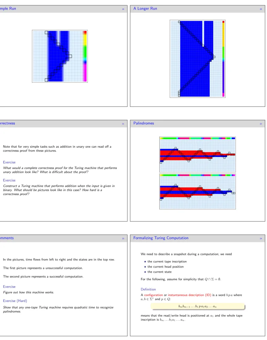
Sample Run

A Longer Run

Correctness

Note that for very simple tasks such as addition in unary one can read off a correctness proof from these pictures.

Exercise

What would a complete correctness proof for the Turing machine that performs unary addition look like? What is difficult about the proof?

Exercise

Construct a Turing machine that performs addition when the input is given in binary. What should be pictures look like in this case? How hard is a correctness proof?

Palindromes

Comments

In the pictures, time flows from left to right and the states are in the top row.

The first picture represents a unsuccessful computation.

The second picture represents a successful computation.

Exercise

Figure out how this machine works.

Exercise (Hard)

Show that any one-tape Turing machine requires quadratic time to recognize palindromes.

Formalizing Turing Computation

We need to describe a snapshot during a computation; we need the current tape inscription

the current head position the current state

For the following, assume for simplicity thatQ∩Σ =∅.

Definition

Aconfigurationorinstantaneous description (ID)is a wordb p awhere a, b∈Σ?_andp∈Q:

bmbm−1. . . b1p a1a2. . . an

means that the read/write head is positioned ata1and the whole tape

The Step Relation

We need to explain the one-step relation bpa M

1

b0qa0

Letδ(p, a1) = (q, c,∆)Then the “next configuration” is defined by

bm. . . q b1ca2. . . an ∆ =−1

bm. . .b1q ca2. . . an ∆ = 0

bm. . .b1c q a2. . . an ∆ = +1

Here we assume thataandbare non-empty, otherwise we can setb1=a1= .

Many Steps

As always, we extend the “one-step” relation to multiple steps by iteration:

C M 1 C0_{: one step} C M t C0_{: exactlytsteps}

C M C0: any finite number of steps

The last notion is problematic: there is no bound on the number of steps.

Input and Output

Given any inputx1, x2, . . . , xn∈Σtheinitial configurationis

Cx=q0 x1x2. . . xn Afinal configurationis of the form

CH

y =qH y1y2. . . ym

For input we have chosen to place the head at the last blank to the left of the input symbol, there are lots of other possibilities (e.g,q0x1. . . xn).

Also, we require our machines to erase the tape (except for the output) and return the tape head to the initial position before halting; nothing important changes if we drop this condition.

Computations

IfCx M CHy theny=y1, y2, . . . , ymis the output of the computation of machineMon inputx.

Mcomputesf:Nk_,

→Nif, for allx∈Nk_,

Iffis defined onxthenCx M CyHandf(x) =y.

Iffis undefined onxthen the computation ofMonxdoes not halt.

Herexis ak-tuple of natural numbers andx∈Σ?_{is the corresponding} tape-inscription.

Halting

Note that a Turing machine may very well fail to reach the halting stateqH during a computation.

For example, the machine could ignore its input and just move the head to right at each step.

Or it could go into an “infinite loop” where the same sequence of configurations repeats over and over again.

As it turns out, this is not a bug but a feature: we will see shortly that failure to halt is a problem that cannot be eliminated.

There are restricted types of Turing machines that a guaranteed to halt on all inputs, but unfortunately they do not capture the full notion of computability.

Computable Functions

Definition

A functionf:Nk_{,→Nis(Turing) computableif there is a Turing machineM} that computesf.

Note that these functions are potentially partial: on any particular input the TM may fail to halt. In fact, the machine may fail to halt on all inputs.

Historically these functions are also calledpartial recursive functions. The ones that are in addition total are called(total) recursive functions.

Relations

We can use thecharacteristic functionof a relationR

charR(x) =

1 x∈R

0 otherwise. to translate relations into functions.

Definition

A relation is(Turing) decidableif its characteristic function is Turing computable.

Historically these relations are also calledrecursive relations.

Semidecidable Relations

Since Turing machines may fail to halt one and use halting to characterize a class of relations.

Definition

A relationRis(Turing) semidecidableif there is a Turing machineMthat halts precisely on allxsuch thatR(x).

We will see shortly that a relationRis decidable iffRand its complement are both semidecidable.

Semidecidable sets are also calledrecursively enumerable (r.e.).

Turing Computability and Robustness

So we have a notion of a function being computable and a relation being decidable (or semidecidable).

These notions donotchange if we modify our definitions slightly: one-way infinite tapes

multiple tapes multiple heads

different input/output conventions

Note that without this kind of robustness our model would be essentially useless.

Input/Output Tapes

M

1

0

1

0

0

a

b

a

a

c

a

b

a

0

1

1

1

Input/Output Tapes

In this model, the

input tape is read-only, one-way infinite

output tape is write-only, one-way infinite

work tape is read/write, two-way infinite

As we will, see this is just the right model for space complexity.

The Important Ideas

We can specify a model of computation by defining

a spaceCof possible configurations (snapshots), a “next configuration” relation,

an input and output convention.

The details vary, but it’s always the same pattern.

Details about input/output conventions become really important in low complexity classes; higher up they are all interchangeable.

Models of Computation

C

Nk

N

C _C0

The number-theoretic scenario (input and output are natural numbers).

Models of Computation, II

C

C _C0

Σ∗ _Σ∗

The string scenario (input and output are words over some alphabet).

Exercises

Exercise

Explain how a multi-tape TM can be simulated by a single-tape TM.

Exercise

Determine how long it takes to recognize palindromes on two tapes versus one tape.

Exercise

Determine the general slow-down caused by switching from two tapes to one.

Exercise

Show that it does not matter whether the tape head is required to return to the standard left position at the end of a computation.

Turing Machines

2 Coding and Universality

The Busy Beaver Problem

Wolfram Prize

Church-Turing Thesis

TMs and Data Structures

Since Turing machines operate only on strings it is not entirely clear how powerful they are, compared to, say,Cprograms.

For example, could one concoct a TM that computes shortest paths in a graph?

The key issue is that we need to code the graph as a string. Plus all other needed data structures: lists, trees, matrices, . . .

This is not particularly difficult, but it is worth spelling out the details once and for all. In fact, we will not use strings but an more elementary setting: natural numbers (this approach is more interesting in the context of provability and systems of arithmetic).

Leopold Kronecker

Die ganzen Zahlen hat der liebe Gott gemacht, alles andere ist Menschenwerk.

“Dear god” made the integers, everything else is the work of men.

Sequence Numbers

We would like to express a sequencea1, a2, . . . , anof natural numbers as a single numberha1, a2, . . . , ani. So we need acodingfunction, a polyadic map of the form

h.i:N∗_→N

and adecoding functionthat extracts the components of a coded sequence

dec:N×N→N

so that

ai=dec(ha0, a1, a2, . . . , an−1i, i)

fori= 0, . . . , n−1.

Length

Note that dec(x, i)need not be defined wheniis too large or whenxis not of the formha0, a1, a2, . . . , an−1i.

One usually insists that the function is total and that there is alength function len(ha0, a1, a2, . . . , an−1i) =n

The numbers that appear as codes of sequences are calledsequence numbers.

Exercise

Show how to check if a number is a sequence number givendecandlen.

Pairs

The first step is to select apairing function, an injective mapN×N→N. There are many possibilities, here is a particularly simple choice:

π(x, y) = 2x_{(2y+ 1)} So

π(5,27) = 1760 = 110111000002

In Binary

Note that the binary expansion ofπ(x, y)looks like so:

ykyk−1. . . y01 00_{| {z }}. . .0

x

whereykyk−1. . . y0is the binary expansion ofywithykbeing the most significant digit.

This makes it easy to find the correspondingunpairing functions: x=π1(π(x, y)) y=π2(π(x, y)).

Extending to Sequences

hnili= 0

ha1, . . . , ani=π(a1,ha2, . . . , ani) Here are some sequence numbers for this particular coding function:

h10i= 1024 h0,0,0i= 7 h1,2,3,4,5i= 532754

That’s It!

We can now code any discrete structure as an integer by expressing it as a nested list of natural numbers, and then applying the coding function. For example, the so-called Petersen graph on the left is given by the nested list on the right.

((1,3),(1,4),(2,4),(2,5),(3,5), (6,7),(7,8),(8,9),(9,10),(6,10),

Not So Fast

Of course, we also need to be able to operate on sequence numbers.

Exercise

Construct a TM that computes the length of a sequence, given the code number as input.

Exercise

Construct a TM that computes the two unpairing functionsx=π1(π(x, y))

andy=π2(π(x, y))

Exercise

Construct a TM that implements the join of two lists given as sequence numbers.

Coding TMs

A Turing machine is essentially an×5table of numbers: The transition function has the form

δ:Q×Σ→Q×Σ×∆

and we can identify the set of statesQ, the alphabetΣand the displacement with natural numbers.

We can further assume without loss of generality that1∈Qis the initial state and, forQ={1,2, . . . , n}, thatnis the halting state.

But the table can be expressed by a single number using our coding machinery. We will writehMi for the number associated with TMM.

Universal Turing Machines

The fact that we can code a Turing machine as an integer combined with the observation that Turing machine naturally can compute on integers has an interesting consequence:

We can build a Turing machineUthat takes as input 2 numbers eandx, interpretseas the code number of a Turing machine M, and then executesMon inputx. Uwill halt oneandxiff Mhalts onx; moreover,Uwill return the same output in this case.

Any such machineUis called auniversal Turing machine.

The details of the construction ofUare very tedious, but it’s “clear” that this can be done.

Comments

IfUis given a numbereas input that fails to code a Turing machine we assume thatUfails to halt.

Clearly the argument also works for Turing machines with multiple inputs (which we can either keep separate or code into a single input).

Note thatUis by no means uniquely determined, there are lots and lots of choices.

The simulation by a universal TM is even efficient in the sense that the computation ofUwon’t take much longer than the computation ofM. A very interesting question is how large a universal Turing machine needs to be. Amazingly, there is a 2-state, 5-symbol UTM (see the lecture on cellular automata).

Enumerating Computable Functions

Fix some universal Turing machineU. Each TMMtranslates into an integer e=hMi, theindexforM.

Similarly we can think ofeas describing a particular computable function, often written

ϕe or {e}

Hence,({e})eis a complete listing of all computable functions. We won’t deal with arity issues here, they are purely technical.

Convergence and Divergence

When dealing with partial recursive functions it is convenient to have some shorthand notation for convergence and divergence:

{e}(x)↓ versus {e}(x)↑

Similarly one writes

{e}(x)'y

to mean that the left hand side converges with outputy, or both sides are undefined.

Partial versus Total

It might be tempting to think of partial recursive functions as total recursive functions restricted to some smaller domain of definition. Tempting, but very wrong.

Proposition

There is a partial recursive functiongthat is not the restriction of any total recursive function. Proof. Let g(e) = ( {e}(e) + 1 if{e}(e)↓, ↑ otherwise.

It is easy to see thatgcannot be of the formg'fDfor any total recursive functionf.

2

The Halting Problem

Problem: Halting Problem

Instance: An indexe, an inputx. Question: Does{e}(x)converge?

Theorem

The Halting Problem is undecidable.

Proof. Suppose otherwise and define a functiongby

g(e) = (

{e}(e) + 1 if{e}(e)↓,

0 otherwise.

Thengis computable, sog' {e}for somee. Contradiction via inpute. 2

Nota Bene

A definition of the form

g(x) = (

f(x) x∈A,

↑ otherwise.

wherefis computable andAis semidecidable produces a computable function. But

g(x) = (

f1(x) x∈A,

f2(x) otherwise.

does not in general. It is OK whenAis decidable, though.

Turing Machines

Coding and Universality

3 The Busy Beaver Problem

Wolfram Prize

Church-Turing Thesis

Busy Beaver Problem

Here is a famous problem due to Tibor Rado (1962). Consider only TMs on tape alphabetΣ ={0,1}(where 0 is the blank symbol) andnstates.

Question:What is the largest number of1’s any such machine can write on an initially empty tape, and then halt?

We writeβ(n)for this number and refer toβ:N→Nas theBusy Beaver function.

Halting is crucial, otherwise we could trivially write infinitely many1’s. We will not insist that the1’s are contiguous (that is a variant of the problem with much the same properties).

Variants

It is standard practice to ignore the halting state in the count, sonmeans “n ordinary states plus one halting state.” There are several variants of the BBP in the literature:

What is the largest number written in unary (one contiguous block of1’s) that can be written by a haltingn-state machine?

What is the largest number of moves a haltingn-state machine can make (time complexity)?

What is the largest number of tape cells a haltingn-state machine can use (space complexity)?

These are all closely related, we will only discuss the “total number of1’s” version.

Exercise

Busy Beaver

n

= 1

OK, this is nearly trivial, but still . . .

β(1) = 1:

if we were to write a second “1” we would never halt.

Busy Beaver

n

= 2

Amazingly, the answer is no longer obvious:β(2) = 4.

0 1

p (q,1,R) (q,1,L) q (p,1,L) halt

p0 1q0 p11 q011 p0111 1q111

Busy Beaver

n

= 3

How bad can it be?

n 1 2 3 4 5 6

β(n) 1 4 6 13 ≥4098 ≥4.6×101439

Already forn= 5we only have a lower bound, not the exact value. The champion machine due to Marxen and Buntrock is a small miracle: there are 819 628 286 980 801 possible machines (this is a brute-force count, one can trim this number a bit).

The Marxen-Buntrock Machine

Entry(q, b, X)in position(p, a)means: in statep, scanning ana, go into state q, writeband moveX.

0 1 1 (2,1,R) (3,1,L) 2 (3,1,R) (2,1,R) 3 (4,1,R) (5,0,L) 4 (1,1,L) (4,1,L) 5 halt (1,0,L)

Currently this machine is the 5-state champion: no other halting 5-state machine is known that produces more ones.

Misleading Pictures

Looking at a run of the Marxen-Buntrock machine for a few hundred or even a few thousand steps one invariably becomes convinced that the machine never halts: the machine zig-zags back and forth, sometimes building solid blocks of 1’s, sometimes a striped pattern.

Whatever the details, the machine seems to be in a “loop” (not a an easy concept for Turing machines). Bear in mind: there are only 5 states, there is no obvious method to code an instruction such as “do some zig-zag move 1 million times, then stop”.

Still, this machine stops after47 176 870steps.

Why is this Hard?

There are several fundamental obstructions to computingβ(n).

No one has a strong theory of the behavior of Turing machines (or any other model of computation).

Hence, one has to use brute-force search, at least to some degree. But the number of Turing machines onnstates grows wildly exponentially. Most important is the last problem: Even if we could somehow consider all machines on, say, 10 states, there is the problem that we don’t know if a machine will ever halt – it might just keep running forever.

The Halting Problem is directly responsible for BB being so hard.

Small Machines can be Complicated

Define a(n, k)-Turing machine to be a TM that hasnstates and a tape alphabet of sizek.

Clearly, there is a Busy Beaver problem for(n, k)TMs, the standard problem is just the special case(n+ 1,2). Very little is known about the general case.

In a similar spirit, one can ask for small values ofnandkif there is a universal (n, k)machine. One would expect a trade-off betweennandk. Some values where universal machines are known to exist are

(24,2),(10,3),(7,4),(5,5),(4,6),(3,10),(2,18),(2,5)

Busy Beaver Exercises

Exercise

Derive the transition table of the 3-state Busy Beaver machine from the last picture.

Exercise

Give an intuitive explanation of how this machine works.

Exercise

Prove that the last machine is indeed the champion: no other halting 3-state machine writes more than 6 ones.

Exercise (Hard)

Find the Busy Beaver champion forn= 4.

Exercise (Extremely Hard)

Organize a search for the Busy Beaver champion forn= 5.

Turing Machines

Coding and Universality

The Busy Beaver Problem

4 Wolfram Prize

Church-Turing Thesis

A Prize Question

In May 2007, Stephen Wolfram posed the following challenge question:

Is the following (2,3)-Turing machine universal?

0 1 2

p (p,1,L) (p,0,L) (q,1,R) q (p,2,R) (q,0,R) (p,0,L)

A Run

Another

Head Movement

Compressed Computation

Compressed Computation with Different Initial Condition

The Big Difference

We saw how to construct a universal universal Turing machine.

But the prize machine is not “designed” to do any particular computation, much less to be universal.

The problem here is to show that this tiny little machine can simulate arbitrary computations – given the right initial configuration (presumably a rather complicated initial configuration).

The Big Controversy

In the Fall of 2007, Alex Smith, an undergraduate at Birmingham, submitted a “proof” that the machine is indeed universal.

The proof is painfully informal, fails to define crucial notions and drifts into chaos in several places.

A particularly annoying feature is that it uses infinite configurations: the tape inscription is not just a finite word surrounded by blanks.

At this point, it is not clear what exactly Smith’s argument shows.

Turing Machines

Coding and Universality

The Busy Beaver Problem

Wolfram Prize

5 Church-Turing Thesis

Models of Computation

There are many other models of computation: general recursive functions,λ calculus, Turing machines, Post systems, Markov algorithms, register machines, random access machines, . . .

Historically, G¨odel-Herbrand general recursive functions and Church’s λ-calculus were the first fully developed models.

Once their equivalence was known, Church unsuccessfully tried to persuade G¨odel to accept the following proposition:

Claim

A function is computable in either model iff it is computable in the intuitive sense.

Turing’s Contribution

But G¨odel was convinced when Turing published his paper in 1936.

Interestingly, he always gave full credit to Turing for having settled the question of what computability really is – but none for Church and himself.

The ideas that all these models of computation reflect the true meaning of computation has become known as theChurch-Turing thesis.

June 23, 2012

In 2012 there were lots of events commemorating Turing’s 100th birthday. The most bizarre I’ve seen:

Some colleagues in Israel have come up with the exciting sug-gestion of organizing a worldwide Turing night along the lines of the events honoring Yuri Gagarin; see:

http://en.wikipedia.org/wiki/Yuri’s_Night

Maybe all of us should band together to construct a framework for similar local casual events and parties for June 23 next year and perhaps thereafter.

What do you think?

Summary

Turing machines are a particularly useful model of computation; important historically and the standard model in complexity theory.

The Busy Beaver function is a good example of computational hardness that appears at very low levels of a hierarchy.

There are several models of computation that are all equivalent in the sense that they produce the same notion of computability and decidability.

The Church-Turing thesis states that various formal notions of computability precisely capture the intuitive notion of computability.