Full Terms & Conditions of access and use can be found at
http://www.tandfonline.com/action/journalInformation?journalCode=tres20
International Journal of Remote Sensing
ISSN: 0143-1161 (Print) 1366-5901 (Online) Journal homepage: http://www.tandfonline.com/loi/tres20
Ground filtering and DTM generation from DSM
data using probabilistic voting and segmentation
Abdullah H. Özcan, Cem Ünsalan & Peter Reinartz
To cite this article: Abdullah H. Özcan, Cem Ünsalan & Peter Reinartz (2018) Ground filtering and DTM generation from DSM data using probabilistic voting and segmentation, International Journal of Remote Sensing, 39:9, 2860-2883, DOI: 10.1080/01431161.2018.1434327
To link to this article: https://doi.org/10.1080/01431161.2018.1434327
Published online: 31 Jan 2018.
Submit your article to this journal
View related articles
Automated digital terrain model (DTM) generation from remotely sensed data has gained wide application areas due to increased sensor resolution. In this study, a novel ground filtering and segmentation method is proposed for digital surface model (DSM) data. The proposed method starts with extracting DSM feature points. These are used in a probabilistic framework to generate a non-ground object probability map in spatial domain. Modes of this map are used as seed points in a novel segmenta-tion method based on morphological operasegmenta-tions. This leads to ground filtering and DTM generation. The method is tested on three different data sets. Two of these originate from light detec-tion and ranging (lidar) sensors, where resulting kappa coefficient (κ) range mostly higher than 95% for differently structured urban areas. Also, the visual appearance of the generated DTM exhibits obvious improvements over all other investigated methods. The third data set is a DSM obtained from WorldView-2 stereo image pairs. Also here, we compare our results with three different methods in the literature. Although the DSM quality is much lower, more than 85% of κ can be reached by the proposed method, showing its superiority over other methods. Overall experimental results show that the proposed method can be used reliably for DTM generation. The results also indicate that the method has prominent advantages in comparison to estab-lished methodologies in terms of robustness in handling urban areas of different properties. Moreover, there are only few para-meters to adjust in the proposed method, and these are indepen-dent of the object size in DSM data.
Received 20 July 2017 Accepted 20 January 2018 KEYWORDS
DTM; DSM; lidar; ground filtering; probabilistic voting; region growing;
segmentation
1. Introduction
Digital surface model (DSM) data, obtained from light detection and ranging (lidar) sensors and stereo image pairs, have been used for a few decades in remote-sensing applications. One important task in these applications is digital terrain model (DTM) generation which is achieved by finding correct ground points in DSM followed by interpolation. Therefore, most algorithms in the literature try tofilter non-ground points first. The complexity of the environment and increasing spatial resolution of DSM data CONTACTCem Ünsalan [email protected] Marmara University, Istanbul 34722, Turkey © 2018 Informa UK Limited, trading as Taylor & Francis Group
make it difficult to filter non-ground points. This becomes a major challenge in urban areas where there are dense and large buildings.
Researchers proposed several non-ground pointfiltering methods due to the impor-tance of the problem. Among these, slope-based algorithms try tofind adaptive slope threshold values for ground–non-ground point separation (Vosselman 2000; Sithole
2001; Sithole and Vosselman 2004; Shan and Aparajithan 2005; Wang and Tseng
2010). Most of these methods assume that the terrain is smooth and continuous with a large height difference between neighbouring points on ground and non-ground objects. Therefore, the performance of these methods often decreases through wrongly filtering hilly regions and large buildings. Susaki (2012) proposed a slope-based mor-phological filtering algorithm to overcome these problems. Although the obtained results are promising,filtering large buildings is still a problem.
Kraus and Pfeifer (1997;1998;2001) offered interpolation-based algorithms in which they generate a surface from lidar points and iteratively update it with appropriate selection of ground points. Axelsson (2000) proposed using adaptive triangulated irre-gular network (TIN). Zhang and Lin (2013) improved this method by updating progres-sive TIN densification. They used segmentation-basedfiltering and obtained improved results compared to Axelsson’s method. Mongus and Zalik (2012) proposed a parameter-free method. Chen et al. (2013) improved this method further. They proposed a multi-resolution hierarchical classification algorithm based on lidar point residuals from the interpolated raster surface. Mongus and Zalik (2014) proposed a multi-scale decomposi-tion method which uses connected operators. The advantage of this method is its computational efficiency. Hu et al. (2014) proposed an adaptive surfacefiltering method using regularization. They obtained very good results in detecting objects for standard airborne lidar test data. Recently, Özcan and Ünsalan (2017) used two-dimensional empirical mode decomposition (EMD) with morphological modifications in an adaptive manner forfiltering non-ground object points. They achieved the best performance in kappa coefficient (κ) for ISPRS ground filtering data set (Sithole and Vosselman 2004). However, there are still problems in this method while filtering large and flat-top non-ground object points. Vega et al. (2012) also proposed a method for terrain modelling, especially for forested regions. They benefit from salient points in their operation. Although having a similar approach, this method differs from the proposed one in terms of the region growing step.
Morphology-based methods are mostly used in groundfiltering due to their simpli-city and ease of implementation. However,finding the correct structuring element size is a problem in these methods. While a small structuring element is needed for filtering points on vegetation, tree, and cars, a large structuring element should be used for filtering points on buildings. This causes a contradiction in operation. Zhang et al. (2003) used a progressive morphological filtering method to overcome this contradiction by iteratively increasing the structuring element size as well as the elevation threshold in filtering. Pingel, Clarke, and McBride (2013) improved this method further by linearly increasing the structuring element size and applying image inpainting to generate the DTM. They used simple slope thresholding on normalized DSM for non-ground object extraction. Mongus, Lukac, and Zalik (2014) proposed a method which uses differential morphological profiles to form a top-hat scale-space. They used this method to extract buildings from lidar data. Li (2013) proposed a morphologicalfiltering algorithm based
In this study, we propose a ground filtering and DTM generation method, espe-cially for urban areas in which large buildings exist. Most other methods try to extract as many ground points as possible for DTM generation. Unlike them, we extract all non-ground object pointsfirst. Then, we use the remaining points for DTM generation. The main hypothesis in the proposed method is that a non-ground object is higher than its neighbours. Hence, we propose using region growing for segmenting non-ground objects. To do so, we propose a novel method based on morphological operations. Seed points for region growing are determined by prob-abilistic voting on DSM data. The method is tested on three DSM data sets obtained from different sensors. Thefirst and second data sets are obtained from lidar sensors. LiDAR-derived DSMs’spatial resolutions are 0.5 m and 0.09 m, respectively. The third DSM data are obtained from WorldView stereo image pairs each with 0.5 m resolu-tion. The proposed method is also compared with the existing methods in the literature.
2. Probabilistic voting on DSM data
Thefirst step in the proposed method isfinding seed points on non-ground objects. This is done by a probabilistic voting approach. However, this method requires preprocessing of DSM datafirst.
2.1. Preprocessing
The proposed method works on DSM data. Therefore, if the lidar point cloud is available, it should be represented in gridded form. To do so, nearest neighbour interpolation can be used to generate the raster DSM from the lidar point cloud.
First, lidar returns are most often used in urban environments (Meng, Currit, and Zhao
2010). We also applied the same strategy in the present work. Unfortunately, raw lidar measurements may become noisy due to sensor characteristics and other measurement errors. Hence, data at hand may have high-frequency components. To overcome this problem, morphological opening by a 3 m disk-shaped structuring element is applied on DSM as Is¼IB, where I is the DSM, is the morphological opening operation, and B is the disk-shaped structuring element. We picked the morphological element size as 3 m based on the characteristics of data at hand such that this operation removes some
small objects and outliers in DSM. We then apply elevation thresholding to the result to extract small objects as
Os ¼ ðI IsÞ th (1)
where Os is the binary class of small objects andthis the elevation threshold value;‘O,’ ‘I,’ and ‘B’ are all sets. Stereo image-based DSM data also contain outliers and small objects. Therefore, the same preprocessing steps should be applied to them as well.
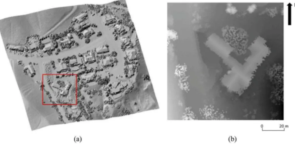
The proposed method will be explained on the Utah-5 DSM test data throughout the manuscript. This test sample (with spatial resolution of 0.5 m) is obtained from the NSF Open Topography website (http://opentopo.sdsc.edu/gridsphere/gridsphere?cid=geonli dar). Here, only thefirst pulse return is available in lidar data. The original Utah-5 test data are given inFigure 1(a). As can be seen in thisfigure, the test data contain buildings and various vegetation on a sloped terrain. More detail on it can be found inSection 4. Also, a subpart of the Utah-5 test data is picked as shown inFigure 1(b)to explain steps of the proposed method better.
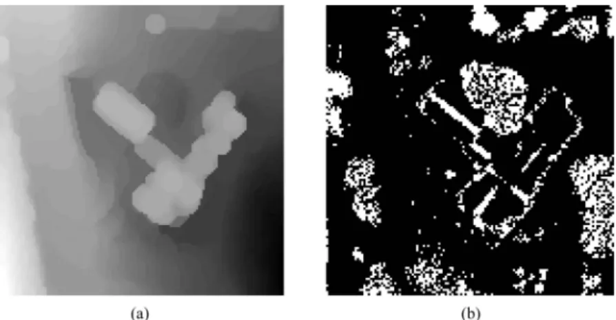
When the preprocessing step is applied on the subpart of the Utah-5 test data, the obtained result is as shown inFigure 2(a). As can be seen in thisfigure, the test data are smoothed by preprocessing. Small object detection results from this test data are also given inFigure 2(b). These will be used in the following sections.
2.2. Extracting non-ground seed points
Segmentation is applied to detect non-ground objects in DSM data in the proposed method. Thefirst step in this operation is extracting seed points. We utilized DSM data to detect buildings with a probabilistic voting method (Özcan, Ünsalan, and Reinartz
2013) in a previous study. We extend this method further to detect seed points from DMS data in this study. Let’s explain this method in detail.
Figure 1.The original Utah-5 DSM test data and its subpart to be used throughout the manuscript. The spatial resolution of DSM is 0.5 m. (a) DSM data. (b) Subpart of DSM, represented by a red box in part (a).
An object can be represented by its edges in DSM data. Therefore, Canny edge detection is applied to the DSM (Canny 1986). To note here, there are also other edge detectors in the literature. However, the Canny edge detector has better edge detection performance in remote-sensing images. Therefore, we used it in this study.
Edge detection result for the preprocessed subpart of the Utah-5 test data is as shown in Figure 3(a). As can be seen in this figure, object edge points are extracted. However, there are also some extra edges extracted because of elevation changes in the sloped terrain.
Edges are strong indicators of existence of a non-ground object. Therefore, each edge point will vote for a possible non-ground object centre location. This is done as follows. Objects are assumed to be higher than their surrounding. Therefore, an edge point, ðxe;yeÞ, is assumed to be at the centre of a wwwindow in DSM, Is. The rationale for selecting the window size will be explained in detail in Section 4.2. Each edge point votes for the highest elevation point in the window. To have a valid vote, the maximum and minimum elevation difference in the window should be greater than the elevation Figure 2.Demonstration of the preprocessing and small object detection steps on the subpart of the Utah-5 test data. (a) Preprocessing result. (b) Small object detection results by settingth=1 m.
Figure 3.Demonstration of the probabilistic object location detection method on the subpart of the Utah-5 test data. Edges and modes of the estimated pdf are given in 2D image; estimated pdf is given in 3D for better visualization. (a) Edges. (b) Estimated pdf. (c) Modes of the estimated pdf.
thresholdthused in Equation (1). The voting operation can be mathematically described as follows.
ðxm;ymÞ ¼ argmaxðx;yÞIsðx;yÞ (2) whereðxm;ymÞis the highest elevation point. Here
xe w=2 x xe þ w=2
ye w=2 y ye þ w=2
(3) The highest elevation point in the window indicates only one location for possible non-ground object centre. This may not be the exact object centre location. Therefore, an uncertainty factor is introduced by a Gaussian kernel. Hence, we cast a vote atðxm;ymÞ which leads to a Gaussian probability density function (pdf) as
pðx;yÞ ¼ ffiffiffiffiffiffi1 2π p σexp ðx xmÞ2 þ ðy ymÞ2 2σ2 ! (4) whereσis the width of the kernel. In this study,σandware kept constant. Hence, they do not change for each edge point.
Naturally, there are several edge points extracted from DSM data. Using the same procedure for each edge point, the estimated pdf for the object centre location becomes pvðx;yÞ ¼ 1 C Xi¼1 N 1 ffiffiffiffiffiffi 2π p σexp ðx xmðiÞÞ2 þ ðy ymðiÞÞ2 2σ2 ! (5) whereC is the normalizing constant,Nis the number of votes, andðxmðiÞ;ymðiÞÞis the
ith vote centre. To note here,N will be less than or equal to the total number of edge points since the elevation threshold constraint should be satisfied for an edge point to vote.
The generated pdf for the Utah-5 test data is given inFigure 3(b). As can be seen in thisfigure,pvðx;yÞis multimodal. Modes (location of local maxima) ofpvðx;yÞwill give possible non-ground object location information. Modes of the Utah-5 test data are as shown in Figure 3(c) in which each mode is represented by a triangle marker. Even though there is only one non-ground object (building) inFigure 3(c), there are multiple modes on it. This is because of the structure of the building. There are also modes in the sloped parts of the terrain which do not correspond to an object. All extracted modes will be used as seed points in the segmentation step to be explained next.
3. Segmentation of non-ground objects
The segmentation relies on two steps: a morphological-based segmentation followed by a region growing algorithm. Let’s start with explaining the initial segmentation step.
3.1. Initial segmentation
Thefirst step in DSM segmentation is based on the modes ofpvðx;yÞ. These will be used in extracting reference elevation values. Let’s assume thatMmodes are extracted. They
can be represented asðxpðjÞ;ypðjÞÞforj¼1; ;M. An initial segment can be obtained with connected pixels to eachðxpðjÞ;ypðjÞÞin an iterative manner as
Xk ¼ ðXk1BÞ \S (6) where S¼X j¼1 M IsðxpðjÞ;ypðjÞÞ Isðx;yÞ <th (7)
where ‘S’ and ‘X’ are both sets, X0 ¼SðxpðjÞ;ypðjÞÞ is the initial value, krepresents the iteration number, denotes the morphological dilation operation, and B is the 33 structuring element. If Xk¼Xk1, then the iteration stops.
Initial segmentation result on the subpart of Utah-5 test data is as shown inFigure 4.Two cases are provided here. In thefirst case, the mode is on a building. The initial segmentation result for this case is given inFigure 4(a)as white dots. As can be seen here, the initial segment partly overlaps the building. In the second case, the mode is on a terrain with slope. The initial segmentation result for this case is given inFigure 4(b)as white dots. As can be seen here, the initial segment spreads on the ground with the same elevation value.
4. Morphological region growing
The initial segmentation result is used in morphological region growing to extract possible non-ground objects. The proposed method is algorithmically explained in Listing 1. This method can be summarized as follows. The outer boundary of the initial segment is added to the segmentation result at each iteration. This is done by checking the elevation value of each pixel in the outer boundary. To append a pixel to the segment, its height should be within the given upper and lower tolerance values. Pixels satisfying the tolerance constraint are appended to the growing segment. This operation is done iteratively. The iteration ends when there is no pixel to append or the maximum iteration number is reached. Hence, the possible instability issue is avoided. The underlying assumption here is that the segment to be extracted Figure 4.Initial segmentation results on non-ground and ground. White dots indicate the initial segmentation results. (a) Non-ground segment. (b) Ground segment.
should have aflat or nearlyflat shape and it should be aboveground. Thefinal segmentation result is obtained if the mean elevation height of the grown segment is greater than the mean elevation height of the segments border pixels. Hence, a segment which is grown in aflat region is rejected. This method is performed for all modes of the voting map. Finally, all segmentation results are merged.
Algorithm 1Morphological region growing
BEGIN
ðxi;yiÞ 2Xk; points in the initial segmentation
μX¼1 N
PN
i¼1
Isðxi;yiÞ; calculate the mean elevation value
tl,tu, andts; lower, upper, andfinal elevation threshold values
Tmax; maximum iteration number
B; 33 structuring element for thickening ⊛; hit or miss transform
⊝; erosion operation
counter¼0; initialize the counter repeat
Xþk ¼Xk[ ðXk BÞ; thicken the current segment
Xþb ¼Xþk ðXþk BÞ; extract the boundary of the thickened segment Δμþ
k ¼μXIsðxb;ybÞwhere ðxb;ybÞ 2Xþb; calculate the elevation difference for each boundary pixel
if Δμþk >tu; if any boundary pixel’s elevation value is too low then Xþkðxb;ybÞ ¼0; set the related pixel to zero
end if
if Δμþk <tl!; if any boundary pixel’s elevation value is too highthen Xþkðxb;ybÞ ¼0; set the related pixel to zero
end if
if Xþk ¼Xkor counter> Tmaxthen EXIT = true; stop growing else
EXIT = false; keep growing
Xk¼Xþk; update the initial segment
μX¼1 N
PN
i¼1
Isðxi;yiÞ; update the mean elevation value counter+ = 1; increase the counter
end if untilEXIT μb¼1 M PM i¼1
Isðxbi;ybiÞ, whereðxb;ybÞ 2Xþb; calculate outer perimeter mean elevation height Δμ¼μXμb; calculate elevation height difference of the object and its outer perimeter
ifΔμ<ts; if not satisfying being an objectthen Xkðxi;yiÞ ¼0; delete all pixels
end if return Xk END
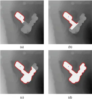
The iteration steps of the proposed morphological region growing algorithm on the initial non-ground segment (inFigure 4(a)) are as shown inFigure 5.In thisfigure, white dots indicate the segmentation result at each iteration. Red dots indicate pixels whose height is lower or higher than the upper and lower threshold values, respectively. As the region grows at each iteration, the mean height of the segment is updated. Hence, if the non-ground object is a building and has sloped orflat rooftop, the algorithm can handle it. As iterations end, the algorithm checks whether the segmentation result belongs to a non-ground object or not. For the case inFigure 5, the result belongs to a non-ground object. Therefore, thefinal segment is accepted. Iteration steps of the proposed region growing algorithm on the initial ground segment (in Figure 4(b)) are as shown in
Figure 6.For this case, thefinal segment is rejected.
4.1. Final non-ground object segmentation
The algorithm in Listing 1 is applied on all modes ofpvðx;yÞto segment all non-ground objects in DSM data. Then, they are merged with the initial small non-ground object detection result by a logical OR operation (Mano and Ciletti 2007). This step can be formulated as
Figure 5.Running form of the morphological region growing algorithm on the initial building segment. White dots indicate the segmentation result. Red dots are pixels whose height is lower or upper than the upper and lower threshold values, respectively. (a) Iteration 1. (b) Iteration 4. (c) Iteration 7. (d) Iteration 10.
O¼Os[
Xj¼1
M
XkðjÞ; (8)
where O is thefinal non-ground object segmentation result, Osis the small non-ground object detection result obtained in the preprocessing step, and XkðjÞis the segmentation result for thejth mode ofpvðx;yÞ.
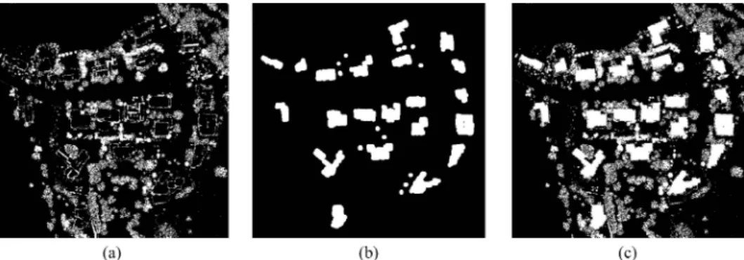
Non-ground object segmentation result for the Utah-5 test data is given inFigure 7.
Here, small object detection result is given in Figure 7(a). Segmentation via morpholo-gical region growing is given inFigure 7(b). Their combination is given inFigure 7(c). As can be seen in this figure, most non-ground objects are segmented in this test data. Quantitative results for the Utah-5 test data will be given inSection 4.
4.2. DTM generation
Non-ground pixels are extracted by segmentation in the previous section. The remaining points are taken as ground points. Hence, DTM can be generated from these. Here, we use image inpainting to generate DTM as suggested by Pingel, Clarke, and McBride (2013) and as in Özcan and Ünsalan (2017). In image inpainting, missing pixels of the image are interpolated with existing neighbour pixels (Bertalmio et al.2000). Similarly, Figure 6.Running form of the morphological region growing method on a ground segment. White dots indicate the segmentation result. Red dots are pixels whose height is lower or upper than the upper and lower threshold values, respectively. (a) Iteration 1. (b) Iteration 4. (c) Iteration 7. (d) Iteration 10.
we label the non-ground pixels in the DSM as missing andfill them with Derrico’s image inpainting method to obtain the DTM. The MATLAB code of the used method can be found athttp://www.mathworks.com/matlabcentral/fileexchange/4551-inpaint-nans. To note here, other methods can also be used here such as kriging or natural neighbours. The true DTM and generated DTM for Utah-5 are given inFigure 8.As can be seen in this figure, the generated and true DTMs are similar.
5. Experiments
We evaluate the performance of the proposed method in this section. To do so, we tested it on three different data sets. Thefirst data set is obtained from the publicly available NSF Open Topography website which provides LiDAR-based DSM. Challenging regions (to observe the limits of the proposed method) are selected from the web site and the test set is formed accordingly. The second data set is obtained from ISPRS which is used as a benchmark (Sithole and Vosselman2004). The third data set is composed of DSM generated from stereo WorldView image pairs. Industrial and residential regions are selected here.
th¼
Non-ground object segmentation results for the Utah-5 DSM test data. Threshold is selected as th¼1.
Next, we will summarize the performance evaluation criteria used in reporting experi-mental results. Then, we will focus on parameter settings and sensitivity analysis. Finally, we will provide the experimental results on three different data sets.
5.1. Performance evaluation criteria
The performance of the proposed method is provided in terms of non-ground object detection results for all data sets. In this study, several evaluation metrics are used. Specifically,κ, total error (TE), type-I error (TI), and type-II error (TII) are used for thefirst and third data sets (Cohen1968; Sithole and Vosselman2004). Type I error is equal to the number of ground pixels mistakenly classified as non-ground divided by the true number of ground pixels. Type II error is equal to the number of non-ground pixels mistakenly classified as ground divided by the true number of non-ground pixels. Total error is the number of all false classifications divided by the total number of pixels. Finally,κis the statistical measure that is more robust than simple per cent agreement. It is calculated using proportional agreement between ground and non-ground pixels and the expected agreement by chance. While performing error calculations, all pixels are taken into account. Hence, none of the pixels are left behind.
Completeness (CP), correctness (CR), andF1 score metrics are also used in thefirst and second data sets. Hence, the results can be compared with other methods using the first data set (Rutzinger, Rottensteiner, and Pfeifer 2009). These metrics are defined as follows. CP ¼ ðTPÞ ðTPÞ þ ðFNÞ (9) CR ¼ ðTPÞ ðTPÞ þ ðFPÞ (10) F1 ¼ 2ðTPÞ 2ðTPÞ þ ðFPÞ þ ðFNÞ (11)
where true-positive (TP), false-positive (FP), and false-negative (FN) values are used in calculations.
5.2. Parameter settings and sensitivity analysis
Through the voting and segmentation steps, it is assumed that a non-ground object is at least 1 m above the ground. Therefore, the elevation threshold in Equation (1) is selected as th¼1 m. This value may be increased or decreased with respect to the height of small objects to be detected. When a non-ground object is larger compared to the window size in Equation (3), votes may not accumulate at one location on the object, but may result in more than one accumulation point. This may cause multiple peaks in the estimated pdf. On the other hand, if the window size is selected too large, then some objects may not be detected. As a compromise, the voting window size in Equation (3) is selected as w¼3 m. To note here, the minimum size of objects also depends on the DSM resolution. The width of the Gaussian kernel in Equation (5) also
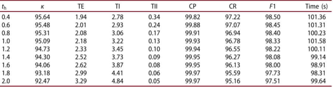
in the algorithm and changed the thresholdthfrom 0.4 to 2.0 m. We provide the obtained results inTable 1. Here, we provide all performance criteria with respect toth. We also provide the total time (in seconds) needed to process all test data at hand. As can be seen in this table, performance of the proposed method is fairly insensitive to the changes inth. Besides, the total computation time does not change significantly with respect to change inth.
We nextfixed all the parameters and only changed the window sizewfrom 3 to 19 m. We provided the obtained results inTable 2. As can be seen in this table, performance of the proposed method is also fairly insensitive to a change in window sizew. However, the total computation time decreases with respect to increasing window size.
5.3. NSF Open Topography lidar data set
Thefirst data set is obtained from the publicly available NSF Open Topography website. The reader can download the lidar point cloud data by defining an area of interest from Table 1.Sensitivity analysis of the proposed method with respect to change inth value.
th κ TE TI TII CP CR F1 Time (s) 0.4 95.64 1.94 2.78 0.34 99.82 97.22 98.50 101.36 0.6 95.48 2.01 2.93 0.24 99.88 97.07 98.45 101.31 0.8 95.31 2.08 3.06 0.17 99.91 96.94 98.40 100.23 1.0 95.09 2.18 3.22 0.13 99.93 96.78 98.33 101.58 1.2 94.73 2.33 3.45 0.10 99.94 96.55 98.22 100.11 1.4 94.30 2.52 3.73 0.09 99.95 96.27 98.08 99.14 1.6 94.06 2.62 3.87 0.08 99.95 96.13 98.00 98.91 1.8 93.18 2.99 4.41 0.06 99.97 95.59 97.73 98.31 2.0 92.47 3.29 4.84 0.05 99.97 95.16 97.51 99.64
Table 2.Sensitivity analysis of the proposed method with respect to change inw value.
w κ TE TI TII CP CR F1 Time (s) 3 93.81 2.72 4.02 0.10 99.95 95.98 97.92 104.67 5 95.09 2.18 3.22 0.13 99.93 96.78 98.33 101.58 7 95.48 2.01 2.97 0.18 99.91 97.03 98.45 95.56 9 95.31 2.10 2.84 0.78 99.64 97.16 98.38 95.63 11 95.34 2.07 2.68 1.07 99.51 97.32 98.40 91.95 13 95.38 2.03 2.49 1.36 99.40 97.51 98.45 92.08 15 95.59 1.93 2.26 1.62 99.32 97.74 98.52 91.11 17 95.26 2.07 2.15 2.31 98.99 97.85 98.42 88.80 19 95.30 2.04 1.87 2.80 98.76 98.13 98.44 89.61
this website. The reader can also download DTM of the selected area from the men-tioned website. The point density for the NSF Open Topography lidar data set is 9.14 points/m2. More information on this data set can be found inhttp://opentopo.sdsc.edu/ datasetMetadata?otCollectionID=OT.072017.26912.1.
Nine test samples are picked from the NSF Open Topography website. These are labelled Utah 1–9 throughout the study. The selected subarea shows residential char-acteristics with buildings. DSM data for all test samples are given inFigure 9.The grid resolution for all test samples is 0.5 m. The DTM for this data set is also available on the website. Due to the lack of manually generated ground truth for test samples, the downloaded DTM is used to form the ground truth. Therefore, provided results in this section will be relative to the downloaded DTM.
Test samples in thefirst data set are grouped into three parts according to the terrain type, object size, and type as follows. Test samples Utah 1–3 haveflat terrain; buildings here are mostly in one piece. Building layout in these test samples changes from small to large. There are trees on the side of roads and buildings. On these samples, the proposed method is tested for segmenting objects with varying size located on a flat terrain. In Utah-1, there is one large building with an irregular shape. In Utah-2, there is one large building withflat roof. In Utah-3, buildings mostly have equal size with four of them having different size. Utah 4–6 test data have sloped terrain with regular-sized separate buildings. In Utah-4, buildings are surrounded by trees. In Utah-5 and Utah-6, Figure 9.DSM data for thefirst data set. First row: Utah 1–3; second row: Utah 4–6; third row: Utah 7–9.
are used as suggested in Pingel, Clarke, and McBride (2013). The second method is proposed by Mongus, Lukac, and Zalik (2014). This method is also based on morpholo-gical operations. It uses a top-hat scale-space transform using differential morphological profiles on point’s residuals from the approximated surface. Surface and regional fea-tures are used for building detection. The software for this method is called gLiDAR and can be obtained fromhttp://gemma.uni-mb.si/gLiDAR/about.html. Within this software, default parameter values are used as suggested in Mongus, Lukac, and Zalik (2014). The third groundfiltering method is based on EMD (Özcan and Ünsalan2017). This method applies two-dimensional EMD with morphological modifications in an adaptive manner forfiltering non-ground object pixels.
For the assessment of these methods, ground-truth object locations are formed as follows. First, the ground-truth DTM is subtracted from DSM and the normalized DSM is obtained. Then, pixels above 1 m (in the normalized DSM) are considered as belonging to a non-ground object. Remaining pixels are taken as ground. Since SMRF, gLiDAR, and EMD filtering methods generate DTM, the same procedure is applied to segment non-ground objects.
Generated and true DTMs for Utah 1-2-7-8-9 are given in Figure 10, respectively. As can be seen in this figure, all other three methods in the literature had problems in filtering large buildings. Detailed non-ground object segmentation results are given in
Figure 11.The problem in detecting large buildings is clearly seen in thisfigure. All three methods in the literature have misdetections on large objects. However, the proposed method only has a misdetection problem on objects which are connected to nearby higher objects. This is because of the segmentation algorithm. At the end of segmenta-tion, it is assumed that the object is taller than its immediate neighbours. Hence, it is tested whether the elevation height difference of the segmented object and its peri-meter is above a threshold. This assumption may fail when buildings are connected side by side and one is taller than the other. Part of the largest building is lower than its surrounding for all directions in the Utah-1 test data. Hence, it could not be detected. The reason for this result can be explained as follows. The missing part did not get sufficient votes at the probabilistic voting step. Hence, no segmentation has started there. The SMRF and EMD methods also had a problem in detecting the same part of the building. gLiDAR did not detect most parts of the same building. There are also similar results on the Utah 7-8-9 test samples. Here, some buildings which are connected to a taller building could not be detected by the proposed method.
The object segmentation performance of the proposed and other three methods is tabulated in Table 3. As can be seen in this table, the proposed method performs slightly worse than SMRF and EMD and better than gLiDAR in terms of all metrics on the Utah-1 test data. The proposed method performs better than the other three methods on the Utah-2 test data. Here, the other three methods have large TI error because of the misdetection of the largest building. All three methods have similar results on the Utah-3 test data. For the Utah 4–6 test data, obtained result by the proposed method is similar to other methods even though the terrain is sloped and the proposed method is not based on generated DTM. The proposed method has misdetections on the Utah-7 test data. Therefore, it has a high TI error. The proposed method has the best K, TE, TI, and TII values on the Utah 8–9 test data. These results can be summarized as follows. If buildings are not large in the test data (as in Utah-3), all four methods have good results. If there are large buildings in the test data (as in Utah-1-2-7-8-9), other methods mostly fail where the proposed method works prop-erly. On a sloped terrain, SMRF has the best score with the proposed and gLiDAR methods having similar values. The proposed method outperforms other methods on segmenting connected and large buildings.
Results inTable 3can be summarized as follows. The proposed method has the best meanκ with 95.09% where SMRF, gLiDAR, and EMD meanκ are 89.36%, 89.48%, and 87.10%, respectively. The proposed method has the best mean TE, TI, and TII values with 2.18%, 3.22%, and 0.13%, respectively. It also has the lowest standard deviation of all metrics. This shows the robustness of the proposed method on such a diverse test set. Figure 10.Generated DTM results for the Utah-1, Utah-2, Utah-7, Utah-8, and Utah-9 test data. The first column corresponds to DSM data. The second to last columns correspond to true DTM, proposed method, SMRF, gLiDAR, and EMD-filtering results, respectively.
The CP, CR, and F1 scores are also provided for the first data set in Table 4. Here, pixel-wise building detection results are given. The mean CP and CR scores are 99.93% and 96.78%, respectively. The meanF1 score, which is harmonic mean of completeness and correctness, is 98.33%. These results indicate that the proposed method works fairly well on thefirst data set.
5.4. ISPRS Vaihingen data set
The second data set (provided by ISPRS) consists of semantically labelled lidar data for Vaihingen, Germany. The point density for the ISPRS Vaihingen data set is 4 points/m2. The subarea shows residential and urban characteristics with dense buildings. More information on this data set can be found in http://www2.isprs.org/commissions/ comm3/wg4/detection-and-reconstruction.html#VaihigenDataDescr.
Figure 11.Detailed object segmentation results for the Utah 1-2-7-8-9 test data. Columns from left to right correspond to the proposed method, SMRF, gLiDAR, and EMD-filtering results, respectively. True non-ground object segments are labelled in green, true ground detections are labelled in grey, undetected non-ground segments are labelled in blue, and false non-ground segments are labelled in red in thesefigures.
Table 3. Object segmentation performance of the proposed and other three methods in percentages on the NSF Open Topography lidar data set. Proposed method SMRF gLiDAR EMD Test κ TE TI TII κ TE TI TII κ TE TI TII κ TE TI TII Utah-1 97.34 1.08 1.48 0.02 97.86 0.87 1.19 0.03 91.87 3.22 4.32 0.03 97.83 0.88 1.21 0.05 Utah-2 98.59 0.65 1.01 0.03 83.27 7.45 10.52 0.07 83.39 7.40 10.44 0.14 83.06 7.55 10.61 0.18 Utah-3 97.53 1.14 1.76 0.03 99.36 0.30 0.45 0.03 98.83 0.54 0.82 0.05 99.48 0.24 0.34 0.07 Utah-4 97.12 1.43 2.41 0.28 97.97 1.01 1.60 0.32 97.09 1.45 2.55 0.13 97.89 1.05 1.04 1.06 Utah-5 97.28 0.96 1.14 0.31 98.35 0.58 0.66 0.30 96.78 1.13 1.40 0.18 98.02 0.70 0.53 1.28 Utah-6 94.57 2.43 3.45 0.33 96.59 1.54 2.01 0.60 94.18 2.60 3.70 0.32 97.06 1.33 1.48 1.06 Utah-7 87.40 6.08 9.65 0.09 83.49 7.94 12.14 0.33 87.49 6.05 9.52 0.24 77.38 10.81 15.58 1.26 Utah-8 97.21 0.97 1.24 0.02 74.09 8.07 9.48 0.06 82.79 5.60 6.71 0.39 69.24 9.50 10.53 3.42 Utah-9 88.78 4.85 6.81 0.07 73.21 11.07 14.24 0.46 72.87 11.21 14.31 0.88 63.93 14.57 17.72 2.10 Mean 95.09 2.18 3.22 0.13 89.36 4.31 5.81 0.25 89.48 4.36 5.98 0.26 87.10 5.18 6.56 1.16 Min 87.40 0.65 1.01 0.02 73.21 0.30 0.45 0.03 72.87 0.54 0.82 0.03 63.93 0.24 0.34 0.05 Max 98.59 6.08 9.65 0.33 99.36 11.07 14.24 0.60 98.83 11.21 14.31 0.88 99.48 14.57 17.72 3.42 Standard deviation 4.12 1.96 3.03 0.13 10.87 4.23 5.65 0.21 8.57 3.51 4.61 0.26 14.01 5.46 7.06 1.09
Trees and vegetation are removed by using an NDVI mask from object detection results in the second data set. Therefore, it is assumed that the remaining object segmentation results represent buildings. Hence, the performance of the proposed method was evaluated on building detection results of the ISPRS reference data. To be compatible with other methods in the literature using this data set, the CP, CR, and
F1 score results are given in Table 5. Here, pixel-wise building detection results are provided. As can be seen in this table, mean CP and CR scores are close where mean CP is 90.33% and mean CR is 88.92%. The meanF1 score is 89.57%. The reader can check the most recent comparison results from the mentioned ISPRS website (http://www2. isprs.org/commissions/comm3/wg4/2d-sem-label-vaihingen.html). To note here, most of the other methods use supervised approaches on the ISPRS data. Although the pro-posed method has an unsupervised approach, it still provides good results.
Building detection results on three test samples from the second data set are given in
Figure 12.As can be seen in thisfigure, most buildings are detected. In cases where a building is partly surrounded by taller buildings or trees, some misdetections occur. Such a case can be seen in the last row ofFigure 12, where a building is surrounded by trees at the bottom centre of the test data. Hence, it could not be detected.
5.5. Worldview stereo image-based DSM data set
The third data set is composed of DSM generated from WorldView-2 stereo image pairs. The WorldView-2 image pair has been acquired over Istanbul, Turkey, on 7 July 2012. The convergence (stereo) angle is 15º, which equals a base to height ratio of approxi-mately 2:1. The pixel resolution is 0.5 m, allowing to derive a quite dense regular point cloud of disparities. The WorldView-2 DSM (pixel spacing 0.5 m) has been generated using a robust dense stereo matching algorithm based on semi-global matching using a
Vaihingen data set.
Test CP CR F1 Vaihingen-1 93.63 85.78 89.53 Vaihingen-2 88.30 89.40 88.80 Vaihingen-3 89.41 87.72 88.55 Vaihingen-4 89.10 91.00 90.00 Vaihingen-5 91.22 90.69 90.95
combination of census and mutual information as cost functions developed by the institution of one of the authors (dAngelo and Reinartz2011; Arefiand Reinartz 2013). Interpolation has been performed using the delta surfacefill methodology, preserving also height jumps (dAngelo and Reinartz2012).
In the third test set, sharpness of the DSM is slightly worse compared to thefirst data set. This affects building boundaries such that they have smoother transitions towards the ground. Therefore, this data set shows how the proposed method works under these constraints.
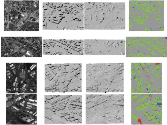
In thefirst column ofFigure 13, four panchromatic test images where thefirst two are residential and the last two are industrial regions in Istanbul, Turkey are provided. In the second column of the same figure, DSM data of the same locations are provided. In residential regions, buildings have regular size, but closely located buildings look like Figure 12.Building detection results on the Vaihingen 1-3-5 of ISPRS data set. Columns from left to right correspond to the 2D image, DSM, and building detection results, respectively. In the last column, true non-ground object segments are labelled in green, true ground detections are labelled in grey, undetected non-ground segments are labelled in blue, and false non-ground segments are labelled in red.
connected due to the nature of the DSM data. In industrial regions, some buildings have very large footprints. In the third column, generated DTMs are given. In the last column, object detection results are given. Due to the lack of ground-truth information for object locations, they are extracted manually.
Quantitative results of the WorldView stereo image-based DSM data set are given in
Table 6. Unfortunately, the other three methods could not be used on this data set since they need lidar points as input. The proposed method performs well in residential regions where the κ for the first two data set is over 85%. In industrial regions, κ decreases. False detections cause large TII error in these test data. There are some embankments where one side of them looks like an object and the other side looks Figure 13.Filtering results on the WorldView stereo image-based DSM data set. Columns from left to right correspond to panchromatic image, DSM, generated DTM, and object filtering results, respectively. True non-ground object segments are labelled in green, true ground detections are labelled in grey, undetected non-ground segments are labelled in blue, and false non-ground segments are labelled in red in thesefigures.
Table 6.Object segmentation performance of the proposed method in percen-tages on the WorldView stereo image-based DSM data set.
Test κ TE TI TII Residential-1 86.71 4.64 5.26 2.24 Residential-2 86.28 5.27 6.44 1.49 Industrial-1 83.44 6.45 6.12 7.40 Industrial-2 79.25 9.18 7.71 12.24 Mean 83.92 6.39 6.38 5.84
like belonging to the terrain in the Industrial-1 test data. Thus, it misguides the seg-mentation process and causes false detection (in red at the upper right corner of the image). There is a bridge in the Industrial-2 test data which is correctly segmented as an object. However, the terrain which is connected to the bridge was also segmented as an object, which caused a large TII error. In the upper right of the same test data, part of a large building could not be segmented. Even though the building has aflat roof, it has an irregular distribution of height data on its roof. Hence, the segmentation method did not work properly.
6. Conclusions
In this study, a novel ground filtering and DTM generation method is proposed. The key idea of the method is based on the assumption that non-ground objects are higher than their surrounding. The method consists of probabilistic voting and novel morphological region growing-based segmentation steps. Obtained segments are used for DTM generation. We tested the proposed method on two different lidar and one stereo image-based DSM data sets. Experimental results indicate that the proposed method works fairly well on both flat and sloped terrain. Furthermore, it performs better infiltering large buildings compared to other methods in the litera-ture. Besides, the proposed method is insensitive to object size to be filtered. This is the most advantageous point of the proposed method compared to those available in the literature. The proposed method has some misdetections due to the structure of complex buildings. This will be the focus of future work. There is also one possible extension for the proposed method in this study. Instead of the nearest neighbour interpolation, DSM computation can be performed by selecting the maximum eleva-tion per grid cell and further interpolating the empty cells. This may improve the performance of the proposed method.
Disclosure statement
No potential conflict of interest was reported by the authors.
Funding
This work is supported by TUBITAK through project no 114E199.
References
Arefi, H., and P. Reinartz.2013.“Building Reconstruction Using DSM and Orthorectified Images.”
Remote Sensing5: 1681–1703. doi:10.3390/rs5041681.
Axelsson, P. 2000. “DEM Generation from Laser Scanner Data Using Adaptive TIN Models.”
International Archives of Photogrammetry and Remote Sensing33 ofB4/1(PART 4): 111–118.
Bertalmio, M., G. Sapiro, V. Caselles, and C. Ballester.2000.“Image Inpainting.”InProceedings of the
27th Annual Conference on Computer Graphics and Interactive Techniques, Louisiana, USA, July
23-28. 417–424.
Canny, J. 1986. “A Computational Approach to Edge Detection.” IEEE Transactions on Pattern
Hu, H., Y. Ding, Q. Zhu, B. Wu, H. Lin, Z. Du, Y. Zhang, and Y. Zhang.2014.“An Adaptive Surface Filter for Airborne Laser Scanning Point Clouds by Means of Regularization and Bending Energy.” ISPRS Journal of Photogrammetry and Remote Sensing 92: 98–111. doi:10.1016/j. isprsjprs.2014.02.014.
Hui, Z., Y. Hu, Y. Z. Yevenyo, and X. Yu.2016.“An Improved Morphological Algorithm for Filtering Airborne LiDAR Point Cloud Based on Multi-Level Kriging Interpolation.”Remote Sensing8 (1): 35. doi:10.3390/rs8010035.
Kraus, K., and N. Pfeifer.1997. “A New Method for Surface Reconstruction from Laser Scanner Data.”International Archives of Photogrammetry and Remote Sensing32: 80–86.
Kraus, K., and N. Pfeifer.1998.“Determination of Terrain Models in Wooded Areas with Airborne Laser Scanner Data.” ISPRS Journal of Photogrammetry and Remote Sensing 53: 193–203. doi:10.1016/S0924-2716(98)00009-4.
Kraus, K., and N. Pfeifer.2001.“Advanced DTM Generation from LiDAR Data.”International Archives
Of Photogrammetry Remote Sensing And Spatial Information Sciences34 (3): 23–30.
Li, Y.2013.“Filtering Airborne LiDAR Data by an Improved Morphological Method Based on Multi-Gradient Analysis.” ISPRS–International Archives of the Photogrammetry, Remote Sensing and
Spatial Information Sciences40: 191–194. doi:10.5194/isprsarchives-XL-1-W1-191-2013.
Mano, M. M., and M. D. Ciletti.2007.Digital Design. 4th ed. New Jersey, NJ: Pearson.
Meng, X., N. Currit, and K. Zhao.2010.“Ground Filtering Algorithms for Airborne LiDAR Data: A Review of Critical Issues.”Remote Sensing2: 833–860. doi:10.3390/rs2030833.
Mongus, D., N. Lukac, and B. Zalik.2014.“Ground and Building Extraction from LiDAR Data Based on Differential Morphological Profiles and Locally Fitted Surfaces.” ISPRS Journal of
Photogrammetry and Remote Sensing93: 145–156. doi:10.1016/j.isprsjprs.2013.12.002.
Mongus, D., and B. Zalik.2012.“Parameter-Free Ground Filtering of LiDAR Data for Automatic DTM Generation.” ISPRS Journal of Photogrammetry and Remote Sensing 67: 1–12. doi:10.1016/j. isprsjprs.2011.10.002.
Mongus, D., and B. Zalik.2014.“Computationally Efficient Method for the Generation of a Digital Terrain Model from Airborne LiDAR Data Using Connected Operators.”IEEE Journal of Selected
Topics in Applied Earth Observations and Remote Sensing 7 (1): 340–351. doi:10.1109/
JSTARS.2013.2262996.
Özcan, A. H., and C. Ünsalan.2017.“LiDAR Data Filtering and DTM Generation Using Empirical Mode Decomposition.”IEEE Journal of Selected Topics in Applied Earth Observations and Remote
Sensing10 (1): 360–371. doi:10.1109/JSTARS.2016.2543464.
Özcan, A. H., C. Ünsalan, and P. Reinartz.2013.“Building Detection Using Local Features and DSM Data.”Proceedings of RAST’13, Istanbul, Turkey, June 12–14, 139–143.
Pingel, T. J., K. C. Clarke, and W. A. McBride.2013.“An Improved Simple Morphological Filter for the Terrain Classification of Airborne LiDAR Data.” ISPRS Journal of Photogrammetry and Remote
Rutzinger, M., F. Rottensteiner, and N. Pfeifer.2009.“A Comparison of Evaluation Techniques for Building Extraction from Airborne Laser Scanning.” IEEE Journal of Selected Topics in Applied
Earth Observations and Remote Sensing2 (1): 11–20. doi:10.1109/JSTARS.2009.2012488.
Shan, J., and S. Aparajithan. 2005. “Urban DEM Generation from Raw Lidar Data: A Labeling Algorithm and Its Performance.” Photogrammetric Engineering and Remote Sensing 71 (2): 217–226. doi:10.14358/PERS.71.2.217.
Sithole, G. 2001. “Filtering of Laser Altimetry Data Using a Slope Adaptive Filter.” International
Archives of Photogrammetry Remote Sensing and Spatial Information Sciences34: 203–210.
Sithole, G., and G. Vosselman.2004.“Experimental Comparison of Filter Algorithms for bare-Earth Extraction from Airborne Laser Scanning Point Clouds.”ISPRS Journal of Photogrammetry and
Remote Sensing59: 85–101. doi:10.1016/j.isprsjprs.2004.05.004.
Susaki, J.2012.“Adaptive Slope Filtering of Airborne Lidar Data in Urban Areas for Digital Terrain Model (Dtm) Generation.”Remote Sensing4 (6): 1804–1819. doi:10.3390/rs4061804.
Vega, C., S. Durrieu, J. Morel, and T. Allouis. 2012. “A Sequential Iterative Dual-Filter for Lidar Terrain Modeling Optimized for Complex Forested Environments.”Computers and Geosciences
44: 3141. doi:10.1016/j.cageo.2012.03.021.
Vosselman, G. 2000. “Slope Based Filtering of Laser Altimetry Data.” International Archives of
Photogrammetry and Remote Sensing33: 935–942.
Wang, C. K., and Y. H. Tseng.2010.“DEM Generation from Airborne LiDAR Data by an Adaptive Dual-Directional Slope Filter.”ISPRS TC VII SymposiumXXXVIII (Part 7B): 628–632.
Zhang, J., and X. Lin.2013.“Filtering Airborne LiDAR Data by Embedding Smoothness-Constrained Segmentation in Progressive TIN Densification.”ISPRS Journal of Photogrammetry and Remote
Sensing81: 44–59. doi:10.1016/j.isprsjprs.2013.04.001.
Zhang, K., S. C. Chen, D. Whitman, M. L. Shyu, J. Yan, and C. Zhang. 2003. “A Progressive Morphological Filter for Removing Nonground Measurements from Airborne LiDAR Data.”IEEE