Lukas Kremens and Ian Martin
The quanto theory of exchange rates
Article (Accepted version)
(Refereed)
Original citation:
Kremens, Lukas and Martin, Ian (2018) The quanto theory of exchange rates. American Economic Review. ISSN 0002-8282 (In Press)
© 2018 American Economic Association
This version available at: http://eprints.lse.ac.uk/89839/ Available in LSE Research Online: August 2018
LSE has developed LSE Research Online so that users may access research output of the School. Copyright © and Moral Rights for the papers on this site are retained by the individual authors and/or other copyright owners. Users may download and/or print one copy of any article(s) in LSE Research Online to facilitate their private study or for non-commercial research. You may not engage in further distribution of the material or use it for any profit-making activities or any commercial gain. You may freely distribute the URL (http://eprints.lse.ac.uk) of the LSE Research Online website.
This document is the author’s final accepted version of the journal article. There may be differences between this version and the published version. You are advised to consult the publisher’s version if you wish to cite from it.
The Quanto Theory of Exchange Rates
Lukas Kremens
Ian Martin
∗August, 2018
Abstract
We present a new identity that relates expected exchange rate appreciation to a risk-neutral covariance term, and use it to motivate a currency forecasting variable based on the prices of quanto index contracts. We show via panel re-gressions that the quanto forecast variable is an economically and statistically significant predictor of currency appreciation and of excess returns on currency trades. Out of sample, the quanto variable outperforms predictions based on uncovered interest parity, on purchasing power parity, and on a random walk as a forecaster of differential (dollar-neutral) currency appreciation.
JEL codes: G12, G15, F31, F37, F47.
∗Kremens: l.kremens@lse.ac.uk, LSE. Martin: i.w.martin@lse.ac.uk, LSE. We thank the Systemic
Risk Centre and the Paul Woolley Centre at the LSE for their support, and for providing access to data sourced from Markit under license. We are grateful to Christian Wagner, Tarek Hassan, John Campbell, Mike Chernov, Gino Cenedese, Anthony Neuberger, Dagfinn Rime, Urban Jermann, Bryn Thompson-Clarke, Adrien Verdelhan, Bernard Dumas, Pierpaolo Benigno, Alan Taylor, Daniel Ferreira, Ulf Axelson, Scott Robertson, and to participants in seminars at the LSE, Imperial College, Cass Business School, LUISS, BI Business School, Boston University, and Queen Mary University of London, for their comments; and to Lerby Ergun for research assistance. Ian Martin is also grateful
It is notoriously hard to forecast movements in exchange rates. A large part of the literature is organized around the principle of uncovered interest parity (UIP), which predicts that expected exchange rate movements offset interest rate differentials and therefore equalise expected returns across currencies. Unfortunately many authors, starting from Hansen and Hodrick (1980) and Fama (1984), have shown that this prediction fails: returns have historically been larger on high interest rate currencies than on low interest rate currencies.1
Given its empirical failings, it is worth reflecting on why UIP represents such an enduring benchmark in the FX literature. The UIP forecast has three appealing prop-erties. First, it is determined by asset prices alone rather than by, say, infrequently updated and imperfectly measured macroeconomic data. Second, it has no free pa-rameters: with no coefficients to be estimated in-sample or “calibrated,” it is perfectly suited to out-of-sample forecasting. Third, it has a straightforward interpretation as the expected exchange rate movement perceived by a risk-neutral investor. Put differ-ently, UIP holds if and only if the risk-neutral expected appreciation of a currency is equal to itsreal-world expected appreciation, the latter being the quantity relevant for forecasting exchange rate movements.
There is, however, no reason to expect that the real-world and risk-neutral expecta-tions should be similar. On the contrary, the modern literature in financial economics has documented that large and time-varying risk premia are pervasive across asset classes, so that risk-neutral and real-world distributions are very different from one another: in other words, the perspective of a risk-neutral investor is not useful from the point of view of forecasting. Thus, while UIP has been a useful organizing principle for the empirical literature on exchange rates, its predictive failure is no surprise.2
In this paper we propose a new predictor variable that also possesses the three appealing properties mentioned above, but which does not require that one takes the perspective of a risk-neutral investor. This alternative benchmark can be interpreted as
1Some studies (e.g. Sarno, Schneider and Wagner, 2012) find that currencies with high interest
rates appreciate on average, exacerbating the failure of UIP; this has become known as the forward premium puzzle. Others, such as Hassan and Mano (2016), find that exchange rates move in the direction predicted by UIP, though not by enough to offset interest rate differentials.
2Various authors have fleshed out this point in the context of equilibrium models: see for example
Verdelhan (2010), Hassan (2013), and Martin (2013b). On the empirical side, authors including Menkhoff et al. (2012), Barroso and Santa-Clara (2015) and Della Corte, Ramadorai and Sarno (2016) have argued that it is necessary to look beyond interest rate differentials to explain the variation in currency returns.
the expected exchange rate movement that must be perceived by a risk-averse investor with log utility whose wealth is invested in the stock market. (To streamline the discussion, this description is an oversimplification and strengthening of the condition we actually need to hold for our approach to work, which is based on a general identity presented in Result 1.) This approach has been shown by Martin (2017) and Martin and Wagner (2018) to be successful in forecasting returns on the stock market and on individual stocks, respectively.
It turns out that such an investor’s expectations about currency returns can be inferred directly from the prices of so-called quanto contracts. For our purposes, the important feature of such contracts is that their prices are sensitive to the correlation between a given currency and some other asset price. Consider, for example, a quanto contract whose payoff equals the level of the S&P 500 index at time T, denominated in euros (that is, the exchange rate is fixed—in this example, at 1 euro per dollar—at initiation of the trade). The value of this contract is sensitive to the correlation between the S&P 500 index and the dollar/euro exchange rate. If the euro appreciates against the dollar at times when the index is high, and depreciates when the index is low, then this quanto contract is more valuable than a conventional, dollar-denominated, claim on the index.3
We show that the relationship between currency-i quanto forward prices and con-ventional forward prices on the S&P 500 index reveals the risk-neutral covariance be-tween currencyiand the index. Quantos therefore signal which currencies are risky—in that they tend to depreciate in bad times, i.e., when the S&P 500 declines—and which are hedges; it is possible, of course, that a currency is risky at one point in time and a hedge at another. Intuitively, one expects that a currency that is (currently) risky should, as compensation, have higher expected appreciation than predicted by UIP, and that hedge currencies should have lower expected appreciation. Our framework formalizes this intuition. It also allows us to distinguish between variation in risk premia across currencies and variation over time.
It is worth emphasizing various assumptions that we do not make. We do not require that markets are complete (though our approach remains valid if they are). We do not assume the existence of a representative agent, nor do we assume that
3A different type of quanto contract—specifically, quanto CDS contracts—is used by Mano (2013)
all economic actors are rational: the forecast in which we are interested reflects the beliefs of a rational investor, but this investor may coexist with investors with other, potentially irrational, beliefs. And we do not assume lognormality, nor do we make any other distributional assumptions: our approach allows for skewness and jumps in exchange rates. This is an important strength of our framework, given that currencies often experience crashes or jumps (as emphasized by Brunnermeier, Nagel and Pedersen (2008), Jurek (2014), Della Corte et al. (2016), Chernov, Graveline and Zviadadze (2018) and Farhi and Gabaix (2016), among others), and are prone to structural breaks more generally. The approach could even be used, in principle, to compute expected returns for currencies that are currently pegged but that have some probability of jumping off the peg. To the extent that skewness and jumps are empirically relevant, this fact will be embedded in the asset prices we use as forecasting variables.
Our approach is therefore well adapted to the view of the world put forward by Burnside et al. (2011), who argue that the attractive properties of carry trade strategies in currency markets may reflect the possibility of peso events in which the stochastic discount factor takes extremely large values. Investor concerns about such events, if present, should be reflected in the forward-looking asset prices that we exploit, and thus our quanto predictor variable should forecast high appreciation for currencies vulnerable to peso events even if no such events turn out to happen in sample.
We derive these and other theoretical results in Section 1, and test them in Sec-tion 2 by running panel currency-forecasting regressions. The estimated coefficient on the quanto predictor variable is economically large and statistically significant: in our headline regression (20), we find t-statistics of 3.2 and 2.3 respectively with and without currency fixed effects. (Here, as throughout the paper, we compute standard errors—and more generally the entire covariance matrix of coefficient estimates—using a nonparametric block bootstrap to account for heteroskedasticity, cross-sectional cor-relation across currencies, and autocorcor-relation in errors induced by overlapping obser-vations.) The quanto predictor outperforms forecasting variables such as the interest rate differential, average forward discount, and the real exchange rate as a univariate forecaster of currency excess returns. On the other hand, we find that some of these variables—notably the real exchange rate and average forward discount—interact well with our quanto predictor variable, in the sense that they substantially raiseR2 above what the quanto variable achieves on its own. We interpret this fact, through the
lens of the identity (6) of Result 1, as showing that these variables help to measure deviations from the log investor benchmark. We also show that the quanto predic-tor variable—that is, forward-looking risk-neutral covariance—predicts future realized covariance and substantially outperforms lagged realized covariance as a forecaster of exchange rates.
An important challenge is that our dataset spans a relatively short time period. If we assess the significance of joint hypothesis tests by using p-values based on the
asymptotic distributions of test statistics (with bootstrapped covariance matrices, as always), we find, in our pooled regressions, that the estimated coefficients on the quanto predictor variable and interest rate differential are consistent with the predictions of the log investor benchmark, but we can reject the hypothesis that, in addition, the intercept is zero. This rejection can be attributed to US dollar appreciation, during our sample, that was not anticipated by our model. But using asymptotic distributions of test statistics to assessp-values risks giving a false impression of precision, in view of our short sample period. In Section 2.6, we bootstrap the small-sample distributions of the relevant test statistics to account for this issue. When we use the associated, more conservative, small-sample p-values, we do not reject even the most optimistic hypothesis in any of the specifications, though the individual significance of the quanto predictor becomes more marginal, withp-values ranging from 5.1% to 9.7%.
In Section 3 we show that the quanto variable performs well out of sample. We focus on forecasting differential returns on currencies in order to isolate the cross-sectional forecasting power of the quanto variable in a dollar-neutral way, in the spirit of Lustig, Roussanov and Verdelhan (2011), and independent of what Hassan and Mano (2016) refer to as the dollar trade anomaly. (As noted in the preceding paragraph, the dollar strengthened against almost all other currencies over our relatively short sample, so quantos are not successful in forecasting the average performance of the dollar itself. Our findings are therefore complementary to Gourinchas and Rey (2007), who use a measure of external imbalances to forecast the appreciation of the dollar against a trade- or FDI-weighted basket of currencies.)
In a recent survey of the literature, Rossi (2013) emphasizes that the exchange-rate forecasting literature has struggled to overturn the frustrating fact, originally documented by Meese and Rogoff (1983), that it is hard even to outperform a random walk forecast out of sample. Our out-of-sample forecasts exploit the fact that our theory
makes an a priori prediction for the coefficient on the quanto predictor variable. When the coefficient is fixed at the level implied by the theory, we end up with a forecast of currency appreciation that has no free parameters, and which is therefore—like the UIP and random walk forecasts—perfectly suited for out-of-sample forecasting. Following Meese and Rogoff (1983) and Goyal and Welch (2008), we compute mean squared error for the differential currency forecasts made by the quanto theory and by three competitor models: UIP, which predicts currency appreciation through the interest rate differential; PPP, which uses past inflation differentials (as a proxy for expected inflation differentials) to forecast currency appreciation; and the random walk forecast. The quanto theory outperforms all three competitors. We also show that it outperforms on an alternative performance benchmark, the correct classification frontier, that has been proposed by Jord`a and Taylor (2012).
1
Theory
We start with the fundamental equation of asset pricing,
Et
Mt+1Ret+1
= 1, (1)
since this will allow us to introduce some notation. Today is timet; we are interested in assets with payoffs at timet+ 1. We writeEtfor the (real-world) expectation operator,
conditional on all information available at time t, and Mt+1 for a stochastic discount
factor (SDF) that prices assets denominated in dollars. (We do not assume complete markets, so there may well be other SDFs that also price assets denominated in dollars. But all such SDFs must agree withMt+1 on the prices of the payoffs in which we are
interested, since they are all tradable.) In equation (1), Ret+1 is the gross return on
some arbitrary dollar-denominated asset or trading strategy. If we write R$f,t for the gross one-period dollar interest rate, then the equation implies thatEtMt+1 = 1/R$f,t,
as can be seen by settingRet+1 =R$f,t; thus (1) can be rearranged as
EtRet+1−R$f,t=−Rf,t$ covt
Mt+1,Ret+1
. (2)
Consider a simple currency trade: take a dollar, convert it to foreign currency i, invest at the (gross) currency-iriskless rate,Ri
to dollars. We writeei,t for the price in dollars at timetof a unit of currencyi, so that
the gross return on the currency trade is Rif,tei,t+1/ei,t; setting Ret+1 =Rif,tei,t+1/ei,t in
(2) and rearranging,4 we find that
Etei,t+1 ei,t = R $ f,t Ri f,t |{z} UIP forecast −Rf,t$ covt Mt+1, ei,t+1 ei,t | {z } residual . (3)
This (well known) identity can also be expressed using the risk-neutral expectation
E∗t, in terms of which the timet price of any payoff, Xt+1, received at time t+ 1 is
time t price of a claim to Xt+1 =
1
R$f,t E
∗
t Xt+1 =Et(Mt+1Xt+1). (4)
The first equality is the defining property of the risk-neutral probability distribution. The second equality (which can be thought of as a dictionary for translating between risk-neutral and SDF notation) can be used to rewrite (3) as
E∗t ei,t+1 ei,t = R $ f,t Ri f,t . (5)
From an empirical point of view, the challenging aspect of the identity (3) is the presence of the unobservable SDF Mt+1. If Mt+1 were constant conditional on time t
information then the covariance term would drop out and we would recover the UIP prediction that Etei,t+1/ei,t = R$f,t/Rif,t, according to which high-interest-rate
curren-cies are expected to depreciate. Thus, if the UIP forecast is used to predict exchange rate appreciation, the implicit assumption being made is that the covariance term can indeed be neglected.
Unfortunately, as is well known, the UIP forecast performs poorly in practice: the assumption that the covariance term is negligible in (3) (or, equivalently, that the risk-neutral expectation in (5) is close to the corresponding real-world expectation) is not valid. This is hardly surprising, given the existence of a vast literature in financial economics that emphasizes the importance of risk premia, and hence shows that the
4Unlike most authors in this literature, we prefer to work with true returns, e
Rt+1, rather than
with log returns, logRet+1, as the latter are only “an approximate measure of the rate of return to
SDF Mt+1 is highly volatile (Hansen and Jagannathan, 1991). The risk adjustment
term in (3) therefore cannot be neglected: expected currency appreciation depends not only on the interest rate differential, but also on the covariance between currency movements and the SDF. Moreover, it is plausible that this covariance varies both over time and across currencies. We therefore take a different approach that exploits the following observation:
Result 1. Let Rt+1 be an arbitrary gross return. We have the identity
Et ei,t+1 ei,t = R $ f,t Ri f,t |{z} UIP forecast + 1 R$ f,t cov∗t ei,t+1 ei,t , Rt+1 | {z }
quanto-implied risk premium
−covt Mt+1Rt+1, ei,t+1 ei,t | {z } residual . (6)
The asterisk on the first covariance term in (6) indicates that it is computed using the risk-neutral probability distribution.
Proof. SettingRet+1 =Rif,tei,t+1/ei,t in (1) and rearranging, we have
Et Mt+1 ei,t+1 ei,t = 1 Ri f,t . (7)
We can use (4) and (7) to expand the risk-neutral covariance term that appears in the identity (6) and express it in terms of the SDF:
1 R$f,tcov ∗ t ei,t+1 ei,t , Rt+1 (4) = Et Mt+1 ei,t+1 ei,t Rt+1 −R$f,tEt Mt+1 ei,t+1 ei,t (7) = Et Mt+1 ei,t+1 ei,t Rt+1 − R $ f,t Ri f,t . (8)
Note also that
covt Mt+1Rt+1, ei,t+1 ei,t =Et Mt+1Rt+1 ei,t+1 ei,t −Et ei,t+1 ei,t . (9)
Subtracting (9) from (8) and rearranging, we have the result.
As (3) and (6) are identities, each must hold for all currenciesiin any economy that does not exhibit riskless arbitrage opportunities. Nor do they make any assumptions about the exchange rate regime. If currencyi is perfectly pegged then the covariance
terms in (6) are zero, and we recover the familiar fact that countries with pegged cur-rencies must either lose control of their monetary policy (that is, set Rif,t = Rf,t$ ) or restrict capital flows to prevent arbitrageurs from trading on the interest rate differ-ential. More generally, the covariance terms should be small if a currency has a low probability of jumping off its peg.
The identity (6) generalizes (3), however, by allowingRt+1to be an arbitrary return.
To make the identity useful for empirical work, we want to choose a returnRt+1 with
two aims in mind. First, the residual term should be small. Second, the middle term should be easy to compute.
These two goals are in tension. If we setRt+1 =R$f,t, for example, then (6) reduces
to (3), which achieves the second of the goals but not the first. Conversely, one might imagine settingRt+1 equal to the return on an elaborate portfolio exposed to multiple
risk factors and constructed in such a way as to minimise the volatility of Mt+1Rt+1:
this would achieve the first but not necessarily the second, as will become clear in the next section.
To achieve both goals simultaneously, we want to pick a return that offsets a sub-stantial fraction of the variation5 in Mt+1; but we must do so in such a way that the
risk-neutral covariance term can be measured empirically. For much of this paper, we will takeRt+1 to be the return on the S&P 500 index. (We find similar—and internally
consistent—results if Rt+1 is set equal to the return on other stock indexes, such as
the Nikkei, Euro Stoxx 50, or SMI: see Sections 1.2 and 2.1.) It is highly plausible that this return is negatively correlated with Mt+1, consistent with the first goal; in
fact we provide conditions below under which the residual is exactly zero. We will now show that the second goal is also achieved with this choice of Rt+1 because we
can calculate the quanto-implied risk premium directly from asset prices without any further assumptions—specifically, from quanto forward prices (hence the name).
1.1
Quantos
An investor who is bullish about the S&P 500 index might choose to go long aforward contract at timet, for settlement at timet+ 1. If so, he commits to payFtat timet+ 1
5More precisely, all we need is to pick a return that offsetsthe component of the variation in M
t+1
that is correlated with currency movements. But as this component will in general vary according to the currency in question, it is sensible simply to chooseRt+1 to offset variation inMt+1itself.
in exchange for the level of the index, Pt+1. The dollar payoff on the investor’s long
forward contract is therefore Pt+1−Ft at time t+ 1. Market convention is to choose
Ft to make the market value of the contract equal to zero, so that no money needs to
change hands initially. This requirement implies that
Ft =E∗tPt+1. (10)
A quanto forward contract is closely related. The key difference is that the quanto forward commits the investor to payQi,tunits of currencyiat timet+1, in exchange for
Pt+1 units of currency i. (At each time t, there are N different quanto prices indexed
by i = 1, . . . , N, one for each of the N currencies in our data set. Other than in Section 1.2, the underlying asset is always the S&P 500 index, whatever the currency.) The payoff on a long position in a quanto forward contract is therefore Pt+1 −Qi,t
units of currency i at time t+ 1; this is equivalent to a time t+ 1 dollar payoff of
ei,t+1(Pt+1−Qi,t). As with a conventional forward contract, the market convention is
to choose the quanto forward price,Qi,t, in such a way that the contract has zero value
at initiation. It must therefore satisfy
Qi,t = E ∗
tei,t+1Pt+1
E∗tei,t+1
. (11)
(We converted to dollars because E∗t is the risk-neutral expectations operator that pricesdollar payoffs.) Combining equations (5) and (11), the quanto forward price can be written Qi,t = Rif,t R$f,t E ∗ t ei,t+1Pt+1 ei,t ,
which implies, using (5) and (10), that the gap between the quanto and conventional forward prices captures the conditional risk-neutral covariance between the exchange rate and stock index,
Qi,t−Ft= Ri f,t R$f,tcov ∗ t ei,t+1 ei,t , Pt+1 . (12)
We will make the simplifying assumption that dividends earned on the index be-tween timet and timet+ 1 are known at timet and paid at timet+ 1. It then follows
from (12) that Qi,t−Ft Ri f,tPt = 1 R$f,tcov ∗ t ei,t+1 ei,t , Rt+1 , (13)
so the quanto forward and conventional forward prices are equal if and only if currencyi
is uncorrelated with the stock index under the risk-neutral measure. This allows us to measure the risk-neutral covariance term that appears in (6) directly from the gap between quanto and conventional index forward prices (which, as noted, we will refer to as the quanto-implied risk premium).
We still have to deal with the final covariance term in the identity (6). The next result exhibits a case in which this covariance term is exactly zero.
Result 2 (The log investor). If we take the perspective of an investor with log util-ity whose wealth is fully invested in the stock index then Mt+1 = 1/Rt+1, so that
covt(Mt+1Rt+1, ei,t+1/ei,t) is identically zero. The expected appreciation of currency i is then given by Etei,t+1 ei,t −1 = R $ f,t Ri f,t −1 | {z } IRDi,t +Qi,t −Ft Ri f,tPt | {z } QRPi,t , (14)
and the expected excess return6 on currency i equals the quanto-implied risk premium:
Et ei,t+1 ei,t −R $ f,t Ri f,t = Qi,t −Ft Ri f,tPt .
Equation (14) splits expected currency appreciation into two terms. The first is the UIP prediction which, as we have seen in equation (5), equals risk-neutral expected currency appreciation. We will often refer to this term as theinterest rate differential
(IRD); and as above we will generally convert to net rather than gross terms by sub-tracting 1. (We choose to refer to a high-interest-rate currency as having a negative
interest rate differential because such a currency is forecast to depreciate by UIP.) The second is a risk adjustment term: by taking the perspective of the log investor, we have converted the general form of the residual that appears in (3) into a quantity that can be directly observed using the gap between a quanto forward and a conventional
6Formally, e
i,t+1/ei,t−R$f,t/Rif,t is an excess return because it is a tradable payoff whose price is
forward.7 Since it captures the risk premium perceived by the log investor, we refer to this term as the quanto-implied risk premium (QRP). Lastly, we refer to the sum of the two terms asexpected currency appreciation (ECA = IRD + QRP).
Results 1 and 2 link expected currency returns torisk-neutral covariances, so deviate from the standard CAPM intuition (that risk premia are related to true covariances) in that they put more weight on comovement in bad states of the world. This dis-tinction matters, given the observation of Lettau, Maggiori and Weber (2014) that the carry trade is more correlated with the market when the market experiences negative returns. Even more important, risk-neutral covariance is directly measurable, as we have shown.8 In contrast, forward-looking true covariances arenot directly observed so
must be proxied somehow, typically by historical realized covariance. In Section 2.3, we show that risk-neutral covariance drives out historical realized covariance as a predictor variable.
Lastly, we emphasize that while Result 2 represents a useful benchmark and is the jumping-off point for our empirical work, in our analysis below we will also allow for the presence of the final covariance term in the identity (6). Throughout the paper, we do so in a simple way by reporting regression results with (and without) currency fixed effects, to account for any currency-dependent but time-independent component of the covariance term. In Section 2.5, we consider further proxies that depend both on currency and time.
1.2
Alternative benchmarks
Our choice to think from the perspective of an investor who holds the US stock market is a pragmatic one. From a purist point of view, it might seem more natural to adopt the
7More generally, we can allow for the case in which the log investor chooses a portfolio R
p,t+1 = wRt+1+ (1−w)R$f,t. (The case in the text corresponds tow= 1.) The identity (6) then reduces to
Et ei,t+1 ei,t = R $ f,t Ri f,t + w R$ f,t cov∗t e i,t+1 ei,t , Rt+1 .
We thank Scott Robertson for pointing this out to us. See footnote 12 for more discussion.
8While it is well known from the work of Ross (1976) and Breeden and Litzenberger (1978) that
risk-neutral expectations of functions of a single asset price can typically be inferred from the price of options on that asset, Martin (2018) shows that it is in general considerably harder to infer risk-neutral expectations of functions of multiple asset prices. It is something of a coincidence that precisely the assets whose prices reveal these risk-neutral covariances are traded.
perspective of an investor whose wealth is invested in a globally diversified portfolio;9 unfortunately global-wealth quantos are not traded, whereas S&P 500 quantos are. Our approach implicitly relies on an assumption that the US stock market is a tolerable proxy for global wealth. We think this assumption makes sense; it is broadly consistent with the ‘global financial cycle’ view of Miranda-Agrippino and Rey (2015).
Nonetheless, one might wonder whether the results are similar if one uses other countries’ stock markets as proxies for global wealth.10 For, just as the forward price
of the US stock index quantoed into currency i reveals the expected appreciation of currency i versus the dollar, as perceived by a log investor whose portfolio is fully invested in the US stock market, so the forward price of the currency-i stock index quantoed into dollars reveals the expected appreciation of the dollar versus currencyi, as perceived by a log investor whose portfolio is fully invested in the currency-imarket.
Recall Result 2 for the expected appreciation of currency i versus the dollar,
Etei,t+1
ei,t
−1 = IRDi,t+ QRPi,t | {z }
ECAi,t
. (15)
(To reiterate, a positive value indicates that currencyiis expected to strengthen against the dollar.) The corresponding expression for the expected appreciation of the dollar versus currencyi, from the perspective of a log investor whose wealth is fully invested in the currency-i stock market, is
Eit
1/ei,t+1
1/ei,t
−1 = IRD1/i,t+ QRP1/i,t
| {z }
ECA1/i,t
, (16)
where we write IRD1/i,t = Rif,t/Rf,t$ − 1, and where QRP1/i,t is obtained from
con-ventional forwards and dollar-denominated quanto forwards on the currency-i stock market. When the left-hand side of the above equation is positive, the dollar is ex-pected to appreciate against currencyi.
In Section 2.1 below, we show that the two perspectives captured by (15) and (16)
9This perspective is suggested by the analysis of Solnik (1974) and Adler and Dumas (1983), for
example.
10In practice, many investors do choose to hold home-biased portfolios (French and Poterba (1991),
Tesar and Werner (1995), and Warnock (2002); and see Lewis (1999) and Coeurdacier and Rey (2013) for surveys).
are broadly consistent with one another (for those currencies for which we observe the appropriate quanto forward prices). If, say, the forward price of the S&P 500 quantoed into euros implies that the euro is expected to appreciate against the dollar by 2% (using equation (15)), then the forward price of the Euro Stoxx 50 index quantoed into dollars typically implies that the dollar is expected to depreciate against the euro by about 2% (using equation (16)). To be more precise, we need to take into account Siegel’s “paradox” (Siegel, 1972) that, by Jensen’s inequality,
Etei,t+1 ei,t ≥ Et1/ei,t+1 1/ei,t −1 . (17)
(The corresponding inequality withEt replaced by any other expectation operator also holds.) If the US and currency-iinvestors have the same expectations about currency appreciation then (15)–(17) imply that
log (1 + ECAi,t)≥ −log 1 + ECA1/i,t
. (18)
In practice log(1 + ECA) ≈ ECA, so the above inequality is essentially equivalent to ECAi,t ≥ −ECA1/i,t: thus (continuing the example) if the euro is expected to appreciate
by 2% against the dollar, then the dollar should be expected to depreciate against the euro by at most 2%.
The difference between the two sides of (18) reflects a convexity correction whose size is determined by the amount of conditional variation in ei,t+1:
log (1 + ECAi,t)− −log 1 + ECA1/i,t = logEtei,t+1 ei,t −log " Et1/ei,t+1 1/ei,t −1# =ct(1) +ct(−1) = 2 X neven κn,t n! ,
wherect(·) and κn,t denote, respectively, the conditional cumulant-generating function
and the nth conditional cumulant of log exchange rate appreciation at time t. (For more on cumulants, see Backus, Foresi and Telmer (2001) and Martin (2013a).) In particular, κ2,t = σ2t is the conditional variance and κ4,t/σ4t the excess kurtosis of
To get a sense of the size of the convexity correction, note that if the exchange rate is lognormal then all higher cumulants are zero: κn,t = 0 for n > 2. Thus if exchange
rate volatility,σt, is on the order of 10%, the two perspectives should disagree by about
1% (so in the example above, expected euro appreciation of 2% would be consistent with expected dollar depreciation of 1%). In Section 2.1, we show that the convexity gap observed in our data is consistent with this calculation.
2
Empirics
We obtained forward prices and quanto forward prices on the S&P 500, together with domestic and foreign interest rates, from Markit; the maturity in each case is 24 months. The data is monthly and runs from December 2009 to October 2015 for the Australian dollar (AUD), Canadian dollar (CAD), Swiss franc (CHF), Danish krone (DKK), Euro (EUR), British pound (GBP), Japanese yen (JPY), Korean won (KRW), Norwegian krone (NOK), Polish zloty (PLN), and Swedish krona (SEK). As these quantos are used to forecast exchange rates over a 24-month horizon, our forecasting sample runs from December 2009 to October 2017. Markit reports consensus prices based on quotes received from a wide range of financial intermediaries. These prices are used by major OTC derivatives market makers as a means of independently verifying their book valu-ations and to fulfil regulatory requirements; they do not necessarily reflect transaction prices. Accounting for missing entries in our panel, we have 656 currency-month obser-vations. (Where we do not observe a price, we treat the observation as missing. Larger periods of consecutive missing observations occur only for DKK, KRW, and PLN and are shown as gaps in Figure IA.6.)
Since the financial crisis of 2007-2009, a growing literature (including Du, Tepper and Verdelhan (2016)) has discussed the failure of covered interest parity (CIP)— the no-arbitrage relation between forward exchange rates, spot exchange rates and interest rate differentials—and established that since the financial crisis, CIP frequently does not hold if interest rates are obtained from money markets. For each maturity, we observe currency-specific discount factors directly from our Markit data set. The implied interest rates are consistent with the observed forward prices and the absence of arbitrage. Our measure of the interest rate differentials therefore does not violate the no-arbitrage condition we require for identity (6) to hold.
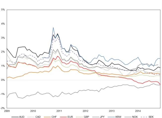
The two building blocks of our empirical analysis are the currencies’ quanto-implied risk premia (QRP, which measure the risk-neutral covariances between each currency and the S&P 500 index, as shown in equation (13)), and their interest rate differentials vis-`a-vis the US dollar (IRD, which would equal expected exchange rate appreciation if UIP held). Our measure of expected currency appreciation (the quanto forecast, or ECA) is equal to the sum of IRD and QRP, as in equation (14).
Figure 1 plots each currency’s QRP over time; for clarity, the figure drops two currencies for which we have highly incomplete time series (PLN and DKK). The QRP is negative for JPY and positive for all other currencies (with the partial exception of EUR, for which we observe a sign change in QRP near the end of our time period).
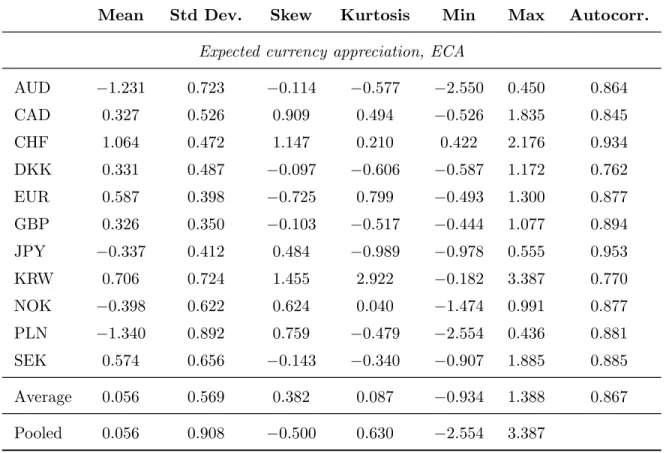
Figure IA.6 shows the evolution over time of ECA (solid) and of the UIP forecast (dashed) for each of the currencies in our panel. The gap between the two lines for a given currency is that currency’s QRP. Table 1 reports summary statistics of ECA. The penultimate line of the table averages the summary statistics across currencies; the last line reports summary statistics for the pooled data. Table 2 reports the same statistics for IRD and QRP.
The volatility of QRP is similar to that of interest rate differentials, both currency-by-currency and in the panel. There is considerably more variability in IRD and QRP when we pool the data than there is in the time series of a typical currency: this reflects substantial dispersion in IRD and QRP across currencies that is captured in the pooled measure but not in the average time series.
Table 3 reports volatilities and correlations for the time series of individual curren-cies’ ECA, IRD, and QRP. The table also shows three aggregated measures of volatil-ities and correlations. The row labelled “Time series” reports time-series volatilvolatil-ities and correlations for a typical currency, calculated by averaging time-series volatilities and correlations across currencies. Conversely, the row labelled “Cross section” re-ports cross-currency volatilities and correlations of time-averaged ECA, IRD, and QRP. Lastly, the row labelled “Pooled” averages on both dimensions: it reports volatilities and correlations for the pooled data.
All three variables (ECA, IRD, and QRP) are more volatile in the cross section than in the time series. This is particularly true of interest rate differentials, which exhibit far more dispersion across currencies than over time.
−0.696). Given the sign convention on IRD, this indicates that currencies with high in-terest rates (relative to the dollar) tend to have high risk premia; thus the predictions of the quanto theory are consistent with the carry trade literature and the findings of Lustig, Roussanov and Verdelhan (2011). The average time-series (i.e., within-currency) correlation between IRD and QRP is more modestly negative (ρ=−0.331): a typical currency’s risk premium tends to be higher, or less negative, at times when its interest rate is high relative to the dollar, but this tendency is fairly weak. The dis-parity between these two facts is accounted for by the strongly negative cross-sectional correlation between IRD and QRP (ρ=−0.798). If we interpret the data through the lens of Result 2, these findings suggest that the returns to the carry trade are more the result of persistentcross-sectional differences between currencies than of atime-series
relationship between interest rates and risk premia. This prediction is consistent with the empirical results documented by Hassan and Mano (2016).
We see a corresponding pattern in the time-series, cross-sectional, and pooled cor-relations of ECA and QRP. The time-series (within-currency) correlation of the two is substantially positive (ρ = 0.393), while the cross-sectional correlation is negative (ρ =−0.305). In the time series, therefore, a rise in a given currency’s QRP is asso-ciated with a rise in its expected appreciation; whereas in the cross-section, currencies with relatively high QRP on average have relatively low expected currency apprecia-tion on average (reflecting relatively high interest rates on average). Putting the two together, the pooled correlation is close to zero (ρ=−0.026). That is, Result 2 predicts that there should be no clear relationship between currency risk premia and expected currency appreciation; again, this is consistent with the findings of Hassan and Mano (2016).
These properties are illustrated graphically in Figure 2. We plot confidence ellipses centred on the means of QRP and IRD in panel (a), and of QRP and ECA in panel (b), for each currency. The sizes of the ellipses reflect the volatilities of IRD and QRP (or ECA): under joint normality, each ellipse would contain 50% of its currency’s ob-servations in population. (Our interest is in the relative sizes of the ellipses: the choice of 50% is arbitrary.) The orientation of each ellipse illustrates the within-currency time series correlation, while the positions of the different ellipses reveal correlations across currencies. The figures refine the discussion above. QRP and IRD are nega-tively correlated within currency (with the exceptions of CAD, CHF, and KRW) and
in the cross-section. QRP and ECA are positively correlated in the time series for every currency, but exhibit negative correlation across currencies; overall, the pooled correlation between the two is close to zero.
Our empirical analysis focuses on contracts with a maturity of 24 months because these have the best data availability. But in one case—the S&P 500 index quantoed into euros—we observe a range of maturities, so can explore the term structure of QRP. Figure IA.7 plots the time series of annualized euro-dollar QRP for horizons of 6, 12, 24, and 60 months. On average, the term structure of QRP is flat over the sample period, but QRP is slightly more volatile at shorter horizons, so that the term structure is downward-sloping when QRP spikes and upward-sloping when QRP is low.
2.1
A consistency check
Our data also includes quanto forward prices of certain other stock indexes, notably the Nikkei, Euro Stoxx 50, and SMI. We can use this data to explore the predictions of Section 1.2, which provides a consistency check on our empirical strategy.
Figure 3 implements (15) and (16) for the EUR-USD, JPY-USD, EUR-JPY, and EUR-CHF currency pairs. In each of the top-left, bottom-left and bottom-right panels, the solid line depicts the expected appreciation of the euro against the US dollar, yen, and Swiss franc, respectively, while the dashed line shows the expecteddepreciation of the three currencies against the euro (that is, we flip the sign on the “inverted” series for readability). In the top-right panel, the solid and dashed lines show the expected appreciation of the yen against the US dollar and expected depreciation of the US dollar against the yen, respectively. In every case, the two measures are strongly correlated over time and the solid line is above the dashed line, as they should be according to (18). The gaps between the measures are therefore consistent with the Jensen’s inequality correction one would expect to see if our currency forecasts measured expected currency appreciation perfectly. Moreover, given that annual exchange rate volatilities are on the order of 10%, the sizes of the gaps between the measures are quantitatively consistent with the Jensen’s inequality correction derived at the end of Section 1.2.
The EUR-CHF pair in the bottom-right panel represents a particularly interesting case study. The Swiss national bank instituted a floor on the EUR-CHF exchange rate at CHF1.20/e in September 2011 and consequently also reduced the conditional volatility of the exchange rate. Following this, the two lines converge and the gap stays
very narrow at around 0.2% up until January 2015, when the sudden removal of the floor prompted a spike in the volatility of the currency pair, visible in the figure as the point at which the two lines diverge.
2.2
Return forecasting
We run two sets of panel regressions in which we attempt to forecast, respectively, currency excess returns and currency appreciation. The literature on exchange rate forecasting has found it substantially more difficult to forecast pure currency apprecia-tion than currency excess returns, so the second set of regressions should be considered more empirically challenging. In each case, we test the prediction of Result 2 via pooled panel regressions. We also report the results of panel regressions with cur-rency fixed effects; by doing so, we allow for the more general possibility that there is a currency-dependent—but time-independent—component in the second covariance term that appears in the identity (6).
To provide a sense of the data before turning to our regression results, Figures 4 and 5 represent our baseline univariate regressions graphically in the same manner as in Figure 2. Figure 4 plots realized currency excess returns (RXR) against QRP and against IRD.11 Excess returns are strongly positively correlated with QRP both within
currency and in the cross-section, suggesting strong predictability with a positive sign. The correlation of RXR with IRD is negative in the cross-section but close to zero, on average, within currency.
Figure 5 shows the corresponding results for realized currency appreciation (RCA). Panel (a) suggests that the within-currency correlation with the quanto predictor ECA is predominantly positive (with the exceptions of AUD and CHF), as is the cross-sectional correlation. In contrast, panel (b) suggests that the correlation between realized currency appreciation and interest rate differentials is close to zero both within and across currencies, consistent with the view that interest rate differentials do not help to forecast currency appreciation.
We first run a horse race between the quanto-implied risk premium and interest
11As noted in Section 1, we work with true returns as opposed to log returns. Engel (2016) points
out that it may not be appropriate to view log returns as approximating true returns, since the gap between the two is a similar order of magnitude as the risk premium itself.
rate differential as predictors of currency excess returns: ei,t+1 ei,t − R $ f,t Ri f,t
=α+βQRPi,t +γIRDi,t+εi,t+1. (19)
Here (and from now on) the length of the period fromt tot+ 1 over which we measure our return realizations is 24 months, corresponding to the forecasting horizon dictated by the maturity of the quanto contracts we observe in our data.
We also run two univariate regressions. The first of these,
ei,t+1 ei,t − R $ f,t Ri f,t =α+βQRPi,t+εi,t+1, (20)
is suggested by Result 2. The second uses interest rate differentials to forecast currency excess returns, as a benchmark:
ei,t+1 ei,t −R $ f,t Ri f,t
=α+γIRDi,t+εi,t+1. (21)
We also run all three regressions with currency fixed effects αi in place of the shared
interceptα.
Table 4 reports the results. We report coefficient estimates and R2 for each
regres-sion, with and without currency fixed effects; standard errors are shown in parentheses. These standard errors are computed via a nonparametric bootstrap to account for het-eroskedasticity, cross-sectional and serial correlation in our data. (The serial correlation arises due to overlapping observations: we make forecasts of 24-month excess returns at monthly intervals.) For comparison, these nonparametric standard errors exceed those obtained from a parametric residual bootstrap by up to a factor of 2, and Hansen– Hodrick standard errors by a factor of around 1.3. We provide a detailed description of our bootstrap procedure and address potential small-sample concerns in Section 2.6.
The estimated coefficient on the quanto-implied risk premium is positive and eco-nomically large in every specification in which it occurs. Moreover, theR2 values are
substantially higher in the two regressions (19) and (20) that feature the quanto-implied risk premium than in the regression (21) in which it does not occur. The estimate forβ
in our headline regression (20) is 2.604 (standard error 1.127) in the pooled regression and 4.995 (standard error 1.565) in the regression with fixed effects. The fact that these
estimates are above 1 raises the possibility that beyond its direct importance in (6), the quanto-implied risk premium may also proxy for the second covariance term.12 We explore this issue in Section 2.5. Another noteworthy qualitative feature of our results is the consistently negative intercept, which reflects an unexpectedly strong dollar over our sample period; we discuss the statistical interpretation of this fact in Section 2.6.
Following Fama (1984), we can also test how the theory fares at predicting currency appreciation (ei,t+1/ei,t −1). To do so, we run the regression
ei,t+1 ei,t
−1 =α+βQRPi,t +γIRDi,t+εi,t+1. (22)
We do so not because we are interested in the coefficient estimates, which are mechan-ically related to those of regression (19), but because we are interested in the R2.
To explore the relative importance of the quanto-implied risk premium and interest rate differentials for forecasting currency appreciation, we run univariate regressions of currency appreciation onto the quanto-implied risk premium,
ei,t+1 ei,t
−1 =α+βQRPi,t+εi,t+1, (23)
and onto interest rate differentials,
ei,t+1 ei,t
−1 = α+γIRDi,t +εi,t+1. (24)
As previously, we also run the three regressions (22)–(24) with fixed effects.
The regression results are shown in Table 5, which is structured similarly to Table 4. There is little evidence that the interest rate differential helps to forecast currency appreciation on its own; this is consistent with the previous set of results and with the large literature that documents the failure of UIP. In the pooled panel, the estimated
γ in regression (24) is close to 0, and the R2 is essentially zero. With fixed effects, the estimate of γ is marginally negative, providing weak evidence that currencies tend to
12Another possibility is that it is more reasonable to think of a log investor as wishing to hold a
levered position in the market (sow >1 in the notation of footnote 7). If so, we should find a coefficient on QRP that is larger than one. We are cautious about suggesting this as an explanation, however, because a log investor would never risk bankruptcy. To match the point estimate for specification (20), we would need w = 2.604 or w = 4.995 (respectively without and with fixed effects). In the latter case, the investor would go bankrupt if the market dropped by 20% over the two year horizon.
appreciate against the dollar when their interest rate relative to the dollar is higher than its time-series mean.
More strikingly, the quanto-implied risk premium makes a very large difference in terms ofR2, which increases by two orders of magnitude when moving from
specifica-tion (24) to (22) in both the pooled regressions (0.16% to 16.01%) and the fixed-effects regressions (0.20% to 20.56%). It is also interesting that when QRP is included in the regressions (with or without fixed effects) the coefficient estimate on IRD,γ, increases toward the value of 1 predicted by Result 2.
For completeness, Table IA.5 reports the results of running regressions (20), (21), (22), and (24) separately for each currency at the 24-month horizon, and at 6- and 12-month horizons for the euro. Consistent with the previous literature (for example Fama (1984) and Hassan and Mano (2016)), the coefficient estimates are extremely noisy. A further appealing feature of Result 2 is that it provides a justification for constraining all the coefficient on the quanto-implied risk premium to be equal across currencies, as we have done above.
2.3
Risk-neutral covariance vs. true covariance
We have emphasized the importance of risk-neutral covariances of currencies with stock returns, as captured by quanto-implied risk premia, and below we will show that risk-neutral covariance performs well empirically. But it is natural to wonder whether this empirical success merely reflects the fact that currency returns line up with true co-variances, as studied by Lustig and Verdelhan (2007), Campbell, Medeiros and Viceira (2010), Burnside (2011) and Cenedese et al. (2016), among others. More formally, from the perspective of the log investor we can conclude, from (3), that
Et ei,t+1 ei,t − R $ f,t Ri f,t =R$f,tcovt ei,t+1 ei,t ,− 1 Rt+1 . (25)
Note that it is the true, not the risk-neutral, covariance that appears in this equation. The fundamental challenge for a test of this prediction is that forward-looking true covariance is not directly observed. This is the major advantage of our approach: risk-neutral covariance is directly observed via the quanto-implied risk premium. That said, we attempt to test (25) by using lagged realized covariance, RPCL, as a proxy for true forward-looking covariance.
The results are shown in Table 6 of the Appendix. RPCL is positively related to subsequently realized currency excess returns, as suggested by (25), but it is not statistically significant in our sample, and is driven out as a predictor by risk-neutral covariance (QRP), consistent with Result 2.
In principle, this might simply indicate that lagged realized covariance is an im-perfect proxy for true forward-looking covariance: perhaps the success of QRP simply reflects its superiority as a forecaster of realized covariance? Table 6 shows that risk-neutral covarianceis, individually, a statistically significant forecaster of future realized covariance. But it is driven out when lagged realized covariance and the interest-rate differential are included in the multivariate regression (31). Moreover, the optimal covariance forecast generated by this multivariate regression is driven out by QRP in the excess-return-forecasting regression (32).
The relationship between risk-neutral covariance and true covariance is interesting in its own right. Figure 6 illustrates the empirical relationship between the covariance forecast obtained from regression (31) (our proxy for forward-looking true covariance) and forward-looking risk-neutral covariance (obtained from quanto contracts). The two are positively correlated in the cross-section and in the time-series, but risk-neutral co-variance is generally larger (smaller) than future realized coco-variance for currencies with positive (negative) risk-neutral covariances. This is consistent with the observation of Lettau, Maggiori and Weber (2014) that carry trade returns are more correlated with the market at times of negative market returns. As we will now see, it is problematic for lognormal models.
2.4
Lognormal models
Lognormal models impose a tight connection between the covariance risk premium and the market and currency risk premium. Define the equity premium ERPt = logEt
Rt+1
R$f,t
and currency risk premium CRPi,t = logEt e Ri,t+1
R$
f,t
where Rei,t+1 = Rif,tei,t+1/ei,t is the
return on the currency trade defined earlier.
Result 3(The covariance risk premium in lognormal models). Suppose that the market return, exchange rate, and SDF are conditionally jointly lognormal. Then we have
or equivalently
covt(rt+1,∆ei,t+1) = covt∗(rt+1,∆ei,t+1), (27)
where rt+1 = logRt+1 and ∆ei,t+1 = log(ei,t+1/ei,t).
Proof. See Appendix B.
Empirically, it is plausible that the right-hand side of (26) is positive for most currencies (the yen being a possible exception). But we find that the left-hand side is typically negative in our data. No lognormal model can match these patterns.
It is nonetheless an interesting exercise to see how the quanto risk premium (and the residual covariance term, which would be zero from the perspective of the log investor) behaves inside an equilibrium model. As QRP has a simple characterization in terms of risk-neutral covariance, this is an easy exercise to carry out in any equilibrium model; we suggest that it makes an interesting diagnostic for future generations of international finance models. In that spirit, we have calculated the currency risk premium, QRP, IRD and the residual covariance term within the model of Colacito and Croce (2011). The results are shown in Internet Appendix IA.B. We deviate from the symmetric baseline calibration of Colacito and Croce in order to generate a non-trivial currency risk premium. The comparative statics of their long-run risk model are such that our calibrations which yield a positive asymmetric currency risk premium generate positive risk-neutral covariance (QRP) and a positive residual. In this model, the residual covariance term therefore adds to the prediction of the quanto forecast, as opposed to offsetting it. This positive relationship between risk-neutral covariance and the residual is consistent with our finding that the slope coefficients on QRP in the predictive regressions in Section 2.2 are generally larger than 1.
2.5
Beyond the log investor
The identity (6) expresses expected currency appreciation as the sum of IRD, QRP, and a covariance term,−covt(Mt+1Rt+1, ei,t+1/ei,t). Thus far, we have either assumed that
this term is constant across currencies and over time (so is captured by the constant in our pooled regressions) or that it has a currency-dependent but time-independent component (so is captured by fixed effects).
To get a sense of what these assumptions may leave out, we conduct a principal components analysis on unexpected currency excess returns: that is, on the difference
between realized currency excess returns and the corresponding ex ante expected re-turns. We calculate these unexpected excess returns in two ways. Regression residuals
are defined as the estimated residuals εi,t+1 in the specification of regression (20) that
includes currency fixed effects. Theory residuals are defined similarly, except that we impose α= 0, β = 1 in (20).
These residuals reflect both the ex ante residual from the identity (6) and the ex post realizations of unexpected currency returns. The identity implies that the predictable component of the realized residuals—if there is one—reveals the covariance term,−covt(Mt+1Rt+1, ei,t+1/ei,t).
We decompose the theory and regression residuals into their respective principal components (dropping DKK, KRW, and PLN from the panel to minimize the impact of missing observations). Table IA.2 shows the principal component loadings. The first principal component, which explains just under two thirds of the variation in residuals, can be interpreted as a level, or ‘dollar,’ factor since it loads positively on all currencies (with the exception of GBP, in the case of the regression residuals).
Motivated by this fact, we now include an additional predictor variable, IRDt,
which is calculated as the cross-sectional average of the interest rate differentials in our balanced panel of eight currencies (i.e., excluding DKK, KRW, and PLN); Lustig, Roussanov and Verdelhan (2014) interpret this average interest rate differential (which they refer to as the ‘average forward discount’) as a dollar factor and show that it helps to forecast currency returns. We also include the logarithm of the real exchange rate, which Dahlquist and Penasse (2017) have shown to be a successful forecaster of currency returns.
Table 7 reports the results of regressions of currency excess returns onto currency fixed effects and subsets of four forecasting variables: the quanto-implied risk premium (QRP), the interest rate differential (IRD), the real exchange rate (RER), and the average interest rate differential (IRD). The table reports the univariate, bivariate, 3-variate, and 4-variate specifications with the highest R2. (Table IA.3 reports the R2
for all 24 −1 = 15 subsets of the four explanatory variables, though not—for lack of
space—the estimated coefficients.) The quanto-implied risk premium features in all
R2-maximizing regressions. The estimates of β are larger than 1 in every specification,
suggesting that, over and above its relevance as a direct measure of risk-neutral covari-ance, the quanto-implied risk premium helps to capture the physical covariance term
in (6). As we increase from one to two to three explanatory variables, R2 increases from 22.03% (using QRP alone) to 35.40% (adding the real exchange rate) to 43.56% (adding the dollar factor IRD). The interest rate differential itself, IRD, contributes almost no further explanatory power when it is then added as a fourth variable.
As the real exchange rate performs well, we report further results relating to it in Table IA.4 of the Internet Appendix.
2.6
Joint hypothesis tests and finite-sample issues
We now consider the joint hypothesis tests that are suggested by Result 2. In our three main specifications (19), (20), and (22), equation (14) predicts an interceptα = 0, and a slope coefficient on QRP β = 1. For the excess return forecast in regression (19), it predicts that the interest rate differential should have no predictive power, i.e. γ = 0; whereas it predicts thatγ = 1 in the currency-appreciation regression (22).
Here, as elsewhere, we use a nonparametric bootstrap procedure to compute the co-variance matrix of coefficient estimates. A detailed exposition of the bootstrap method-ology is provided in Politis and White (2004) and Patton, Politis and White (2009). In the bootstrap procedure, we resample the data by drawing with replacement blocks of 24 time-series observations from the panel while ensuring that this time-series resam-pling is synchronized in the cross-section. The length of the time-series blocks is chosen to equal the forecasting horizon of 24 months. The resulting panel is then resampled with replacement in the cross-sectional dimension by drawing blocks of uniformly dis-tributed width (between 2 and 11, the latter being the width of the full cross-section). Since currencies which are adjacent in the panel are more likely to be included to-gether in any given one of these cross-sectional blocks, we permute the cross-section of our panel randomly before each resampling. We then compute the point estimates of the coefficients from the two-dimensionally resampled panel and repeat this procedure 100,000 times. The standard errors are then computed as the standard deviations of the respective coefficients across the 100,000 bootstrap repetitions.
Table 8 reports p-values for tests of various hypotheses about our baseline re-gressions. In addition to conventional p-values calculated using the asymptotic (chi-squared) distribution of the Wald test statistic, the table also reports more conser-vative small-sample p-values obtained from a bootstrapped test statistic distribution. We compute these small-sample p-values by constructing a small-sample distribution
of the Wald test-statistic for each regression: We simulate 5,000 sets of monthly data for the LHS variable under the null hypothesis of no predictability, such that the simu-lated data matches the monthly autocorrelation and covariance matrix of the realized, observed LHS data. We then aggregate the simulated monthly data into 24-month horizon data, like the LHS data used in our regressions (e.g. excess returns over 24 months). As we aim to measure the small-sample performance of our bootstrap rou-tine, the simulated data sets each have the same number of data points as the observed LHS data. For each specification, we then regress the 5,000 simulated LHS data on the respective observed RHS variable(s). Where we run the regression with currency fixed effects, we use the demeaned RHS variable(s). We obtain the point estimates of the coefficients and their covariance matrix from the bootstrap routine outlined above and use the test statistics from these 5,000 regressions to construct the empiri-cal small-sample distribution of the respective Wald statistic under the respective null hypothesis. This procedure also accounts for the potential small-sample Stambaugh bias in the p-values.
Figure IA.8 illustrates by plotting the histograms of the bootstrapped distribution of test statistics for various hypotheses on regression (22). Panels a and b show the finite-sample bootstrapped distributions of the test statistic for the hypothesis that Result 2 holds, respectively in the pooled and fixed-effects regressions. The value of the test statistic in the data is indicated with an asterisk in each panel. The finite-sample and asymptotic (shown with a solid line) distributions are strikingly different: the asymptotic distribution suggests that we can reject the hypothesis that Result 2 holds, but this conclusion is overturned by the finite-sample distribution. (In the pooled case, the discrepancy is largely due to the intercept, as becomes clear on comparing the asymptoticp-values for tests of hypothesesH1
0 and H02 in Table 8: the asymptotic
distribution penalizes the fact that the US dollar was strong over our sample period, whereas the finite-sample distribution does not.)
In contrast, the asymptotic and finite-sample distributions tell more or less the same story in panels c and d, which show the corresponding results for tests (without and with fixed effects) of the hypothesis H3
0 that β = 0, i.e. that QRP is not
use-ful in forecasting currency appreciation. While the small-sample distributions of the test statistics exhibit fatter tails than the asymptoticχ2 distribution, the discrepancy between the two is small by comparison with panels a and b, and even using the
finite-sample distribution we can reject the hypothesis with some confidence (with p-values of 0.082 and 0.051 in the pooled and fixed-effects cases, respectively).
We reach similar conclusions for regressions (19) and (20): we do not reject the predictions of Result 2 in the joint Wald tests for any of the three baseline regressions using the small-sample distribution of the test statistic; and QRP remains individually significant as a predictor at the 10% level in all three specifications, with and without currency fixed effects, even if we take the most conservative approach to computing
p-values that relies on the empirical small-sample test statistic distribution.
3
Out-of-sample prediction
We now test the quanto theory out of sample. Since the dollar strengthened strongly over the relatively short time period spanned by our data (as reflected in the negative intercept in our pooled panel regression (22)), we focus on forecasting differential cur-rency appreciation: that is, we seek to predict, for example, the relative performance of dollar-yen versus dollar-euro.
In the previous section, we estimated the loadings on the quanto-implied risk pre-mium, QRP, and interest rate differential, IRD, via panel regressions. These deliver the best in-sample coefficient estimates in a least-squares sense. But for an out-of-sample test we must pick the loadings a priori. Here we can exploit the distinctive feature of Result 2 that it makes specific quantitative predictions for the loadings: each should equal 1, as in the formula (14). We therefore compute out-of-sample forecasts by fixing the coefficients that appear in (22) at their theoretical values: α= 0, β = 1, γ = 1.
We compare these predictions to those of three competitor models: UIP (which predicts that currency appreciation should offset the interest rate differential, on aver-age), a random walk without drift (which makes the constant forecast of zero currency appreciation, and which is described in the survey of Rossi (2013) as “the toughest benchmark to beat”), and relative purchasing power parity (which predicts that cur-rency appreciation should offset the inflation differential, on average). These models are natural competitors because, like our approach, they make a priori predictions without requiring estimation of parameters, and so avoid in-sample/out-of-sample issues.
define a dollar-neutralR2-measure similar to that of Goyal and Welch (2008): ROS2 = 1− P i P j P t(ε Q i,t+1−ε Q j,t+1)2 P i P j P t(ε B i,t+1−εBj,t+1)2 ,
where εQi,t+1 and εB
i,t+1 denote forecast errors (for currency i against the dollar) of the
quanto theory and the benchmark, respectively, so our measure compares the accuracy of differential forecasts of currencies i and j against the dollar. We hope to find that the quanto theory has lower mean squared error than each of the competitor models, that is, we hope to find positiveR2
OS versus each of the benchmarks.
The results of this exercise are reported in Table 9. The quanto theory outperforms each of the three competitors: when the competitor model is UIP, we find thatR2
OS =
10.91%; and when it is relative PPP, we find R2
OS = 26.05%. In our sample, the
toughest benchmark is the random walk forecast, consistent with the findings of Rossi (2013). Nonetheless, the quanto theory easily outperforms it, with R2OS = 9.57%.
To get a sense for whether our positive results are driven by a small subset of the currencies, Table 9 also reports the results of splitting the R2 measure
currency-by-currency: for each currencyi, we define
ROS,i2 = 1− P j P t(ε Q i,t+1−ε Q j,t+1)2 P j P t(ε B i,t+1−εBj,t+1)2 .
This quantity is positive for all i and all competitor benchmarks B, indicating that the quanto theory outperforms all three benchmarks for all 11 currencies. We run Diebold–Mariano tests (Diebold and Mariano, 1995) of the null hypothesis that the quanto theory and competitor models perform equally well for all currencies, using a small-sample adjustment proposed by Harvey, Leybourne and Newbold (1997), and find that the outperformance is strongly significant.
Jord`a and Taylor (2012) have argued that assessments of forecast performance based solely on mean squared errors may not fully reflect the economic benefits of a forecasting model. In Appendix IA.A, we use the approach they suggest, which essentially asks whether a predictor variable is more or less successful at predicting whether a currency will appreciate or depreciate than competitor predictors. (This is an oversimplification; full details are in Appendix IA.A.) Our approach also outperforms on their metric, both in forecasting currency excess returns and in forecasting currency appreciation.
4
Conclusion
UIP forecasts that high interest rate currencies should depreciate on average: it re-flects the expected currency appreciation that a genuinely risk-neutral investor would perceive in equilibrium. Unsurprisingly—given that the financial economics literature has repeatedly documented the importance of risk premia—the UIP forecast performs extremely poorly in practice.
We have proposed an alternative forecast, the quanto-implied risk premium, that can be interpreted as the expected excess return on a currency perceived by an investor with log utility whose wealth is fully invested in the stock market. Like the UIP forecast, the quanto forecast has no free parameters and can be computed directly from asset prices. Unlike the UIP forecast, the quanto forecast performs well empirically both in and out of sample. Its main deficiency is its failure to predict the strength of the dollar itself on average against other currencies over our sample period: time will tell if this is a small-sample issue or something more fundamental.
We find that currencies tend to have high quanto-implied risk premia if they have high interest rates on average, relative to other currencies (a cross-sectional statement), or if they currently have unusually high interest rates (a time-series statement); and that there is more cross-sectional than time-series variation in quanto-implied risk premia. These facts explain both the existence of the carry trade and the empirical importance of persistent cross-currency asymmetries, as documented by Hassan and Mano (2016).
The interpretation of the quanto-implied risk premium as revealing the log investor’s expectation of currency excess returns is a special case of the identity (6), which de-composes expected currency appreciation into the interest rate differential (the UIP term), risk-neutral covariance (the quanto-implied risk premium), and a real-world co-variance term that, we argue, is likely to be small—and in particular, smaller than the corresponding covariance term in the well-known identity (3). In the log investor case, this real-world covariance term is exactly zero, a fact we use to provide intuition and to motivate our out-of-sample analysis. But we also allow for deviations from the log investor benchmark—that is, for a nontrivial real-world covariance term—by running regressions including currency fixed effects, realized covariance, interest rate differen-tials, the average forward discount of Lustig, Roussanov and Verdelhan (2014), and the real exchange rate, as in Dahlquist and Penasse (2017), in addition to the