Alexander Hapfelmeier
Random Forest variable importance with missing
data
Technical Report Number 121, 2012
Department of Statistics
University of Munich
Random Forest variable importance with missing data
Alexander Hapfelmeier
Institut f¨ur Medizinische Statistik und Epidemiologie, Technische Universit¨at M¨unchen,
Ismaninger Str. 22, 81675 Munich, Germany, [email protected]
Kurt Ulm
Institut f¨ur Medizinische Statistik und Epidemiologie, Technische Universit¨at M¨unchen,
Ismaninger Str. 22, 81675 Munich, Germany
Torsten Hothorn
Institut f¨ur Statistik, Ludwig-Maximilians-Universit¨at, Ludwigstraße 33, 80539 Munich, Germany
February 15, 2012
Abstract
Random Forests are commonly applied for data prediction and interpretation. The latter purpose is supported by variable importance measures that rate the relevance of predictors. Yet existing measures can not be computed when data contains missing values. Possible solutions are given by imputation methods, complete case analysis and a newly suggested importance measure. However, it is unknown to what extend these approaches are able to provide a reliable estimate of a variables relevance. An extensive simulation study was performed to investigate this property for a variety of missing data generating processes. Findings and recommendations: Complete case analysis should not be applied as it inappropriately penalized variables that were completely observed. The new importance measure is much more capable to reflect decreased information exclusively for variables with missing values and should therefore be used to evaluate actual data situations. By contrast, multiple imputation allows for an estimation of importances one would potentially observe in complete data situations.
Keywords: Random Forests, variable importance measures, missing data, multiple imputation, surrogates, complete case analysis
1
Introduction
Random Forests (cf. Breiman, 2001) are popular ap-proaches for regression analysis. On account of their easy applicability and interpretability they are com-monly used in many research fields such as social, econometric and clinical science. Further strong ad-vantages over common approaches like regression anal-ysis are their ability to implicitly deal with high dimen-sional data, missing values, complex interactions and collinearity (cf. Cutler et al., 2007; Lunetta et al., 2004, for corresponding discussions). Likewise, Random Forests provide variable importance measures which can be used to identify variables that are of relevance for prediction. In a subsequent step these measures are often used for variable selection (cf. Tang et al., 2009; Yang and Gu, 2009; Rodenburg et al., 2008; Sandri and Zuccolotto, 2006; D´ıaz-Uriarte and Alvarez de Andr´es, 2006; Altmann et al., 2010; Archer and Kimes, 2008). So far, it has not been investigated how to proceed for the computation of such measures when there is
missing data. Complete case analysis and imputation (e.g. mean, hot-deck, conditional mean and predic-tive distribution substitution) are two potential solu-tions to this issue. However, it has been shown that these ad hoc methods may lead to biased inference when the data is not missing completely at random (cf. Schafer and Graham, 2002; Horton and Klein-man, 2007). Multiple imputation by chained equations (MICE; cf. van Buuren et al., 2006; White et al., 2011) is meant to solve this problem and its superiority has been shown in many publications (e.g. Janssen et al., 2009, 2010). A third solution has been proposed ear-lier (cf. Hapfelmeier et al., 2012) by a new variable importance measure. It is closely related to existing approaches – and therefore retains appreciated prop-erties – yet handles missing values in an intuitive way. The predictive accuracy of Random Forests has been explored for the analysis of missing data by Rieger et al. (2010); Hapfelmeier et al. (2011): comparisons of models fit with and without imputation of missing values showed only negligible differences. By contrast,
the following study focuses on the assessment of a vari-ables relevance by means of importance measures. As a result the ability to produce reliable estimates well differs between complete case analysis, multiple impu-tation (executed by MICE) and the new importance measure. An extensive simulation study that involves various missing data generating processes is conducted for both, regression and classification problems. Find-ings about predictive accuracy are retraced in an ad-ditional analysis of a simulated test dataset.
2
Missing Data
In early works Rubin (1976, 1987) specifies the issue of correct statistical inference with missing values by the definition of missing data generating processes:
• Missing completely at random (MCAR):
P(R|Xcomp) =P(R)
• Missing at random (MAR):
P(R|Xcomp) =P(R|Xobs)
• Missing not at random (MNAR):
P(R|Xcomp) =P(R|Xobs,Xmis)
Whether a value is missing is indicated by a binary variableR and depends on its probability distribution
P(R). The complete variable set Xcomp consists of the observed values Xobs and the missing ones Xmis: Xcomp={Xobs,Xmis}. Therefore in a MCAR scheme the probability for a missing value is independent of the observed and unobserved data. By contrast for MAR this probability is dependent on the observed information. In MNAR the probability depends on unobserved variables or the missing values themselves. Little and Rubin (2002) showed that usual sample estimates – for example in linear regression – stay un-affected by the MCAR scheme. By contrast, in classi-fication and regression trees even MCAR may induce a systematic bias, that may be carried forward to Ran-dom Forests based on biased split selections (cf. Strobl et al., 2007). Also, it is well-known that complete case analysis is prone to biased inference when the data is not MCAR. Therefore, in the following simulation study, one MCAR, four MAR and one MNAR scheme to generate missing values are investigated.
3
Methods
3.1
Random Forests
The most famous representative of recursive partition-ing is the CART algorithm (cf. Breiman et al., 1984). It constructs trees by sequential binary splits that pro-duce subsets of the data which are as homogeneous as possible in terms of the outcome. Breiman (1996)
also showed that the performance of single trees ben-efits from “bagging” (bootstrap aggregation). In bag-ging, several trees are fit to bootstrapped or subsam-pled data. As a further advancement, Random Forests (Breiman, 2001; Breiman and Cutler, 2008) have been introduced for which splits are performed in random selections of variables. This makes a more diverse set of variables contribute to the joint prediction. The latter is found by averaged values or majority votes of each single tree in a Random Forest. The so called ‘out of bag’ (OOB) samples – i.e. observations not used to fit the respective trees – can be used for an unbiased estimate of a Random Forests error, viz. the OOB-error.
When there are missing values surrogate splits need to be employed. They mimic the initial split of the data as they try to archive the same partitioning of complete observations. When several surrogate splits are computed they can be ranked according to their ability to resemble the initial split. An observation that contains more than a single missing value is pro-cessed along this ranking until a decision is found.
The CART and the C4.5 algorithms – and conse-quently all Random Forest algorithms based on the same construction principles – have been shown to be prone to biased variable selection (cf. Breiman et al., 1984; Strobl et al., 2007; White and Liu, 1994; Kim and Loh, 2001; Dobra and Gehrke, 2001; Hothorn et al., 2006). Therefore, Random Forests used in this work base on the recursive partitioning approach of Hothorn et al. (2006). It follows the same rationale as Breiman’s original approach and guarantees unbiased variable se-lection and variable importance measures when com-bined with subsampling (as opposed to bootstrap sam-pling; cf. Strobl et al., 2007).
3.2
A new variable importance
mea-sure for missing data
The most popular and most advanced variable impor-tance measure for Random Forests is the permutation accuracy importance. It is assessed by a comparison of a trees prediction accuracy before and after the random permutation of a predictor variable. If the latter is of relevance the accuracy is supposed to drop as the orig-inal association to the response and further predictors is destroyed by permutation; the importance measure takes large values in such a case. The major issue is that there is no straightforward way to compute this measure when there are missing values. In particular, it is not clear how conclusions about the importance of variables can be drawn from the permutation approach when surrogate splits are involved in the computation of the accuracy.
A new approach was proposed earlier (cf. Hapfelmeier et al., 2012) to overcome this pit-fall. In order to retain appreciated properties it is closely related to existing methodology, yet differs
in one substantial aspect: Instead of permuting the values of a variable X (that may be missing), observations are randomly send to the daughter nodes if a parent node k is split in X. The probability to be sent left is determined by the relative frequency
ˆ
pk of observations that initially went this way. The
algorithm to compute the new importance measure is given by:
1. Compute the OOB accuracy of a tree.
2. Randomly assign each observation with ˆpk to the
left (or right) child node if the parent node k is split inX.
3. Recompute the OOB accuracy of the tree. 4. Compute the difference between the original and
recomputed OOB accuracy.
5. Repeat step 1 to 4 for each tree and use the aver-age difference over all trees as the overall impor-tance score.
This procedure simulates – like for the random per-mutation in the original perper-mutation importance – the null hypothesis that the allocation of observations does not depend on the particular predictor variable. It solves any problems associated with the occurrence of missing values and the application of surrogate splits as decisions are detached from the raw values of a vari-able.
3.3
Multivariate
Imputation
by
Chained Equations
Single imputation can lead to severe underestimation of variance (cf. Harel and Zhou, 2007). A simple and popular solution to this problem is the application of multiple imputation (MI; cf. Rubin, 1987, 1996). In a first step a proper MI approach is supposed to draw M estimates θ(1), ..., θ(M) from P(θ|X
obs) for the multi-dimensional parameter θ which determines the data distribution. These are subsequently used in the con-ditional distributions P(Xmis|Xobs;θb(t)), t = 1, ...,M to draw multiple imputations for missing values. This way several imputed datasets are created. Finally, any measure of interest can be assessed by the average of estimates for each of the imputed datasets. Little and Rubin (2002) point out that the approach makes stan-dard complete-data methods applicable to incomplete data (e.g. the original permutation importance mea-sure).
The case of more than one variable with missing val-ues demands for a special imputation procedure. A practical approach which makes it possible to bypass the specification of a joint distribution is MICE (some-times also called fully conditional specification (FCS); cf. van Buuren et al., 2006; van Buuren, 2007; van Buuren and Groothuis-Oudshoorn, 2010; White et al.,
2011). It cycles through incomplete variables to itera-tively update imputed values and parameter estimates until convergence. The procedure is repeated several times to produce multiple imputed data sets. An ap-parent advantage is that imputation of the data can be achieved by a flexible specification of predictive models for each variable.
MICE is especially suitable in MAR settings though Janssen et al. (2010) state that it should also be pre-ferred to ad hoc methods like complete case analysis even in MNAR situations. Likewise He et al. (2009) and White et al. (2011) point out that MICE is also capable to deal with MNAR schemes as the imputa-tion model becomes more general and includes more variables to make MAR plausible.
4
Simulation study
An extensive simulation study was designed to investi-gate the ability of complete case analysis, multiple im-putation by MICE and the new importance measure to produce reliable estimates of a variables relevance. In addition, the predictive accuracy of Random Forests that base on each of these approaches was explored for a simulated test dataset. There are several factors of potential influence that needed to be explored; there-fore the amount of missing values, correlation schemes, variable strength and different processes to generate missing values were of particular interest. A detailed explanation of the setup is given in the following.
• Influence of predictor variables
The simulated data contained both, a classifica-tion and a regression problem. Therefore, a cat-egorical (binary) and a continuous response were created in dependence of six variables with coeffi-cientsβ:
β= (1,1,0,0,1,0)>.
Repeated values forβmake it possible to compare importances of variables which are, by construc-tion, equally influential but show different correla-tions and different fraccorrela-tions of missing values. In addition, the non-influential variables withβ = 0 help to investigate possible undesired effects and serve as a baseline.
• Data generating models
A continuous response was modeled by means of a linear model:
y=x>β+with∼N(0, .5).
The binary response was drawn from a Bernoulli distributionB(1, π) withπwhich was assessed by means of a logistic model
π=P(Y = 1|X=x) = e x>β
The variable set X itself contained 100 observa-tions drawn from a multivariate normal distribu-tion with mean vector ~µ= 0 and covariance ma-trix Σ: • Correlation Σ = 1 0.3 0.3 0.3 0 0 0.3 1 0.3 0.3 0 0 0.3 0.3 1 0.3 0 0 0.3 0.3 0.3 1 0 0 0 0 0 0 1 0 0 0 0 0 0 1
As the variances of each variable are chosen to be 1, the covariance equals the correlation in this special case. The structure of Σ reveals that there is a block of four correlated variables and two un-correlated ones.
• Missing values
Several MCAR, MAR and MNAR processes to create missing values were implemented. For each scheme, a given fraction m ∈ {0.0,0.1,0.2,0.3} of values is set missing for the variables X2,
X4 and X5. The number of observations that contain at least one missing value is given by 1−(1−%missing)nvariables. Thus, a dataset that contains three variables with 30% missing values includes 1−(1−0.3)3= 65.7% incomplete obser-vations on average. This seems to be a rather huge amount though it is not unlikely for real life data. Therefore, m comprises a wide range of possible scenarios.
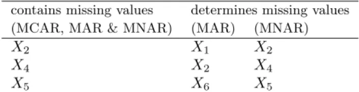
In the MAR setting, the probability for missing values in a variable depended on the values of an-other variable. In the MNAR scheme this proba-bility was determined by a variables own values. Accordingly, each variable that contained missing values had to be linked to at least one other vari-able or itself. Tvari-able 1 lists the corresponding re-lations.
Table 1: List of variables that contain missing values determine the probability of missing values.
contains missing values determines missing values (MCAR, MAR & MNAR) (MAR) (MNAR)
X2 X1 X2
X4 X2 X4
X5 X6 X5
The schemes to produce missing values are:
– MCAR: Values are randomly replaced by missing values.
– MAR(rank): The probability of a value to be replaced by a missing value rises with the rank the same observation has in the deter-mining variable.
– MAR(median): The probability of a value to be replaced by a missing value is nine times higher for observations whose value in the de-termining variable is located above the cor-responding median.
– MAR(upper): Those observations with the highest values of the determining variable are replaced by missing values.
– MAR(margins): Those observations with the highest and lowest values of the determining variable are replaced by missing values.
– MNAR(upper): The highest values of a vari-able are set missing.
An independent test dataset served the purpose to evaluate the predictive accuracy of a Random For-est. It was created the same way as the training data though it contained 5000 observations and was com-pletely observed. The accuracy was assessed by the mean squared error (MSE) which equals the misclassi-fication error rate (MER) in classimisclassi-fication problems.
In summary, there were 2 response types in-vestigated for 6 processes to generate and 3 pro-cedures to handle 4 different fractions of miss-ing values. This sums up to as much as 144 simulation settings. The simulation was repeated 1000 times. Corresponding R-Code is available online at http://www2.imse.med.tu-muenchen.de/ r-code/hapfelmeier/RF_VI_missingData.r.
5
Results
The following investigations are based on the classifi-cation analysis. Results for the regression problem are presented as supplementary material in section A (cf. Figure 5) as they showed similar properties.
A general finding which holds for each analysis ac-centuates the well-known fact that unconditional per-mutation importance measures rate the relevance of correlated variables higher than that of uncorrelated ones (cf. Strobl et al., 2008). This becomes evident by the example of variables 1, 2 and 5. Although they are of equal strength the latter is assigned a lower rel-evance as it is uncorrelated to any other predictor; in some research fields this effect is appreciated to un-cover relations and interactions among variables (cf. Nicodemus et al., 2010; Altmann et al., 2010). Also, there were no artificial effects observed for the non-influential variables in any analysis setting.
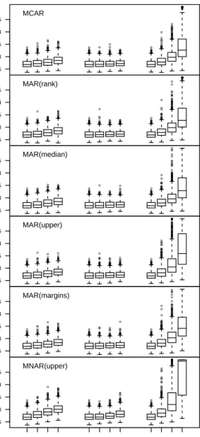
Findings for the new variable importance measure which is able to implicitly deal with missing values are displayed by Figure 1. According to expectations, the importance of variables 2, 4 and 5 decreased as they contained a rising amount of missing values. It is interesting to note that meanwhile the importance of variable 1 rose, although it does not seem to be directly affected. However, Hapfelmeier et al. (2012)
showed that this gain of relevance is justified: variables that are correlated and therefore provide similar infor-mation replace each other in a Random Forest when some of the information gets lost due to missing val-ues. Accordingly, variable 1 takes over for variable 2 which reflects in an increased selection frequency of variable 1 in the tree building process. In conclusion, this approach is allowed to be affected by the occur-rence of missing values as it mirrors the situation at hand, i.e. the relevance a variable takes in a Random Forest under consideration of the information it actu-ally provides. The new importance measure appeared to be well suited for any of the missing data generating processes as results did not differ substantially.
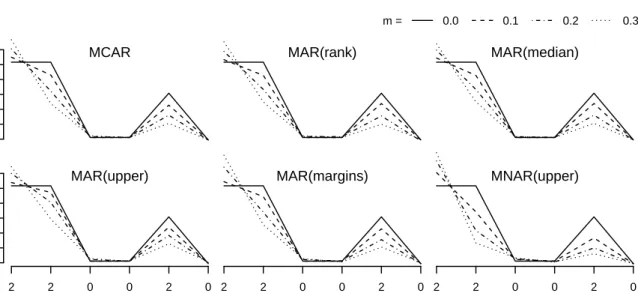
Results for the complete case analysis – given by Figure 2 – showed undesired effects. A rising amount of missing values lead to a decreased importance of the complete variable 1. This is due to the simple fact that some observations are completely discarded from analysis; importance measures typically diminish when Random Forests are fit to less data. However, its importance is not supposed to drop below that of variable 2 which is of equal strength yet contains the missing values. Unfortunately, this latter effect can be observed for every missing data generating process, except for MNAR(upper). It is most pronounced for MAR(upper) and MAR(margins). There is no ratio-nal justification for this property as variable 1 sustains its information while other variables loose it. A proper evaluation of a variables relevance is supposed to re-flect this fact. Considering this vulnerability of com-plete case analysis to different missing data generating processes it should not be used for the assessment of importance measures when there is missing data.
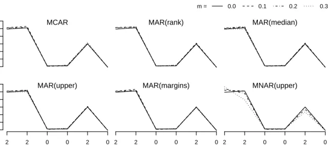
An examination of Figure 3 reveals that multiple im-putation – with only as few as five imputed data sets – is a convenient way to maintain and recover the im-portance of variables that would have been observed if there was no missing data at all. This equally held for variables that contained missing values and those which were completely observed; none of their impor-tances was arbitrarily decreased or increased. Even the importance of variable 5 which is only related to the outcome and therefore is associated with a rather weak imputation model remained unaffected by the amount of missing values. The example of variable 4 shows that the imputation of non-influential variables did not induce artificial importances. All missing data gener-ating processes showed these advantageous properties, except for the MNAR(upper) setting.
The prediction error produced by each approach for the independent test sample is displayed in Figure 4. For multiple imputation the prediction accuracy only slightly decreases with a rising amount of miss-ing values. This effect is more pronounced for Ran-dom Forests that use surrogate splits; though there are only minor differences to multiple imputation (cf. Rieger et al., 2010; Hapfelmeier et al., 2011, for
ac-● ● ● ● ● ● ● ● ● ● ● ● ● ● ● ● ● ● ● ● ● ● ● ● ● ● ● ● ●●●● ● ● ● ● ● ● ● ● ● ● ● ● ● ● ● ● ● ● ● ● ● ● ● ● ● ● ● ● ● ● ● ●●●● ● ● ● ● ●●● ● ● ● ● ● ● ● ● ● ● ● ●●● ● ● ● ● ● ● ● ● ● ● ● ● ● ●● ● ● ● ● ● ● ● ● ● ● ● ● ● ● ● ● ● ● ● ● ● ● ● ● ● ● ● ● ● ● ● ● ● ● ● ● ● ● ● ● ● ● ● ● ● ● ● ● ● ● ● ● ● ● ● ● ● ● ● ● ● ● ● ● ● ● ● ● ● ● ● ● ● ● ● ● ● ● ● ● ● ● ● ● ● ● ● ● ● ● ● ● ● ● ● ● ● ● ● ● ● ● ● ● ● ● ● ● ● ● ● ● ● ● ● ● ● ● ● ● ● ● ● ● ● ● ● ● ● ● ● ● ● ● ● ● ● ● ● ● ● ● ● ● ● ● ● ● ● ● ● ● ● ● ● ● ● ● ● ● ● ● ● ● ● 0.25 0.3 0.35 0.4 0.45 MCAR
new measure imputation complete case
● ● ● ● ● ● ● ● ● ● ● ● ● ● ● ● ● ● ● ● ● ● ● ● ● ● ● ● ● ● ● ● ● ● ● ● ● ● ● ● ● ● ● ● ● ● ● ● ● ● ● ● ● ● ● ● ● ● ● ● ● ●● ● ● ● ● ● ● ● ● ● ● ● ●● ● ● ● ● ● ● ● ● ● ● ● ● ● ● ● ● ● ● ● ● ● ● ● ● ● ● ● ● ●● ● ● ● ● ● ● ● ● ● ● ● ● ● ● ● ● ● ● ● ● ● ● ● ● ● ● ● ● ● ● ● ● ● ● ● ● ● ● ● ● ● ● ● ● ● ● ● ● ● ● ● ● ● ● ● ● ● ● ● ● ● ● ● ● ● ● ● ● ● ● ● ● ● ● ● ● ● ● ● ● ● ● ● ● ● ● ● ● ● ● ● ● ● ● ● ● ● ● ● ● ● ● ● ● ● ● ● ● ● ● ● ● ● ● ● ● ● ● ● ● ● ● ● ● ● ● ● ● ● ● ● ● ● ● ● ● ● ● ● ● ● ● ● ● ● ● ● ● ● ● ● ● ● ● ● ● ● ● ● ● ● ● ● ● ● 0.25 0.3 0.35 0.4 0.45 MAR(rank) ● ● ● ● ● ● ● ● ● ● ● ● ● ● ●●●● ● ● ● ● ● ●● ● ● ● ● ● ● ● ● ● ● ● ● ● ● ● ● ● ● ● ● ● ● ● ● ● ● ● ● ● ● ● ● ●●● ● ● ● ● ● ● ●●●●●● ● ● ● ● ● ● ● ● ● ● ● ● ● ● ● ● ● ● ● ● ● ● ● ● ● ● ● ● ● ● ● ● ● ● ● ● ● ● ● ● ● ● ● ● ● ● ● ● ● ● ● ● ● ● ● ● ● ● ● ● ● ● ● ● ● ● ● ● ● ● ● ● ● ● ● ● ● ● ● ● ● ● ● ● ● ● ● ● ● ● 0.25 0.3 0.35 0.4 0.45 MAR(median) ● ● ● ● ● ● ● ● ● ● ● ● ● ● ●● ● ● ● ● ● ● ● ●●● ● ● ● ● ● ● ● ● ● ● ● ● ● ● ● ● ● ● ● ● ● ● ● ● ● ● ● ● ● ● ● ● ● ● ● ●●● ● ● ● ● ● ● ● ● ● ● ● ● ● ● ● ● ● ● ● ● ● ● ● ● ● ● ● ● ● ● ● ● ● ● ● ● ● ● ● ● ● ● ● ● ● ● ● ● ● ● ● ● ● ● ● ● ● ● ● ● ● ● ● ● ● ● ● ● ● ● ● ● ● ● ● ● ● ● ● ● ● ● ● ● ● ● ● ● ● ● ● ● ● ● ● ● ● ● ● ● ● ● ● ● ● ● ● ● ● ● ● ● ● ● ● ● ● ● ● ● ● ● ● ● ● ● ● ● ● ● 0.25 0.3 0.35 0.4 0.45 MAR(upper) ● ● ● ● ● ● ● ● ● ● ● ● ● ● ● ● ● ● ● ● ● ● ● ● ● ● ● ● ● ● ● ● ● ● ● ● ● ● ● ● ● ● ● ● ● ● ● ● ● ● ● ● ● ● ● ● ● ● ● ● ● ● ● ● ● ● ● ● ● ● ● ● ●●● ● ● ● ● ● ● ● ● ● ●●●● ● ● ● ● ● ● ● ● ● ● ● ● ● ● ● ● ● ● ● ● ● ● ● ● ● ● ● ● ● ● ● ● ● ● ● ● ● ● ● ● ● ● ● ● ● ● ● ● ● ● ● ● ● ● ● ● ● ● ● ● ● ● ● ● ● ● ● ● ● ● ● ● ● ● ● ● ● ● ● ● ● ● ● ● ● ● ● ● ● ● ● ● ● ● ● ● ● ● 0.25 0.3 0.35 0.4 0.45 MAR(margins) ● ● ● ● ● ● ● ● ● ● ● ● ● ● ●●●● ● ● ● ● ● ● ● ● ● ● ● ● ● ● ● ● ● ● ● ● ● ● ● ● ● ● ● ● ● ● ● ● ● ● ● ● ● ● ● ● ● ● ● ● ● ● ● ● ● ● ● ● ● ● ● ●●● ● ● ● ● ● ● ● ● ● ● ● ●● ● ● ● ● ● ● ● ● ● ● ● ● ● ● ● ● ● ● ● ● ● ● ● ● ● ● ● ● ● ● ● ● ● ● ● ● ● ● ● ● ● ● ● ● ● ● ● ● ● ● ● ● ● ● ● ● ● ● ● ● ● ● ● ● ● ● ● ● ● ● ● ● ● ● ● ● ● ● ● ● ● ● ● ● ● ● ● ● ● ● ● ● ● ● ● ● ● ● ● ● ● ● ● ● ● ● ● ● ● ● ● ● ● ● ● ● ● ● ● ● ● ● ● ● ● ● ● ● ● ● ● ● ● ● ● ● ● ● ● ● ● ● ● ● ● ● ● ● ● ● ● ● ● 0.25 0.3 0.35 0.4 0.45 MNAR(upper) .0 .1 .2 .3 .0 .1 .2 .3 .0 .1 .2 .3 m = MSE
Figure 4: MSE observed for the classification problem (m= % of missing values inX2,X4 andX5).
cording findings). Complete case analysis appears to be much worse and leads to very high errors with a rising fraction of missing values. Missing data gener-ating processes are comparable within each approach. However, there is one exception for the MNAR setting that always causes the worst results. A corresponding evaluation of the regression problem is given as sup-plementary material in section A (cf. Figure 6).
6
Conclusion
The ability of a new importance measure, complete case analysis and a multiple imputation approach to produce reasonable estimates for a variables impor-tance in Random Forests has been investigated for the case of data that contains missing values. There-fore, an extensive simulation study that employed
sev-MCAR 0.00 0.01 0.02 0.03 0.04 0.05 0.06 MAR(rank) m = 0.0 0.1 0.2 0.3 MAR(median) MAR(upper) 0.00 0.01 0.02 0.03 0.04 0.05 0.06 2 2 0 0 2 0 1 2 3 4 5 6 Coef. Var. MAR(margins) 2 2 0 0 2 0 1 2 3 4 5 6 MNAR(upper) 2 2 0 0 2 0 1 2 3 4 5 6 impor tance
Figure 1: Median variable importance observed for the new importance measure in the classification problem (m= % of missing values in X2,X4andX5).
MCAR 0.00 0.01 0.02 0.03 0.04 0.05 0.06 MAR(rank) m = 0.0 0.1 0.2 0.3 MAR(median) MAR(upper) 0.00 0.01 0.02 0.03 0.04 0.05 0.06 2 2 0 0 2 0 1 2 3 4 5 6 Coef. Var. MAR(margins) 2 2 0 0 2 0 1 2 3 4 5 6 MNAR(upper) 2 2 0 0 2 0 1 2 3 4 5 6 impor tance
Figure 2: Median variable importance observed for the complete case analysis in the classification problem (m= % of missing values in X2,X4andX5).
MCAR 0.00 0.01 0.02 0.03 0.04 0.05 0.06 MAR(rank) m = 0.0 0.1 0.2 0.3 MAR(median) MAR(upper) 0.00 0.01 0.02 0.03 0.04 0.05 0.06 2 2 0 0 2 0 1 2 3 4 5 6 Coef. Var. MAR(margins) 2 2 0 0 2 0 1 2 3 4 5 6 MNAR(upper) 2 2 0 0 2 0 1 2 3 4 5 6 impor tance
Figure 3: Median variable importance observed for the imputed data in the classification problem (m= % of missing values in X2,X4 andX5).
eral MCAR, MAR and MNAR processes to generate missing values has been conducted. There are some clear recommendations for application: Inappropriate results have been found for the complete case analy-sis in the MAR settings; it penalized the importance of variables that were completely observed in an arbitrary way. As a consequence the sequence of importances was not able to reflect the true relevance of variables any more. This approach is not recommended for ap-plication to real life data. By contrast the new im-portance measure was able to express the loss of infor-mation exclusively for variables that contained missing values. Therefore, it should be used to describe the rel-evance of a variable under consideration of its actual information. In some cases one might prefer to investi-gate the relevance a variable would have taken if there had been no missing values. Multiple imputation ap-peared to serve this purpose very well except for the MNAR setting. An additional evaluation of predic-tion accuracy revealed that Random Forests that base on multiple imputed data were mostly unaffected by the occurrence of missing values. Results were only slightly worse when surrogate splits were used. Com-plete case analysis lead to models with the lowest pre-diction strength.
References
Altmann, A., L. Tolosi, O. Sander, and T. Lengauer (2010). Permutation importance: a corrected feature importance measure. Bioinformatics 26(10), 1340– 1347.
Archer, K. and R. Kimes (2008). Empirical char-acterization of random forest variable importance
measures. Computational Statistics & Data Anal-ysis 52(4), 2249–2260.
Breiman, L. (1996). Bagging predictors. Machine Learning 24(2), 123–140.
Breiman, L. (2001). Random forests. Machine Learn-ing 45(1), 5–32.
Breiman, L. and A. Cutler (2008). Random forests. http://www.stat.berkeley.edu/users/ breiman/RandomForests/cc_home.htm. (accessed 07.02.2012).
Breiman, L., J. Friedman, C. J. Stone, and R. A. Ol-shen (1984). Classification and Regression Trees (1 ed.). Chapman & Hall/CRC.
Cutler, D. R., T. C. Edwards, K. H. Beard, A. Cut-ler, K. T. Hess, J. Gibson, and J. J. Lawler (2007). Random forests for classification in ecology. Ecol-ogy 88(11), 2783–2792.
D´ıaz-Uriarte, R. and S. Alvarez de Andr´es (2006). Gene selection and classification of microarray data using random forest. BMC Bioinformatics 7(1), 3. Dobra, A. and J. Gehrke (2001). Bias correction in
classification tree construction. In C. E. Brodley and A. P. Danyluk (Eds.),Proceedings of the Eigh-teenth International Conference on Machine Learn-ing (ICML 2001), Williams College, Williamstown, MA, USA, pp. 90–97. Morgan Kaufmann.
Hapfelmeier, A., T. Hothorn, and K. Ulm (2011). Re-cursive partitioning on incomplete data using surro-gate decisions and multiple imputation. Computa-tional Statistics & Data Analysis (0), –.
Hapfelmeier, A., K. Ulm, and T. Hothorn (2012). A new variable importance measure for random forests with missing data. Statistics and Computing. under review.
Harel, O. and X.-H. Zhou (2007). Multiple imputa-tion: review of theory, implementation and software.
Statistics in Medicine 26(16), 3057–3077.
He, Y., A. M. Zaslavsky, M. B. Landrum, D. P. Har-rington, and P. Catalano (2009). Multiple impu-tation in a large-scale complex survey: a practical guide. Statistical Methods in Medical Research. Horton, N. J. and K. P. Kleinman (2007). Much ado
about nothing: A comparison of missing data meth-ods and software to fit incomplete data regression models. The American Statistician 61(1), 79–90. Hothorn, T., K. Hornik, C. Strobl, and A. Zeileis
(2008). party: A laboratory for recursive part(y)itioning. R package version 0.9-9993.
Hothorn, T., K. Hornik, and A. Zeileis (2006). Un-biased recursive partitioning. Journal of Computa-tional and Graphical Statistics 15(3), 651–674. Janssen, K. J., A. R. Donders, F. E. Harrell, Y.
Ver-gouwe, Q. Chen, D. E. Grobbee, and K. G. Moons (2010). Missing covariate data in medical research: to impute is better than to ignore.Journal of clinical epidemiology 63(7), 721–727.
Janssen, K. J., Y. Vergouwe, A. R. Donders, F. E. Harrell, Q. Chen, D. E. Grobbee, and K. G. Moons (2009). Dealing with missing predictor values when applying clinical prediction models. Clinical chem-istry 55(5), 994–1001.
Kim, H. and W. Loh (2001). Classification trees with unbiased multiway splits. Journal of the American Statistical Association 96, 589–604.
Little, R. J. A. and D. B. Rubin (2002). Statistical Analysis with Missing Data, Second Edition (2 ed.). Wiley-Interscience.
Lunetta, K., B. L. Hayward, J. Segal, and P. Van Eerdewegh (2004). Screening large-scale as-sociation study data: exploiting interactions using random forests. BMC Genetics 5(1).
Nicodemus, K., J. Malley, C. Strobl, and A. Ziegler (2010). The behaviour of random forest permutation-based variable importance measures under predictor correlation. BMC Bioinformat-ics 11(1), 110.
R Development Core Team (2011). R: A Language and Environment for Statistical Computing. Vienna, Austria: R Foundation for Statistical Computing. ISBN 3-900051-07-0.
Rieger, A., T. Hothorn, and C. Strobl (2010). Random forests with missing values in the covariates. Rodenburg, W., A. G. Heidema, J. M. A. Boer, I. M. J.
Bovee-Oudenhoven, E. J. M. Feskens, E. C. M. Mariman, and J. Keijer (2008). A framework to identify physiological responses in microarray-based gene expression studies: selection and interpreta-tion of biologically relevant genes. Physiological Ge-nomics 33(1), 78–90.
Rubin, D. B. (1976). Inference and missing data.
Biometrika 63(3), 581–592.
Rubin, D. B. (1987). Multiple Imputation for Nonre-sponse in Surveys. J. Wiley & Sons, New York. Rubin, D. B. (1996). Multiple imputation after 18+
years. Journal of the American Statistical Associa-tion 91(434), 473–489.
Sandri, M. and P. Zuccolotto (2006). Variable selection using random forests. In S. Zani, A. Cerioli, M. Ri-ani, and M. Vichi (Eds.),Data Analysis, Classifica-tion and the Forward Search, Studies in Classifica-tion, Data Analysis, and Knowledge OrganizaClassifica-tion, pp. 263–270. Springer Berlin Heidelberg. 10.1007/3-540-35978-8 30.
Schafer, J. L. and J. W. Graham (2002). Missing data: our view of the state of the art. Psychol Meth-ods 7(2), 147–177.
Strobl, C., A.-L. Boulesteix, and T. Augustin (2007). Unbiased split selection for classification trees based on the gini index. Computational Statistics & Data Analysis 52(1), 483–501.
Strobl, C., A.-L. Boulesteix, T. Kneib, T. Augustin, and A. Zeileis (2008). Conditional variable impor-tance for random forests.BMC Bioinformatics 9(1), 307+.
Strobl, C., A.-L. Boulesteix, A. Zeileis, and T. Hothorn (2007). Bias in random forest variable impor-tance measures: Illustrations, sources and a solu-tion. BMC Bioinformatics 8(1), 25+.
Tang, R., J. Sinnwell, J. Li, D. Rider, M. de Andrade, and J. Biernacka (2009). Identification of genes and haplotypes that predict rheumatoid arthritis using random forests. BMC Proceedings 3(Suppl 7), S68. van Buuren, S. (2007). Multiple imputation of discrete and continuous data by fully conditional specifica-tion. Statistical Methods in Medical Research 16(3), 219–242.
van Buuren, S., J. P. L. Brand, C. G. M. Groothuis-Oudshoorn, and D. B. Rubin (2006). Fully con-ditional specification in multivariate imputation.
Journal of Statistical Computation and Simula-tion 76(12), 1049–1064.
van Buuren, S. and K. Groothuis-Oudshoorn (2010). Mice: Multivariate imputation by chained equations in r. Journal of Statistical Software in press, 01–68. White, A. and W. Liu (1994). Bias in information based measures in decision tree induction. Machine Learning 15(3), 321–329.
White, I. R., P. Royston, and A. M. Wood (2011). Mul-tiple imputation using chained equations: Issues and guidance for practice. Statistics in Medicine 30(4), 377–399.
Yang, W. and C. C. Gu (2009). Selection of impor-tant variables by statistical learning in genome-wide association analysis. BMC Proceedings 3(Suppl 7), S70.
A
Supplementary Material
Figure 5 displays median importance measures ob-served for the regression problem.
Figure 6 displays the evaluation of prediction error for the regression problem.
B
Computational Details
The R system for statistical computing (R Develop-ment Core Team, 2011, version 2.14.1) was used to implement the simulation study. The package party (Hothorn et al., 2008, version 1.0) provides unbiased Random Forests based on conditional inference by the function cforest(). Its settings were chosen to fit
ntree = 50 trees. Each node was determined from
mtry = 3 randomly selected variables and backed by
maxsurrogate= 3 surrogate splits. There were no re-strictions on the significance of a split (mincriterion= 0) and trees were grown until terminal nodes con-tained less thanminsplit= 20 observations while child nodes had to contain at least minbucket= 7 observa-tions. MICE is given by the function mice() of the packagemice(van Buuren and Groothuis-Oudshoorn, 2010, version 2.11). It was used to produce five im-puted datasets. A normal linear model was applied to impute continuous variables, a logistic regression for binary variables and a polytomous regression for vari-ables with more than two categories; defaultMethod = c(”norm”, ”logreg”, ”polyreg”). Each variable con-tributed to the imputation models. The fraction of imputed data is approximately 1 −(1−m)3, m
∈ {0.0,0.1,0.2,0.3}. The computation of permutation importance measures was performed by the function varimp() for the complete case analysis and multi-ple imputation. The new importance measure was im-plemented following the principles described in section 3.2. ● ● ● ● ● ● ● ● ● ● ● ● ● ● ● ● ● ● ●●●●●●● ● ● ● ● ● ● ● ● ● ● ● ● ● ● ● ●● ● ● ● ● ● ● ● ● ● ● ●●●●●●● ● ● ● ● ● ● ● ● ● ● ● ● ●●●● ● ● ● ● ● ● ● ● ● ● ● ● ● ● ● ● ● ● ● ● ● ● ● ● ● ● ● ● ● ● ● ● ● ● ● ● ● ● ● ● ● ● ● ● ● ● ● ● ● ● ● ● ● ● ● ● ● ● ● ● ● ● ● ● ● ● ● ● ● ● ● ● ● ● ● ● ● ● ● ● ● ● ● ● ● ● ● ● ● ● ● ● ● ● ● ● ● ● ● ● ● ● ● ● ● ● ● ● ● ● 1 1.5 2 2.5 3 3.5 MCAR
new measure imputation complete case
● ● ● ● ● ● ● ● ● ● ● ● ● ● ● ● ● ● ● ● ● ● ● ● ● ● ● ● ● ● ● ● ● ● ● ● ● ● ● ●●●●●●● ● ● ● ● ● ● ●● ● ● ● ● ● ● ● ●●●●●●● ● ● ● ● ● ● ● ● ● ● ● ● ● ● ● ● ● ● ● ● ● ● ● ● ● ● ● ● ● ● ● ● ● ● ● ● ● ● ● ● ● ● ● ● ● ● ● ● ● ● ● ● ● ● ● ● ● ● ● ● ● ● ● ● ● ● ● ● ● ● ● ● ● ● ● ● ● ● ● ● ● ● ● ● ● ● ● ● ● ● ● ● ● ● ● ● ● ● ● ● ● ● ● ● ● ● ● ● ● ● ● ● ● 1 1.5 2 2.5 3 3.5 MAR(rank) ● ● ● ● ● ● ● ● ● ● ● ● ● ● ● ● ● ● ● ● ● ● ● ● ● ● ● ● ● ● ● ● ● ● ● ● ● ● ● ● ●●● ● ● ● ● ● ● ● ● ● ●●●●●●● ● ● ●● ● ● ● ● ● ● ● ● ● ● ● ● ● ● ● ● ● ● ● ● ● ● ● ● ● ● ● ● ● ● ● ● ● ● ● ● ● ● ● ● ● ● ● ● ● ● ● ● ● ● ● ● ● ● ● ● ● ● ● ● ● ● ● ● ● ● ● ● ● ● ● ● ● ● ● ● ● ● ● ● ● ● ● ● ● ● ● ● ● ● ● ● ● ● ● ● ● ● ● ● ● 1 1.5 2 2.5 3 3.5 MAR(median) ● ● ● ● ● ● ● ● ● ● ●●●●●●● ● ● ● ● ● ● ● ● ● ● ● ● ● ● ● ● ● ● ● ● ● ● ● ●●●● ● ● ● ● ● ● ● ● ● ●●●●●●●●●●●●● ●●●● ● ● ● ● ● ●●●●●●●● ● ● ● ● ● ● ● ● ● ● ● ● ● ● ● ● ● ● ● ● ● ● ● ● ● ● ● ● ● ● ● ● ● ● ● ● ● ● ● ● ● ● ● ● ● 1 1.5 2 2.5 3 3.5 MAR(upper) ● ● ● ● ● ● ● ● ● ● ●●●● ● ● ● ● ● ● ● ● ● ● ● ● ● ● ● ● ● ● ● ● ● ● ● ● ● ● ● ● ● ● ● ● ● ● ● ● ● ● ● ●●●●●● ● ● ● ● ●●●●●●●●● ● ● ● ● ● ● ● ● ● ● ● ● ● ●●●●●●●● ● ● ● ● ● ● ● ● ● ● ● ● ● ● ● ● ● ● ● ● ● ● ● ● ● ● ● ● ● ● ● ● ● ● ● ● ● ● ● ● ● ● ● ● ● ● ● ● ● ● ● ● ● ● ● ● ● ● ● ● ● ● ● ● ● ● ● ● ● ● ● ● 1 1.5 2 2.5 3 3.5 MAR(margins) ● ● ● ● ● ● ● ● ● ● ● ● ● ● ● ● ● ● ● ● ● ● ● ● ● ●● ● ● ● ● ● ● ● ● ● ● ● ● ● ● ● ●● ● ● ● ● ● ● ● ● ●●●●●●●● ● ● ● ● ●●●●●●● ● ● ● ● ● ● ● ● ● ● ● ● ● ● ● ● ● ● ● ● ● ● ● ● ● ● ● ● ● ● ● ● ● ● ● ● ● ● ● ● ● ● ● ● ● ● ● ● ● ● ● ● ● ● ● ● ● ● ● ● ● ● ● ● 1 1.5 2 2.5 3 3.5 MNAR(upper) .0 .1 .2 .3 .0 .1 .2 .3 .0 .1 .2 .3 m = MSE
Figure 6: MSE observed for the regression problem (m= % of missing values inX2,X4 andX5).
MCAR 0.0 0.5 1.0 1.5 2.0 2.5 MAR(rank) m = 0.0 0.1 0.2 0.3 MAR(median) MAR(upper) 0.0 0.5 1.0 1.5 2.0 2.5 2 2 0 0 2 0 1 2 3 4 5 6 Coef. Var. MAR(margins) 2 2 0 0 2 0 1 2 3 4 5 6 MNAR(upper) 2 2 0 0 2 0 1 2 3 4 5 6 impor tance
(a) new importance measure
MCAR 0.0 0.5 1.0 1.5 MAR(rank) m = 0.0 0.1 0.2 0.3 MAR(median) MAR(upper) 0.0 0.5 1.0 1.5 2 2 0 0 2 0 1 2 3 4 5 6 Coef. Var. MAR(margins) 2 2 0 0 2 0 1 2 3 4 5 6 MNAR(upper) 2 2 0 0 2 0 1 2 3 4 5 6 impor tance
(b) complete case analysis
MCAR 0.0 0.5 1.0 1.5 MAR(rank) m = 0.0 0.1 0.2 0.3 MAR(median) MAR(upper) 0.0 0.5 1.0 1.5 2 2 0 0 2 0 1 2 3 4 5 6 Coef. Var. MAR(margins) 2 2 0 0 2 0 1 2 3 4 5 6 MNAR(upper) 2 2 0 0 2 0 1 2 3 4 5 6 impor tance (c) multiple imputation
Figure 5: Median variable importance observed for the regression problem (m= % of missing values inX2,X4 andX5).