Methods for speaking style conversion
from normal speech to high vocal effort
speech
School of Electrical Engineering
Thesis submitted for examination for the degree of Licentiate of Science in Technology.
Espoo 18.08.2020
Thesis supervisor and advisor:
Author: Ana Ramírez López
Title: Methods for speaking style conversion from normal speech to high vocal eort speech
Date: 18.08.2020 Language: English Number of pages: 11+71 Department of Signal Processing and Acoustics
Professorship: Speech Communication Technology Code: ELEC005Z Supervisor and instructor: Prof. Paavo Alku
This thesis deals with vocal-eort-focusedspeaking style conversion (SSC). Specif-ically, we studied two topics on conversion of normal speech to high vocal eort. The rst topic involves the conversion of normal speech to shouted speech. We em-ployed this conversion in a speaker recognition system with vocal eort mismatch between test and enrollment utterances (shouted speech vs. normal speech). The mismatch causes a degradation of the system's speaker identication performance. As solution, we proposed a SSC system that included a novel spectral mapping, used along a statistical mapping technique, to transform the mel-frequency spec-tral energies of normal speech enrollment utterances towards their counterparts in shouted speech. We evaluated the proposed solution by comparing speaker iden-tication rates for a state-of-the-art i-vector-based speaker recognition system, with and without applying SSC to the enrollment utterances. Our results showed that applying the proposed SSC pre-processing to the enrollment data improves considerably the speaker identication rates.
The second topic involves a normal-to-Lombard speech conversion. We proposed a vocoder-based parametric SSC system to perform the conversion. This system rst extracts speech features using the vocoder. Next, a mapping technique, ro-bust to data scarcity, maps the features. Finally, the vocoder synthesizes the mapped features into speech. We used two vocoders in the conversion system, for comparison: a glottal vocoder and the widely used STRAIGHT. We assessed the converted speech from the two vocoder cases with two subjective listening tests that measured similarity to Lombard speech and naturalness. The similarity subjective test showed that, for both vocoder cases, our proposed SSC system was able to convert normal speech to Lombard speech. The naturalness subjec-tive test showed that the converted samples using the glottal vocoder were clearly more natural than those obtained with STRAIGHT.
Keywords: speaking style conversion, high vocal eort, Lombard speech, shouted speech
Preface
Firstly, I would like to thank my supervisor, Professor Paavo Alku, for giving me the opportunity to work on a relevant eld on speech technology, and to learn from his wide knowledge and experience. I would also like to thank Rahim Saeidi, Okko Räsänen, Shreyas Seshadri and Lauri Juvela for their contributions to the published works included in this thesis. In addition, I would like to express my gratitude to Ulpu Remes for her valuable comments, which improved this thesis greatly. I am also grateful for the nice environment created by the speech research groups at Aalto ELEC, rst when working at Valotalo, and later in the Health Technology House. It has been specially a pleasure to share oce space for many years with Katri Leino. I would also like to thank the examiner of this thesis, Dr. Ville Hautamäki, for his valuable comments and feedback.
Finally, I would like to thank my family, my boyfriend and my friends for their constant support. A special thanks goes to my parents for their support during my academic years, and I also thank my mother for always instilling in me a positive attitude.
Espoo, 30.06.2020
Contents
Abstract ii
Preface iii
Contents iv
List of abbreviations vi
List of symbols viii
1 Introduction 1
1.1 Thesis scope . . . 3
1.2 Thesis structure . . . 4
2 Speech production and its modeling 5 2.1 The speech production mechanism. . . 5
2.2 Sourcelter modeling . . . 5
2.3 Sourcelter vocoders . . . 8
2.3.1 The glottal vocoder . . . 8
2.3.2 The STRAIGHT vocoder . . . 9
2.4 High vocal eort speech . . . 10
2.4.1 Lombard speech. . . 10
2.4.2 Shouted speech . . . 10
3 Mapping techniques 12 3.1 Data-driven, parallel mapping . . . 12
3.1.1 GMM mapping . . . 13
3.1.2 BGMM mapping . . . 16
3.2 Data-driven, non-parallel mapping . . . 20
4 SSC from normal speech to high vocal eort speech 22 4.1 Vocoder-based parametric SSC approaches . . . 22
4.2 Direct transformation SSC approaches . . . 24
4.3 SSC for speaker recognition under vocal eort mismatch . . . 25
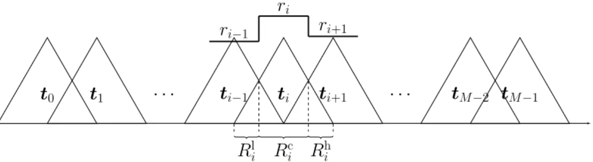
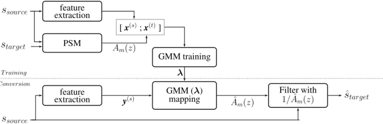
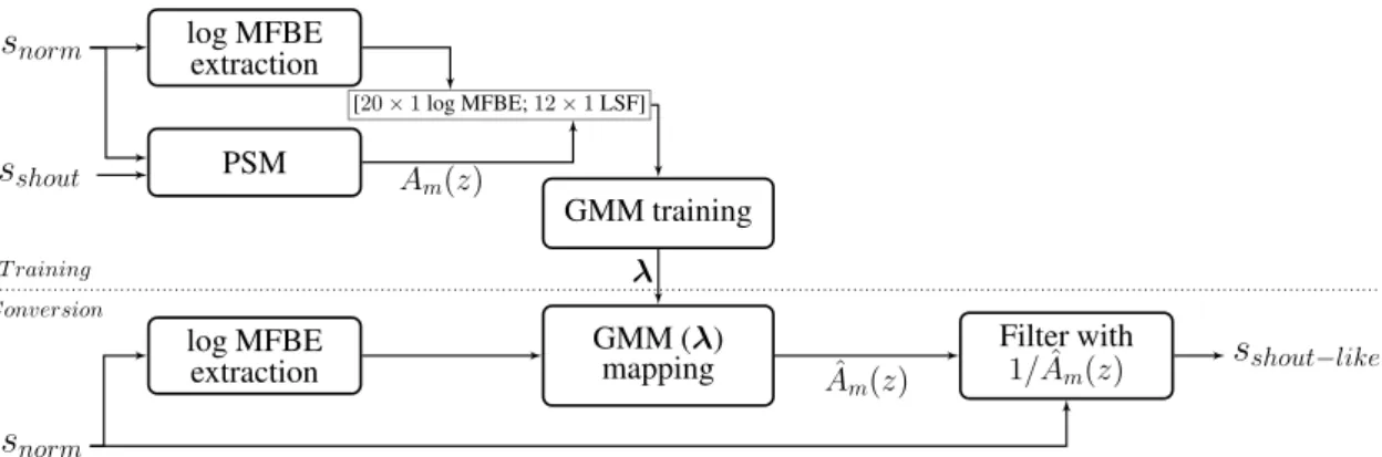
5 PSMGMM: A direct transformation SSC system 27 5.1 PSM . . . 27
5.2 PSMGMM algorithm . . . 31
6 Experimental work (topic I): Normal-to-shouted speech, PSMGMM-based SSC with application to speaker recognition under vocal eort mismatch 33 6.1 Data . . . 33
6.2.1 Speaker recognition system. . . 33
6.2.2 PSMGMM processing . . . 34
6.3 Evaluation . . . 35
6.4 Results . . . 37
7 A vocoder-based parametric SSC system 39 7.1 Vocoder framework . . . 42
7.1.1 Glottal vocoder framework . . . 42
7.1.2 The STRAIGHT vocoder framework . . . 46
7.2 Statistical mapping BGMMs . . . 49
8 Experimental work (topic II): Normal-to-Lombard-speech, vocoder-based parametric SSC using Bayesian GMMs 50 8.1 Data . . . 50
8.2 Experimental setup . . . 50
8.3 Evaluation . . . 51
8.4 Results . . . 52
9 Discussion and conclusions 55 9.1 Discussion of the denition of SSC . . . 55
9.2 Conversion of normal speech to high-vocal-eort speech . . . 55
9.3 SSC approaches: direct transformation vs. vocoder-based parametric 57 9.4 Discussion of mapping techniques . . . 59
List of abbreviations
ABE aperiodicity band energy AME attenuated main excitation
APLP adaptive pre-emphasis linear prediction ASR automatic speech recognition
BGMM Bayesian Gaussian mixture model
cycleGAN cycle-consistent generative adversarial network DFT discrete Fourier transform
DNN deep neural network DTW dynamic time warping EM expectation-maximization FFT fast Fourier transform
GD gender-dependent
GIF glottal inverse ltering GMM Gaussian mixture model
HMM Hidden Markov model
HNM harmonics plus noise model HNR harmonic-to-noise ratio
IAIF iterative adaptive inverse ltering
INCA Iterative combination of a Nearest Neighbor search step and a Con-version step Alignment method
JDE joint density estimation
KL Kullback-Leibler
LDA linear discriminant analysis LP linear prediction
LTI linear time invariant
MFBE Mel-scale lter bank energy MFCC Mel-frequency cepstral coecient MGC Mel-generalized cepstrum
MI mutual information
ML machine learning
MLE maximum likelihood estimation MMSE minimum mean square estimate MSE mean square error
NNLS non-negative least square
OLA overlap-add
PLDA probabilistic linear discriminant analysis PML pulse model in log-domain
PSM perceptual spectral matching PSOLA pitch-synchronous overlap-add QCP quasi-closed phase
RMS root-mean-square
SD speaker-dependent
SII speech intelligibility index SIIB speech intelligibility in bits SNR signal-to-noise ratio
SPL sound pressure level
SPSS statistical parametric speech synthesis SSC speaking style conversion
TTS text-to-speech
UBM universal background model
VC voice conversion
WER word error rate
List of symbols
List of Latin symbols
Am(z) transfer function of inverse lter of Hm(z)
AV T1(z) transfer function of inverse lter of HV T1(z)
D diagonal matrix with elements of |Hm( ˜Ω)|2 in its diagonal
E expansion matrix, to expand rˆ to full-length, NF F T-point power
spectrum
Etarget Mel-scale lter bank energy (MFBE) vector of target speech
f0 fundamental frequency
G(z) z-transform of glottal excitation airow Hm(z) transfer function of all-pole mapping lter
|Hm( ˜Ω)|2 matching lter power spectrum
hm(k) impulse response of Hm(z)
HV T1(z) transfer function of 1st-order all-pole lter of vocal tract model
i index for lters {ti} in lter bankT
Rc
i central region of lter ti
Rl
i lower region of lter ti
Ru
i upper region of lter ti
k speech time series index
L(z) transfer function of lip radiation eect
M number of lters in lter bank T
NF F T number of points (bins) in fast Fourier transform (FFT) used
p lter order of Hm(z)
r elementary power spectrum, which is a vector holding the values
of segments from piecewise constant power spectrum |Hm( ˜Ω)|2
ˆ
r estimate of r
ˆ ˆ
r full-length, NF F T-point power-spectrum of vector rˆ
S(z) z-transform of a speech frame
|Ssource( ˜Ω)|2 Mel-warped power spectrum of source speech
|Starget( ˜Ω)|2 Mel-warped power spectrum of target speech
ssource(k) source speech, that is, speech uttered in source speaking style
starget(k) target speech, that is, speech uttered in target speaking style
T uniform-scale triangular lter bank ti ith lter in lter bank T
V(z) transfer function of vocal tract
Dir(·) Dirichlet probability distribution
F dimension of feature vectors in X, and in Y
j mixture component index
J number of mixture components
Lj precision matrix of jth Student t's distribution component
m0 mean vector of the prior distribution (Gaussian-Wishart) over µj
mj mean vector of the variational posterior distribution
(Gaussian-Wishart) over µj, and also mean vector of jth
Student t's mixture component
N(·,·) Gaussian probability distribution
n observation index
N number of observations
p(·) probability distribution
q(·) variational (approximation) probability distribution
St(·,·,·) Student t's probability distribution
W(·,·) Wishart probability distribution
Wj scale matrix of the variational posterior distribution
(Gaussian-Wishart) overΣj
w weight vector of theJ Gaussian mixture components. wj weight ofjth Gaussian mixture component
X set of observed feature vectors, from source and target speech of one
frame (full training data)
x(s) observed feature vector of a source speech frame (training data)
x(t) observed feature vector of a target speech frame (training data)
Y set of observed and unobserved feature vectors, from source (observed)
and target (unobserved) speech of one frame
y(s) observed feature vector of a source speech frame
y(t) unobserved feature vector of a target speech frame
Z set of all latent variables (z) and parameters of
the Bayesian Gaussian mixture model (BGMM)
zn latent variable, 1-of-J binary vector associated to nth data point
znj latent variable vector element associated tonth data point.
List of Greek symbols
∆ rst-order delta coecients ∆∆ second-order delta coecients
ζ Mel-warping coecient
˜
Ω index of Mel-warpedFFT bins
α0 vector of pseudo observation counts of the prior distribution (Dirichlet)
overw
α vector of pseudo observation counts of the variational posterior
distribution (Dirichlet) over w, and weight vector of
αj weight of the jth Student t's mixture component
β0 scale of the prior distribution (Gaussian-Wishart) over µj
βj scale of the variational posterior distribution (Gaussian-Wishart) overµj
θ parameter set of a BGMM
λ parameter set of a Gaussian mixture model (GMM) Λj precision matrix of jth Gaussian component
µj mean vector ofjth Gaussian component
ν0 degrees of freedom of the prior distribution (Gaussian-Wishart) overΣj
νj degrees of freedom of the variational posterior distribution
(Gaussian-Wishart) overΣj
Σj covariance matrix of jth Gaussian component
Comments on notation:
The symbols on the thesis marked with a hat are an estimate of the given variable. For example, yˆ(t) is an estimate of y(t).
Humans can vary their speaking style, and indeed they change it constantly in their daily interactions. Speaking style varies depending on many factors, such as the context of the situation, the state of the speaker, or the personal and social relationship of the speaker with the other interlocutors of the conversation. Thus, given the ubiquity of speaking style in natural speech, it is important that speech technology adapts to it with the objective of obtaining more realistic results. One way to achieve this is by including speaking style conversion (SSC) as a part of the steps performed in the current speech technology. SSC performs an acoustic-to-acoustic conversion of the original speaking style of a speech utterance (denoted henceforth as the source speaking style) to another speaking style of our choice (denoted henceforth as the target speaking style). Then, for example, whispered speech could be converted to shouted speech, or normal (neutral) speech could be converted to sad speech (that is, speech uttered in sad emotion).
If we pay attention to the dierent aspects in which someone's speaking style may change, we can notice that the style can vary for example in terms of emotion and/or of vocal eort. When performing SSC that is focused on emotion, often denoted plainly as emotion conversion (e.g., [1, 2, 3, 4]), the focus in conversion is mainly in paralinguistic attributes of speech, such as prosody and intonation. In case ofSSCfor vocal eort, speech attributes such as energy/intensity, loudness and pitch of the signal become more important for an optimal conversion. Nevertheless, these two aspects of conversion (emotion and vocal eort) are not entirely sepa-rate, and become sometimes completely intermingled; for example, in case of angry speech [5]. Given all the aforementioned changes in speech attributes for dierent speaking styles, the main challenge of SSC tasks is to achieve speech conversion by transforming (some of) those attributes while at the same time retaining the voice (that is, the speaker identity) and the linguistic content of the utterance. In addi-tion, it is essential that the SSC system does not sacrice speech quality to achieve converted samples that show a clear target speaking style. That is, rather than hav-ing a compromise between speech quality and degree of conversion, it is desirable to have a SSC system that achieves to have both.
SSC applications include those where the end user is a human listener and those where the end user is a machine learning (ML) system. In the case of vocal-eort-focusedSSC, applications intended for human listeners include making the converted speech signal more intelligible. For example, soft speech (such as whispered speech) could be converted to normal speech to make it more understandable, or normal speech could be converted to Lombard speech [6] in order to make it more intelligible when listened to in noisy situations. In addition, normal speech could be converted to so-called clear speech [7, 8], which facilitates comprehension for the listener. These applications are most benecial for people with hearing impairments or for people who have diculties in understanding speech produced using normal speaking style. Another potential application of vocal-eort-focused SSC (and SSC in general) for human listeners, could be the customization of speech according to the preferences of the end user. For example,text-to-speech (TTS)concatenative synthesis systems'
output speech could become more exible and personalizable in accordance to the user needs, without the need of a bigger data set. This could be achieved by applying SSCto the synthesized samples [9, 10]. On the other hand, someSSCsolutions could be employed in a parametric speech synthesis system, by deploying rules based on SSC to perform speaking style modications [11].
Vocal-eort-focused SSC can prove to be useful also for speech computer-based tasks, as we will see next. Humans have the innate skill of being able to cope with variation in speech (for example, changes in accent, vocal eort, or voice mimicry) during everyday tasks, such as speech or speaker recognition. In contrast, variations in speech recordings pose a challenge for computer-based systems. Typically, studies comparing the performance of humans and machines at speech-related tasks have shown that humans usually outperform machines [12, 13, 14]. Nevertheless, the advances in speech technology over the years have decreased the performance gap between machines and humans; in some cases, machines managed to equal or even slightly surpass humans. The latter has been shown for example in some studies on speaker recognition or verication for voice mimicry or disguise [15, 16, 17] and also in some studies on speech recognition [18]. In case of vocal eort variations, a common case of mismatch occurs for speaker recognition or verication tasks in forensic cases: the system is usually trained on normal speech, while the speech samples under evaluation are sometimes uttered by a speaker that is in an agitated or stressed state. Such mismatch harms the performance of the system [19, 20]. By decreasing the mismatch, the recognition performance could improve [21, 22, 23]. Thus, vocal-eort-focused SSC can be applied in such cases. We should note that SSC applications oriented to ML systems dier from those oriented to human listeners in that the converted speech samples do not require to retain the subjective speech quality of the original signal.
SSC methods use mainly two approaches: a vocoder-based parametric approach, and a direct transformation approach. The vocoder-based parametric approach em-ploys a vocoder to extract features from a speech signal, a subset of those features are then modied, and nally the vocoder, having as input all features (modied and unmodied), synthesize the converted speech signal. In contrast, the direct trans-formation method involves converting directly the source speech signal to target speech, by applying operations (such as ltering) directly onto the speech signal, or onto the speech signal once transformed to another domain (e.g. spectral domain). The transformation of the features can be automatic, using ML-based mapping techniques. Some mapping methods employed for SSC require having parallel data for tting their models. Obtaining parallel data for speaking styles is quite costly in general and thus this kind of databases are scarce. Therefore, some mapping techniques have been used in SSC specically to cope with the problem of needing parallel data for mapping.
SSC has relation with other areas in the speech technology eld, such as voice conversion (VC)[24],statistical parametric speech synthesis (SPSS)[25] and speech enhancement in speech transmission [26]. Nevertheless, SSC can be understood as a research area on its own due to its dierences with the other aforementioned areas. For example, there is no linguistic-to-acoustic conversion as in SPSS. On the
other hand, SSC is not constricted by strict latency constraints which are present in enhancement applications in speech transmission technology.
1.1 Thesis scope
This thesis focuses on speaking styles that dier in terms of vocal eort. Specically, the focus is on conversion from normal speaking style to a speaking style uttered in high vocal eort. Based on this aim, we studied two dierent topics on SSC in this thesis: the rst topic dealt with normal-to-shouted speech conversion and the second topic dealt with normal-to-Lombard conversion. In this thesis, we present experimental work from these two topics based on the following peer-reviewed arti-cles:
[22] A. Ramírez López, R. Saeidi, L. Juvela, and P. Alku, Normal-to-shouted speech spectral mapping for speaker recognition under vocal eort mismatch. in 2017 IEEE International Conference on Acoustics, Speech and Signal Pro-cessing (ICASSP), 2017, pp. 49404944.
[27] A. Ramírez López, S. Seshadri, L. Juvela, O. Räsänen, and P. Alku, Speaking style conversion from normal to Lombard speech using a glottal vocoder and Bayesian GMMs. in Interspeech, 2017, pp. 13631367.
The SSCsystem that we proposed in the rst topic used a direct transformation approach, that we denoted asperceptual spectral matching (PSM)-Gaussian mixture model (GMM) (see Sections 5 and 6). This system had direct application in a speaker recognition framework in which there is mismatch of vocal eort between the enrollment and test utterances. In the work we have done on this rst topic, the main research question under study was to test how eective SSC would be when used together with a computer-based speech system (in this case, a speaker recognition system), rather than having as end-user a human listener. In order to answer this research question, we evaluated the speaker recognition system performance in two dierent cases: with and without employingSSC. A side research question consisted of studying if theSSCsystem was able to convert speech without degrading speaker identity. The SSC system that we proposed for this topic has the novelty of being, to the best of our knowledge, the only SSC work proposed for direct application in speaker recognition with vocal eort mismatch.
The SSC method that we proposed for the second topic, was a vocoder-based parametricSSCsystem (see Sections7and8). We evaluated this method in terms of speech quality using the converted speech samples in subjective listening tests. With this evaluation, we mainly focused on studying if it is possible to achieve adequate conversion of speech (in the specic case of normal-to-high-vocal-eort conversion) without producing degradation in quality. A secondary research question in this topic was to evaluate if the newer version of a glottal vocoder proposed in [28] that we employed would provide better speech quality in the converted samples than the widely used STRAIGHT vocoder. In addition, a minor research question was to test if the mapping system we selected (Bayesian Gaussian mixture models (BGMMs))
would function adequately and cope with the scarcity of the training data. Finally, we should note that the work we have performed on this topic has the novelty of using BGMM-based mapping for the rst time in a SSC study.
1.2 Thesis structure
The present thesis consists of a theoretical background and experimental work in SSC of normal speech to high vocal eort speech. We present the theoretical back-ground in Sections2-4. Section2covers details about the speech production process and developed theory for modelling it, which is a foundation to the vocoders em-ployed in the second topic of this thesis. We present also details of the vocoders used. In addition, given that we are focusing in this thesis on conversion of normal speech to high vocal eort speech, this section also describes dierences in speech attributes between these styles of speech. Section 3 introduces a brief overview of the mapping techniques employed forSSC, and it goes more in depth onto the map-ping techniques that we employed in the experimental works included in this thesis. Finally, Section4 presents a review of high-vocal-eort-focused SSC.
We present the experimental work for each topic, along with theory of the SSC methods employed in each topic, in Sections 5-8. We organized the sections as follows. First, Section5 presents the theory of the rst topic: we proposed a direct-transformation-basedSSC system forSSCof normal speech to shouted speech, with a speaker recognition application under vocal eort mismatch. This study corre-sponds to work published in [22]. We then present the experimental work on this topic in Section 6. Second, Section 7 introduces the theory of the second topic: a vocoder-based parametric SSC system we proposed, to transform normal speech to Lombard speech. The work from this second topic has been previously published in [27]. We present the experimental work of the second topic in Section 8. Finally, Section9 presents overall discussion and conclusions from this thesis.
2 Speech production and its modeling
2.1 The speech production mechanism
If we think of the mechanism of human speech production from a signal point of view, we can consider speech production as a two-step process. In the rst step, we generate airow by exhaling air from our lungs through the trachea, and then the airow passes through the vocal folds at the larynx. If our vocal folds are open when the airow passes through, an excitation signal is created corresponding to unvoiced speech. In the case of voiced speech, the vocal folds are tense, vibrate and collide, such that the airow signal is modulated. As a result, an excitation signal, in the form of quasi-periodic pulses, is generated. This voiced excitation signal is frequently referred to as glottal ow1 or voice source. The rate at which
the vocal folds vibrate indicate the value off0 (the fundamental frequency), which is
the pulse frequency of the glottal ow signal. Glottal ow signal thus generates the harmonic spectral structure of speech given by f0 and its harmonics. In contrast,
the unvoiced excitation lacks the harmonic structure, because the vocal folds do not vibrate periodically.
In the second step, the excitation signal passes through our vocal tract and is radiated via our mouth and nostrils. The vocal tract consists of the following articu-lators: pharynx, oral and nasal cavities. The vocal tract lters the excitation signal, since the vocal tract articulators act as cavity resonators and create resonances (also called formants) that shape the excitation signal in the spectral domain. We can modify at will the resonances by changing the position or shape of our vocal tract articulators. Thus we humans are capable of creating speech signals of dierent for-mant values which is very important for recognition of phonemes. The vocal tract dimensions and shape vary across gender, age, and even across individuals [29, 30]. In consequence, even if a group of people would utter speech sounds representing the same phoneme, the produced signals would show dierences in spectral content and the formants of the signals would also not be exactly same. In the case of unvoiced speech, the airow is constricted partially (or totally for a short instant for the so-called plosives) at some point of the vocal tract. As result, unvoiced speech shows a noise-like waveform (or impulse-like for plosives). Figure 1 presents a simplied sketch of the human speech production mechanism.
2.2 Sourcelter modeling
The two-step notion of speech production, covered in Section2.1, is the foundation of sourcelter theory [29], widely used in speech modeling. The speech production mechanism is modeled as an excitation signal (the source) that excites the vocal tract (the lter) and this one in turn shapes the spectrum of the signal. Figure 2 presents a block diagram of speech production modeling with sourcelter theory.
1In acoustics, the correct term for the the voiced excitation signal is the glottal volume velocity waveform, but it is commonly just referred as the glottal ow. The `glottal' naming references the V-shaped opening between the vocal folds, denoted as glottis.
Nostrils
Lips
Nasal cavity
Oral cavity
Pharynx
Larynx opening into pharynxVocal folds
Larynx
Trachea
Lungs
Figure 1: Speech production mechanism.
filter source output Nasal cavities Mouth cavities Pharynx cavities Vocal folds airf low (f rom lungs) nasal sound pressure wave oral sound pressure wave
Figure 2: Schema of sourcelter model of speech production, adapted from [29, 31]. In the case of voiced speech, the excitation signal is the glottal ow, which is the result of vocal folds vibrating when airow passes through them. Thus, the glottal ow spectrum presents harmonics and the magnitude spectrum decreases with the frequency, at a rate of 12dB per octave [32]. In the case of unvoiced speech, we can assume the excitation signal to be white noise, since for unvoiced speech the airow is constricted somewhere in the vocal tract which results in a noise-like signal. The
vocal tract (seen as an acoustic tube) modulates the source signal and generates formants that amplify the spectrum magnitude of the source signal at the formant's frequency and its surrounding2. After passing through the vocal tract, the signal
radiates through the mouth and nose as a sound pressure wave and we are able to hear it. When the conversion from airow to pressure wave occurs, a lip radiation eect is observed, resulting from the change in acoustic impedance between the lips and the surrounding air. We can approximate the lip radiation eect by the rst derivative of the airow, so it behaves like a high-pass lter and the spectrum magnitude increases at a rate of 6dB per octave [32]. Thus, in a digital system we can approximate the lip radiation eect to a rst-order dierentiator, which in the
z domain is represented with the following transfer function:
L(z) = 1−γz−1, (1)
whereγ is a constant value. Usuallyγ ≤1, to ensure stability when the lip radiation
eect needs to be cancelled by inversion.
The sourcelter model assumes that the two components that conform speech, source and lter, are independent of each other and thus they can be computed independently. In addition, the model assumes the lter to belinear time invariant (LTI). Given these assumptions, speech can be represented using the sourcelter model, in the z domain, as [29, 33]:
S(z) =G(z)V(z)L(z), (2)
where G(z) is z-transform of the glottal source signal, V(z) is the transfer function of the vocal tract, andL(z)is the transfer function of the lip radiation (Eq.1). The lip radiation eect is frequently combined with the glottal source component, and then speech can be expressed as:
S(z) = G0(z)V(z), (3)
where
G0(z) = G(z)L(z). (4)
The sourcelter model is a simplication of the actual speech production mecha-nism, and therefore has some drawbacks. The main aw comes from the assumption of independence between the source and lter elements of the model, while in real-ity there is interaction eects between these two [34, 35]. Another aw involves the assumption of having a LTI lter: while the model is accurate enough for sounds that vary slowly (like voiced speech), there are other sounds (for example, plosive consonants like /p/ or /k/) which are more rapidly changing. In such cases, the model fails at representing speech accurately. In addition, vocal tract is commonly represented with an all-pole lter (which is frequently computed using linear pre-diction (LP) [36]). Thus, sounds with anti-resonances (like nasal sounds), which require having zeros in the lter, will be poorly modeled. Nevertheless, we can solve 2In the case of nasal sounds, anti-resonances can also be created, which attenuate the spectrum magnitude.
this issue by adding extra poles to the lter [37]. We should also note that given the coupling eects between lter and source that the model neglects, the all-pole lter is most likely modeling not only the vocal tract but also some contributions of the source and lip radiation eect. The aforementioned aws limit the accuracy of the sourcelter model. The coupling eects between source and lter may aect specially the performance of speech applications focusing on generating speech or modifying it, since for those applications the naturalness in speech is a key matter. In other applications, such as speech coding, sourcelter modeling proves to be good enough.
2.3 Sourcelter vocoders
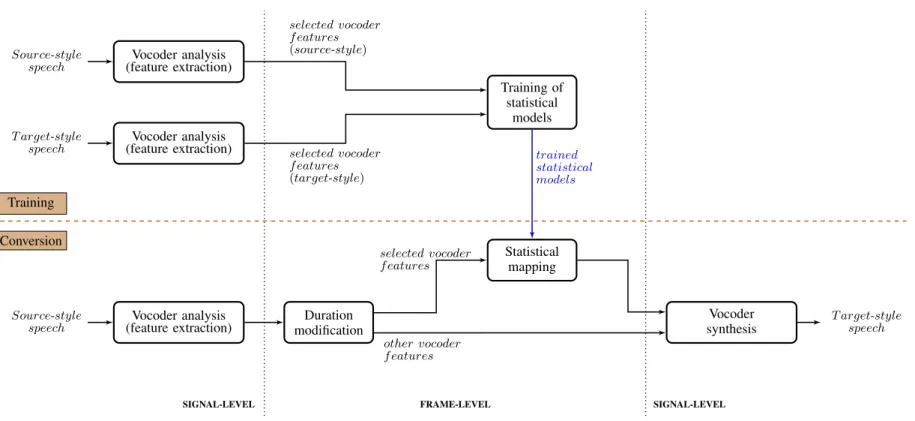
SPSS tasks have at their core a vocoding system: 1) A vocoder is used during the training stage, to extract features that represent the speech signal. The features are then used to train statistical generative models. These models are indexed with a linguistic specication, which gives textual context information, and it is stored for later retrieval. 2) A vocoder is also used in the synthesis stage. In this phase, linguistic specications extracted from text are used as input to retrieve the trained statistical models, which in turn estimate the speech features. Finally, these features are used as input to the vocoder, to reconstruct the speech signal [38, 39]. As mentioned in Section 1, while speech technology applications such asSPSS,VC and SSC have dierent goals, there is some relation between them. In VC andSSC a vocoder is often employed also as part of the system.
Most commonly, vocoders are based on the sourcelter model (e.g. STRAIGHT [40, 41], WORLD [42], GlottHMM [43], GlottDNN [44], pulse model in log-domain (PML) [45] and GSS [46]). There are also vocoders employing other models: for example, using the harmonic (or sinusoidal) model, which represents speech as a sum of sinusoids [47] (e.g. Ahocoder [48] and HMPD [49]) or the dynamic sinusoidal model, in which a time-varying term is added to the standard sinusoidal model for amplitude renement [50] (e.g. PDM [51, 50]).
In the experimental work from the second topic included in this thesis, we em-ployed two sourcelter vocoders: a glottal vocoder and STRAIGHT. Thus, these two vocoders are explained in detail next.
2.3.1 The glottal vocoder
Glottal vocoders are based on the sourcelter parametric model [29], such that speech can be represented as a convolution of the vocal tract lter and glottal ow excitation (the latter one includes also the lip radiation eect) [29, 52]. For the second topic of this thesis, we employed a glottal vocoder that is a variant imple-mentation of the glottal vocoder introduced in [28]. This vocoder was created at rst forSPSS applications [25]. It employs for voiced frames aglottal inverse lter-ing (GIF) method based on the sourcelter model to split the speech signal into a vocal tract lter and glottal ow excitation. GIF methods are able to estimate the glottal ow of the speech signal by cancelling out the eect of the vocal tract and
lip radiation. When the sourcelter model is assumed for speech production (see Eqs. 2-3), GIF estimates the glottal ow in a voiced segment as:
G(z) = S(z)
V(z)L(z). (5) where G(z) is the z-transform of the glottal ow, S(z) is the z-transform of the speech signal, V(z) is the transfer function of the vocal tract and L(z) the transfer function of the lip radiation eect. As seen in Eq. 1, we can express lip radiation as a rst-order dierentiator; thus, the main task is to estimate the vocal tract element accurately. A frequent issue when estimating the vocal tract is harmonic bias: formants are aected by this bias and their estimates tend to shift towards harmonics generated by the voice source. This is specially true for high-pitched signals (such as those uttered by female speakers), which show sparse, high-energy harmonics.
The glottal vocoder that we employed here uses specically the quasi-closed phase (QCP) GIF method [53], which is based on closed phase analysis. In this approach, the vocal tract spectrum is estimated during the closed phase of the glottal excitation, i.e. when the glottis is closed. At this time, the voice source's inuence on the vocal tract's spectrum is minimal. QCP uses weighted linear prediction (WLP) [54] and the attenuated main excitation (AME)weight function that minimizes the biasing eect from the harmonics of the glottal ow signal when estimating the vocal tract's spectrum [53]. In the case of unvoiced segments, the vocoder uses a random noise excitation signal and conventionalLPfor the vocal tract. In addition, this vocoder uses a deep neural network (DNN) model to generate the glottal ow pulses [55], which are employed in the synthesis step. Lastly, to parametrize speech, the glottal vocoder extracts during analysis the following features: 1) log-energy, 2) harmonic-to-noise ratio (HNR), 3)f0, 4) vocal tractline spectral frequencies (LSFs),
denoted here as LSFV T, and 5) glottal source LSFs, denoted as LSFglott.
2.3.2 The STRAIGHT vocoder
STRAIGHT is a known vocoder, often used in SPSS, which also uses as foundation the sourcelter model [29]. The STRAIGHT vocoder estimates during analysis a cepstrum-based spectral envelope for the vocal tract using a pitch-adaptive time-frequency smoothing method. This method also aims to minimize the biasing eect generated by the harmonic peaks to the vocal tract spectrum [40, 41]. In addition, STRAIGHT employs a mixed excitation signal during synthesis. This kind of signal involves: 1) a periodic train of pulses, mixed with 2) an aperiodic noise signal, which is added to several frequency bands based on some aperiodicity weights. The mixed excitation signal is used for voiced segments, while a white Gaussian noise excitation signal is used for unvoiced segments. Finally, the features that this vocoder extracts during the analysis stage are: 1) theaperiodicity band energies (ABEs), to represent the aperiodicity spectrum, 2)f0, and 3) the spectral envelope, which is represented
2.4 High vocal eort speech
When the focus is on speech uttered using dierent vocal eorts, we can consider that the dierent vocal eort modes dene a kind of continuum, from low to high vocal eort. There are many examples of vocal eort modes on the continuum such as whispered speech, soft speech, normal speech, loud speech, Lombard speech, and shouted speech. However, we should note that these examples of vocal eort modes are not completely separate and acoustical speech features belonging to the dierent modes on the continuum typically overlap. In this thesis, our focus is on speaking styles of high vocal eort, which are compared to the speaking style used in production of speech of normal vocal eort.
For ecientSSC, the system should use speech attributes that most prominently dier between the source speaking style and the target speaking style. In the ex-perimental work of this thesis, the source speaking style was in all cases normal speech, while the target speaking style was Lombard speech in the second topic and shouted speech in the rst topic. Next, we present the speech attributes of both target speaking styles (Lombard speech and shouted speech), and compare them to those of the source speaking style (normal speech).
2.4.1 Lombard speech
There are certain speech production mechanisms that humans employ to enhance the intelligibility of their speech. For example, humans increase their vocal eort (and in turn they increase their loudness) to be heard more easily. The increase in vocal eort is an involuntary reex, known as the Lombard eect [6, 56, 57], that humans adopt when they are placed in adverse acoustic environments (i.e. noisy conditions) [58].
The dierence in loudness between normal and Lombard speech is the most evident speech attribute that changes between these two styles. However, there are also other changes aecting the speech. One is the dierence in duration between normal and Lombard speech: there is an increase in duration for Lombard speech in comparison to its normal speech counterpart [58, 59, 60]. Another speech attribute dierence isf0, which also increases for Lombard speech [58, 59, 61]. In addition, the
spectral content of the speech signal varies from one style to the other. Specically, in Lombard speech, the energy of higher frequencies is typically larger compared to normal speech. In other words, the spectrum of Lombard speech shows a atter tilt compared to normal speech [60, 61]. Within all these attributes, spectral tilt has been shown to inuence most for the intelligibility enhancement provided by Lombard speech [61]. Finally, we should note that the type of noise that triggers the Lombard eect [60] and the gender of the speaker [62] aect the quantity and manner in which these speech attributes change.
2.4.2 Shouted speech
Humans utter in shouted speaking style when for example a person tries to commu-nicate with another person over a distance [63], or when the speaker is in an agitated
or stressful state [64]. We can encounter the latter situation often in forensic cases [65]. While shouted speech is at the end of the vocal eort continuum, and thus shows typically a highersound pressure level (SPL)value than Lombard speech, the use of shouted speech is less intelligible compared to Lombard speech, or normal speech. The reason for this is the reduced use of articulation during the production of shouted speech [66, 67].
Apart from the increase in SPL [20], also other speech attributes change for shouted speech in comparison to normal speech. For example,f0increases in shouted
speech [68, 69, 65] as well as the rst formant (f1). [70, 69, 65]. Regarding the
spectral distribution, the spectral tilt in shouted speech decreases in comparison to normal speech [20, 71, 69]. On the other hand, the duration of utterances produced using shouting increases in comparison to the same utterances uttered in normal speaking style [68, 20]. This increase in duration is due to an increase in word duration, rather than in silence duration (as it occurs in whispered or soft speech) [20].
3 Mapping techniques
Several approaches exist for mapping speech features of the source speaking style to speech features of the target speaking style. SomeSSC methods employ signal pro-cessing methods only in their approach, while other methods employ a combination of signal processing and ML techniques in the conversion. The SSC methods that only employ signal processing can be understood as deterministic approaches, given that in that case we are applying a xed solution to all the speech input signals. Among high-vocal-eort-focusedSSCworks, [11, 72, 10, 73] employ only signal pro-cessing. Out of these, [10] studies a scenario in which parallel data of the source and target speech is required, since vocal eort modication is based on transfer-ring features of target speech to source speech. While deterministic approaches, like the aforementioned ones, tend to be computationally cheaper, data-drivenSSC approaches (that is, approaches that include ML along signal processing) are usu-ally more eective due to their exibility: the solution proposed is adaptive to the given data, rather than xed. The adaptation is based on the trained model that the data-driven approach employs. Thus, data-driven mapping techniques require training data of the source and target signals to t in the model.
In the case of speech applications, some mapping techniques require to have a data set of parallel training speech samples. That is, pairs of speech samples that have the same attributes (such as text, voice, or speaking style), except for the attribute that is being mapped: one sample out of the pair will have the to-be-mapped attribute from source speech, while the other sample will have that attribute from target speech. ForSSC, the training data set consists of pairs of speech samples for the source and target that has the same voice identity (speaker) and linguistic content (that is, the same text), but one sample is uttered by the speaker in the source speaking style, and the other samples is uttered in the target speaking style. Other mapping techniques can be trained with non-parallel data. This means that the speech samples from source and target speech do not need to correspond to the same linguistic contents. For this reason, parallel data is also referred to as text-dependent data, while non-parallel data is referred to as text-intext-dependent data. Based on the type of data required in training, we can group data-driven mapping techniques into two main categories: parallel mapping and non-parallel mapping.
3.1 Data-driven, parallel mapping
Many data-driven mapping approaches forSSChave been adopted from theVCeld, in which more research has been conducted. In the case of parallel-based approaches, GMMshave been, for example, used for mapping inSSC, and were rstly proposed inVC[74, 75]. In high-vocal-eort-focusedSSCstudies,GMMshave been applied in [9, 22]. GMMs were also employed in [76], and were compared against feed-forward DNNs, andBGMMs; the latter ones are an extension ofGMMs, and are more robust to scarce training data than GMMs. BGMMs have also been used earlier in [27]. Robust mapping techniques are key in case ofSSC, since collecting data in dierent speaking styles is very costly; this is specially true for parallel data.
In a parallel data set, often the pairs of source and target speech signals do not match in duration. Thus, prior to using the parallel data set in mapping, its source-target speech pairs need to be time aligned. A common approach for alignment at frame-level is dynamic time warping (DTW) [77, 78, 79, 74]. Other approaches are those that performHidden Markov model (HMM)-based phonetic aligments [80, 81] or sentence HMM-based alignments [82]. The performance of the alignment task, to pair the source and target frames, also inuences the outcome of the conversion tasks. This topic is not covered in the present thesis, but it has been studied for example in [83].
In this thesis, we present two topics that include data-drivenSSCsystems. These topics involve mapping using GMMs in one case (rst topic) [22], and BGMMs in the other (second topic) [27]. Thus, next we describe in detail these two kinds of statistical models.
3.1.1 GMM mapping
GMMis a probabilistic model widely used to represent continuous features in speech technology methods such as inautomatic speech recognition (ASR)[84] or VC[74]. GMMsare continuous, parametric density functions that consist of a weighted sum of Gaussian distributions (denoted as the mixture components of theGMM). When we employ a GMM to model the observed data X, each observation (Xn, where
n= 1,2, . . . , N, andN is the total number of observations available) we are assuming
each observation to come from one of the Gaussian components of theGMM, though it is unknown to us from which specic component. In other words, we are assuming that X presents a hidden cluster-like structure and the GMM's components model
the underlying, latent classes in the data (with each of these classes assumed to follow a Gaussian distribution) [85]. Thus, in this model, each observation sample (Xn)
has associated a latent variable (zn) that indicates from which mixture component
the data point originates. Latent variablezn = [zn1, zn2,· · · , znJ]is a binary vector,
in which all elements are random binary variables (that is, znj ∈ {0,1}), and J is
the number of Gaussian components of the model. Of all the vector elements in zn,
only one is 1, for exampleznj0=1, while the rest of vector elements inzn are 0. This
indicates that the corresponding data sampleXn belongs to thej0th component of
the GMM. Thus, theJ elements of vectorzn always add up to 1:
PJ
j=1znj = 1.
We can express the likelihood of X as:
p(X|λ) =
J
X
j=1
p(zj = 1|λ)p(X|zj = 1,λ), (6)
where λ are the GMM parameters, p(zj = 1|λ) is the prior probability of the jth
mixture component, and p(X|zj = 1,λ) is the jth component density function.
Given that: 1) p(zj) is often denoted as wj, that is:
and 2) the probability density functions of each GMM component is a Gaussian distribution:
p(X|zj = 1,λ) = p(X|λj) = N(µj,Σj); (8)
then, using Eqs.7-8, we can express the likelihood from Eq.6 as:
p(X|λ) = J X j=1 wjN(X|µj,Σj), J X j=1 wj = 1 (9)
where wj =p(j|λ) is the mixture weight of the jth component, (as mentioned, the
prior probability of jth mixture component); and µj and Σj are the mean vector
and covariance matrix, respectively, of the jth component. In addition, J is the
number of mixture components. Thus, the parameters of the model to estimate are
λ = {µ,Σ,w}, where µ = {µj}, Σ = {Σj}, and w = {wj}, for j = 1,2, . . . , J.
The estimation of the GMM parameters is typically computed by using maximum likelihood estimation (MLE). Figure 3 shows a graphical model of a GMM.
X
nz
nN
µ
jw
jΣ
jJ
Figure 3: Graphical model of aGMM, adapted from [86]. Nodes represent variables; the node marked in pink corresponds to a observed variable. In addition, red notches indicate point estimates of parameters (that is, xed values), and arrows represent conditional dependencies. Finally, the plates indicate repetition over the respective index. Thus, on one hand there is a set ofN i.i.d. observed data points{Xn}, with
corresponding latent points{zn}, with n= 1,2, . . . , N; and on the other hand there
are the parameters {wj}, {µj}, and {Σj}, of mixture components j = 1,2, . . . , J.
GMMs have been used rstly in the context of VC (e.g. [75]), and later in SSC (e.g. [22]), because of the cababilities of GMMsto model the dependencies between
the feature vectors of a source speech frame (x(s)) and the feature vectors of a target
speech frame (x(t)). The joint density estimation (JDE) approach [75], often used
with GMMs, implies that concatenated feature vectors X = [(x(s))|,(x(t))|]| are employed for training theGMM (that is, estimating the GMM parameters λ) that
models the joint density function of source and target features, p(X|λ). As we can appreciate in Eq.9, this density is the likelihood ofX, and we can use it afterwards
for mapping feature vectors of source speech to those of target speech. In this case, we can rewrite Eq.9 as follows:
p(X|λ) = J X j=1 wjN "x(s) x(t) # " µ(js) µ(jt) # " Σ(js,s) Σ(js,t) Σ(jt,s) Σ(jt,t) # , J X j=1 wj = 1 (10) where µ= µ(js) µ(jt) and Σ= Σ(js,s) Σ(js,t) Σ(jt,s) Σ(jt,t) .
We can compute maximum-likelihood estimates of the model parametersλusing
the expectation-maximization (EM) algorithm [87]. This is an iterative algorithm, which (after an initial estimate of the model parameters) alternates between two steps: 1) Expectation step: computing the expected values of zn, given the current
estimate of model parameters λ. The expectations of {zn} are denoted as
respon-sibilities, i.e. rn =E(zn). 2) Maximization step: updating the model parameters λ
with their best maximum-likelihood-based estimates, while keeping xed the values of the current responsibilities. The iteration between these two steps continues until the algorithm reaches convergence [87]. Some of the disadvantages ofEM is that it is very sensitive to the initialization of the parameters, and it requires to determine the number of GMM components (clusters) beforehand. We can interpret EM as a soft version of the k-means algorithm. Apart from the disadvantages coming from
the EM algorithm, using GMMs also has some downsides. The main disadvantage of GMMs is that given that the parameters are xed, there is not indication of the uncertainty of their estimated values.
After we have trained the GMM with the EM algorithm, we can predict the target feature yˆ(t) as the mean square error (MSE)estimate of y(t) given data y(s):
ˆ y(t) = J X j=1 p(j|y(s),λ) µ(jt)+Bj(y(s)−µ (s) j ) , (11)
where µ(jt) and µj(s) are the mean vectors of the jth component for x(t) and x(s),
respectively. We can compute the posterior component probabilities p(j|y(s),λ)
from prior component probabilitieswj and likelihoods N(y(s)|µ
(s) j ,Σ (s,s) j ) as p(j|y(s),λ) = wjN(y (s)|µ(s) j ,Σ (s,s) j ) PJ j0=1wj0N(y(s)|µ (s) j0 ,Σ (s,s) j0 ) , (12)
and we obtain the linear transformations Bj as
Bj = (Σ
(t,s)
j )
−1Σ(s,s)
where Σ(jt,s) and Σj(s,s) are correlation matrices concerning x(t) and x(s).
3.1.2 BGMM mapping
BGMMs are an extension of GMMs that give better generalization performance, since BGMMs adapt their complexity depending on the data at hand. That is, rather than having a pre-xed number of components as in GMMs, the number of components are stochastically selected as a function of the data structure. Another advantage of using a Bayesian framework is that it is less sensitive to parameter initialization.
In conventional GMMs, the parameters or the model are deterministic, and we employ a maximum likelihood approach (MLE) to obtain point estimates of the parameters (see Section 3.1.1). The Bayesian framework includes prior probability distributions for theBGMM parameters, such that the parameters behave stochas-tically. In this approach, the goal is to infer the posterior distribution of the pa-rameters. Therefore, the Bayesian approach involves prior, likelihood and posterior functions, since the joint prior distribution is updated with data evidence to obtain the posterior distribution, via the Bayes' rule:
posterior= prior×likelihood
evidence (14)
In this framework, estimating the predicted distribution of target speech features (y(t)) requires marginalizing out the model parameters, since the parameters are
modeled as random variables. Figure 4 shows a graphic model representation of a BGMM.
In the context of SSC, to estimate the posterior distribution parameters, we construct training data vectorsXby concatenating a feature vector of source speech
(xs)) and a feature vector of target speech (x(t)): X = [(x(s))|,(x(t))|]|. Each sample (Xn) has associated a latent observation (zn), which is a 1-of-J binary
vector with elements znj for j = 1, . . . , J. The number of Gaussian components
is J, and znj = 1 if the observation belongs to the GMM's jth component, and 0
otherwise. That is, there is an underlying cluster-like structure in the data. We can represent the conditional distribution of latent variables z given weight coecients w as: p(z|w) = J Y j=1 wzj j , (15)
and the conditional distribution of the observed data, given the latent variables and model parameters, is of the form:
p(X|z,w,µ,Λ) =
J
Y
j=1
N(X|µj,Σj)zj. (16)
X
nz
nN
µ
jw
jΛ
jJ
α
0W
0ν
0m
0β
0Figure 4: Graphical model of a BGMM, adapted from [86]. The nodes represent variables (and the node marked in pink is an observed variable). The red notches in-dicate point estimates of the hyper-parameters, and the arrows represent conditional dependencies. In addition, the two plates indicate repetition over the corresponding index, such that there is a set of N i.i.d. observed data points {Xn}, with
corre-sponding latent points {zn}, with n= 1,2, . . . , N, and parameters {wj},{µj}, and
{Λj} of mixture components j = 1,2, . . . , J. express it as: p(X|θ) = J X j=1 wjN "x(s) x(t) # " µ(js) µ(jt) # " Λ(js,s) Λ(js,t) Λ(jt,s) Λ(jt,t) # , J X j=1 wj = 1, (17)
where nowθ ={µ,Λ,w} represents the BGMM parameters3, and µ={µj}, Λ=
{Λj}, and w ={wj}, for j = 1,2, . . . , J. J is the number of mixture components,
wj = p(j|θ) is the prior probability of the jth component; and µj and Λj are the
3In this thesis, we representBGMMparameters with a dierent variable than the one used for
GMMparameters, to emphasize the dierence in nature between these two cases: GMMparameters (λ) are xed whileBGMMparameters (θ) are random variables.
mean vector and precision matrix4 of eachjth component, respectively [74, 75].
Next, we need to select the prior probabilities of the model parameters, θ. For
that, we have to take into account that the analysis is largely simplied if we choose conjugate priors. Thus, we select for mean and precision of each Gaussian compo-nent, a Normal-Wishart distribution:
p(µj,Λj) = p(µj|Λj)p(Λj) = N(µj|m0,(β0Λj)−1)W(Λj|W0, ν0), (18)
where m0 denes the center, constant β0 indicates how far the mean is on average
from m0, W0 species the general shape of the distribution and ν0 is a constant
that sets the variability of the data samples (that is, degrees of freedom)[88, 89];
ν0 ≥ F −1, where F is the dimension of feature vectors in X. Then, we select a
Dirichlet prior distribution for the mixing coecients:
p(w) = Dir(w|α0), (19)
whereα0 is a J-dimensional parameter. The hyper-parameters from these
distribu-tions (Eqs. 18-19) encode priori information about the data. The joint distribution of all the variables is then:
p(X,z,θ) = p(X,z,w,µ,Λ) = p(X|z,µ,Λ)p(z|w)p(w)p(µ|Λ)p(Λ) (20) We present this decomposition in graphical form in Figure 4.
Earlier in this section, we denoted X as the set of observed variables used in
training; specically in SSC,X is a set of concatenated feature vectors from source
and target speech: X = [(x(s))|,(x(t))|]|. Now we use Z to represent the set of all latent variables (z) and model parameters (θ). The goal is to nd rst the model
evi-dence,p(X), and then to nd the posterior distribution,p(Z|X) =p(X,Z)/p(X).
However, there is no analytic solution for p(Z|X), since the extact inference of
the true posterior p(Z|X) involves an intractable integration. Thus, in the work included in this thesis, we dealt with this intractability by performing an approxi-mation of the posterior using variational inference. This method performs an exact inference of an approximate of the distribution of interest (in this case, the poste-rior distribution p(Z|X)). The approximate distribution, q(Z), will be a tractable
distribution, and we denote it as variational posterior5. We achieve tractability by
restricting the family of distributionsq(Z), while having at the same time as rich a family of approximating distributions q(Z) as possible [89].
One of the approaches employed to restrict the family of approximating distri-butions q(Z), and that we employ here, is by assuming that q(Z) factorizes into
I disjoint groups (factors), while not making any further assumptions about the
distributions. Then, we can represent the general form of q(Z) as:
q(Z) =
I
Y
i=1
qi(Zi). (21)
4Henceforth we use precision Λ rather than covariance (Λ = (Σ)−1) in the representations,
since it will simplify the mathematics of this section.
5Strictly, we should denote the variational posterior distribution asq(Z|X), but here we follow common convention of denoting it asq(Z), for simplication.
The factorized form of variational inference belongs to the approximation framework denoted as mean eld theory [90]. When applying this variational framework to the current case (a mixture of Gaussians), we assume the latent variables, z, and
the model parameters, θ = {w,µ,Λ}, to be conditionally (on X) independent of
each other. Thus, for the current case, the variational distribution q(Z) factorizes between the latent variables and parameters as:
q(Z) = q(z,θ)≈q(z)q(w,µ,Λ). (22)
Furthermore, since we chose conjugate distributions for the priors, we can apply further factorization toq(w,µ,Λ): q(w,µ,Λ) =q(w) J Y j=1 q(µj,Λj), (23)
and we can observe a correspondence in functional form between the factorsq(z)and
q(w,µ,Λ), and their priors. Thus, q(µj,Λj) follows Normal-Wishart distribution
(as in Equation 18): ˆ
q(µj,Λj) = N(µj|mj,(βjΛj)−1)W(Λj|Wj, νj), (24)
and q(w)follows Dirichlet distribution (as in Equation 19): ˆ
q(w) =Dir(w|α). (25)
In addition, factor q(z) has the same functional form as that of the prior p(z|w) (Equation 15). Given all this, we achieve a practical, tractable solution for the posterior p(Z|X).
We obtain the functional form of the factors, q(z)and q(w,µ,Λ) by optimizing
q(Z) using the Kullback-Leibler (KL) criteria: KL divergence between the true posterior p(Z|X) and variational posteriorq(Z) is minimized to nd and estimate the factors ofq(Z). We use an iterative algorithm, as in theEMalgorithm employed
for GMMs, which alternates between two states that resemble the expectation (E) and maximization (M) steps of EM: 1) In the E-step of the variational case, the current estimate of distribution q(θ) is used to compute the responsibilities rj =
E(zj). 2) In the M-step, the responsibilities are xed, and used to compute the
variational posterior distribution over the parameters θ.
Once we have estimated the variational posterior using training dataX, we need
to compute the posterior predictive density,p(Y|X), to use it at the conversion step
for predicting the target feature y(t). We obtain posterior predictive distribution
p(Y|X) of sample Y = [y(s),y(t)]T given X by marginalizing the model
parame-ters. The posterior predictive distribution has the form of a mixture of Student's t-distributions St (more details in [89]):
p(Y|X) = 1 α0 J X j=1 αjSt(Y|mj,Lj,vj + 1−F), (26)
where mj is the mean vector (given by Eq. 24) and Lj is the precision of the jth
component;F is the dimension of feature vectors in data setX (andY),vj is given
by Eq. 24, and the degrees of freedom for jth component is equal to vj + 1−F.
In addition, αj is the jth element of vector α(given by Eq. 25) and represents the
mixture weight of the jth component, and α0 = P
jαj [89]. Finally, we compute precision Lj as: Lj = (vj + 1−F)βj 1 +βj Wj, (27)
where βj is given by Eq. 24; Eqs. 24 and 25refer to the factors q(µ,Λ) and q(w),
respectively, obtained with variational inference.
Once we know the form of the posterior predictive distribution, and we express its parameters in matrix form asmj =
m(js) m(jt) and Lj = L(js,s) L(js,t) L(jt,s) L (t,t) j , then, the minimum mean square estimate (MMSE) of target feature vectory(t) is given by:
ˆ y(t) = J X j=1 p(j|y(s),X,θ) m(jt)+Cj(y(s)−m (s) j ) , (28)
where p(j|y(s),X,θ) is the marginal probability of the jth mixture component in
Eq. 26, and we can express it as:
p(j|y(s),X,θ) = αjSt(y (s)|m(s) j ,L (s,s) j ,vj+ 1−F) PJ j0αj0St(y(s)|m (s) j0 ,L (s,s) j0 ,vj0 + 1−F) , (29)
and Cj is a linear transformation of jth mixture component [89, 88]:
Cj = (L
(t,s)
j )
−1L(s,s)
j . (30)
3.2 Data-driven, non-parallel mapping
Data collection of speech in dierent speaking styles tends to be very costly. There-fore, data sets consisting of speech produced using dierent speaking style are scarce, specially related to the parallel scenario described in Section 3.1. Related to this data scarcity problem, progress has recently been made to develop SSC techniques based on non-parallel scenarios.
In [91], cycle-consistent generative adversarial networks (cycleGANs) [92] were used to convert normal speech to Lombard speech (and vice-verse). CycleGANs learn a bidirectional deterministic mapping between two domains, in this case nor-mal and Lombard speech, using non-parallel training data from both domains. The cycleGAN-based mapping approach has been used inVC, in which non-parallel con-version approaches have been studied recently. CycleGANis a recent alternative to the most common non-parallel mapping approach used inVC, the technique called Iterative combination of a Nearest Neighbor search step and a Conversion step Align-ment method (INCA) [93]. The main advantage of cycleGANs over INCA is that
cycleGANs do not need frame alignment (which is not a trivial task) before model training. INCAwas also employed in [91] for comparison, and in overall cycleGANs proved to give betterSSCperformance in terms of strength in the perceptual change between the two speaking styles, and also in terms of speech quality. The data em-ployed in [91] was a corpus of read and conversational Lombard speech, along with read speech uttered in normal speaking style, all in Finnish language [94].
Another SSC study based on non-parallel mapping was presented in [95]. This study proposed an extension of cycleGANs: augmented cycleGANs [96], which im-proved over the limitations present in cycleGANs. The main problem with cy-cleGANs is that they learn deterministic mappings from the training data. In the augmentedcycleGANapproach, mappings are dened over augmented latent spaces such that the augmentedcycleGAN model learns many-to-many bidirectional map-pings between two domains (in SSC, the source and target speaking style). The data set employed in [95] consisted of: 1) the same corpus employed in [91], which was uttered in Finnish [94], and 2) a corpus of English, read utterances that contain both normal and Lombard speaking styles [97].
4 SSC from normal speech to high vocal eort speech
SSC refers to the technology to convert speech from its source speaking style to a given target style by keeping the linguistic content and the speaker identity un-changed. It is desirable that the perceptual quality of speech could be maintained in theSSC process and the converted output sample would sound as natural as the input sample.
The review we present in this section focuses on SSC from normal speaking style to speaking styles of high vocal eort. While VC and SPSS have been stud-ied extensively, there are clearly less studies in SSC. In vocal-eort-focused SSC, studies investigating conversion of whispered speech to normal speech have been most common (e.g. [98, 99, 100, 101, 102, 103, 104, 105, 106, 107]). In com-parison, there is little research in conversion to speaking styles of high vocal ef-fort. To the best of our knowledge, the topic has been previously studied only in [11, 9, 72, 10, 27, 73, 76, 91, 95]. Some of these studies investigate only limited data such as conversion of single words [72] or logatomes (which are pseudo-words of one or many syllables) [10]. In addition, in some studies, such as [11], only a few sentences were converted. In contrast, the studies reported in [9, 27, 73, 76, 91, 95] were performed with more realistic conditions, since the conversion involved a data set of full speech sentences, rather than converting smaller speech units. The speech samples used in [91, 95] were particularly realistic, since these studies included not only read speech but also conversational speech.
In this section, we present SSC methods divided into two categories, based on the underlying signal processing methodology. 1) The vocoder-based parametric approach uses a vocoder for feature extraction and synthesis. 2) The direct trans-formation approach makes the conversion by directly ltering the speech signal (ei-ther in the time or frequency domain). In addition, this section includes a separate discussion of applying SSC in speaker recognition under vocal eort mismatch.
4.1 Vocoder-based parametric SSC approaches
The widely used STRAIGHT vocoder was adopted in a SSC system for feature extraction and synthesis in [72]. This study investigated style conversion from single words of normal speech to the corresponding units of Lombard speech. A statistical study of the dierences between normal and Lombard speech was performed using the SUSAS database [108]. Based on the values extracted, scaling of f0, spectral
envelope and phone duration was conducted. In processing the spectrum, formant frequencies and the distribution of spectral energy were modied. The converted isolated words were evaluated using listening tests on naturalness, similarity and voice quality. The tests were run in a manner that allowed evaluating both the individual modications and the combined modications. The results showed that by modifying solely the individual features did not yield Lombard-like speech. In contrast, by modifying all the selected features, Lombard-like speech was obtained. The study reported in [9] investigated normal-to-Lombard conversion of synthetic speech to improve its intelligibility. Two dierent synthetic voices were included in
the study: a unit selection voice and a diphone voice. For conversion, cepstral vectors were converted using a ML-based mapping with a GMM. The converted speech sample was synthesized using a vocoder. The intelligibility improvement was evaluated using the word error rate (WER) measured in a subjective listening test by presenting the stimuli both with and without background noise. The converted diphone voice showed an improvement inWERover the non-converted counterpart. In contrast, the converted unit selection voice did not introduce any improvement inWER over the unmodied version. The authors of [9] argued that this may have been due to the degradation of speech quality of converted speech in the latter case, which lead to the loss of the advantage obtained by the conversion.
In [27], a normal-to-Lombard SSC task was studied by using a BGMM-based ML technique to map some of the features (f0, spectral tilt, and energy) computed
from normal speech to the corresponding features of Lombard speech. In addition, the utterance duration was also modied by using the cubic spline interpolation at the frame-level for every feature. The modied features were then employed by the vocoder to synthesize Lombard-like speech. In this study, two vocoders were used for comparison: STRAIGHT, and a glottal vocoder that is a variant of the vocoder presented in [28]. For evaluation, subjective listening tests on naturalness, and similarity were conducted. The results showed that for both vocoders, conversion of normal speech to Lombard speech was achieved. However, the naturalness of converted speech was clearly higher when the glottal vocoder was used. This study corresponds to the second topic of this thesis, which is the conversion of normal speech to Lombard speech. Thus, more details can be found in Sections7 and 8.
The study reported in [76] is an extension of the work published in [27]. In [76], the studied task was also normal-to-Lombard conversion. Three vocoders were compared: STRAIGHT, GlottDNN, and PML. Regarding the features, the same ones as in [27] were modied (f0, spectral tilt, energy and duration), though in this
case the features were extended using adjacent frames. All features except duration were mapped using three dierent ML-based techniques for comparison: a GMM, a BGMM, and a feed-forward DNN. As in [27], duration was transformed using the cubic spline interpolation. The conversion results were evaluated in listening tests that evaluated the similarity of the converted samples to Lombard speech, and speech quality. In addition, intelligibility was evaluated using an objective measure calledspeech intelligibility in bits (SIIB). The results of this study showed that while Lombard conversion was achieved by the proposed system, there was a trade-o be-tween the Lombardness achieved and the quality of converted speech. In terms of quality, GlottDNN proved to be the best, while speech converted usingPMLshowed a larger amount of Lombardness perceived. Of all the possible combinations in the vocoder and mapping techniques, PML with GMM seemed to give a better com-promise between quality and Lombardness. The SIIB measure showed the largest improvement in speech intelligibility in background noise when DNN mapping was used with STRAIGHT or PML.
The study reported in [91] employed a non-parallel ML-based technique, cycle-GAN [92], in a normal-to-LombardSSC task. This diers from the aforementioned studies employing ML-based mapping [9, 27, 76], which require parallel training
![Figure 3: Graphical model of a GMM, adapted from [86]. Nodes represent variables;](https://thumb-us.123doks.com/thumbv2/123dok_us/1319801.2676410/25.892.289.637.464.830/figure-graphical-model-gmm-adapted-nodes-represent-variables.webp)
![Figure 4: Graphical model of a BGMM, adapted from [86]. The nodes represent variables (and the node marked in pink is an observed variable)](https://thumb-us.123doks.com/thumbv2/123dok_us/1319801.2676410/28.892.232.685.122.549/figure-graphical-adapted-represent-variables-marked-observed-variable.webp)