Functional Analytic Perspectives on
Nonparametric Density Estimation
by
Robert A. Vandermeulen
A dissertation submitted in partial fulfillment of the requirements for the degree of
Doctor of Philosophy (Electrical Engineering: Systems)
in The University of Michigan 2016
Doctoral Committee:
Associate Professor Clayton Scott, Chair Professor Alfred Hero
Assistant Professor Rajesh Nadakuditi Assistant Professor Ambuj Tewari
c
Robert A. Vandermeulen 2016 All Rights Reserved
ACKNOWLEDGEMENTS
I would like to thank my parents, my family, and my friends, especially my grad-uate school friends Eric, Madison, Matt, Mitch, Nick, Pat, and Paul for the moral support.
Thank you to my committee for taking the time to review my thesis.
Finally I would like to thank Professor Scott for his guidance as well as for being the sole professor who accepted my graduate school application.
TABLE OF CONTENTS
DEDICATION . . . ii
ACKNOWLEDGEMENTS . . . iii
LIST OF FIGURES . . . vii
LIST OF TABLES . . . viii
LIST OF APPENDICES . . . ix
ABSTRACT . . . x
CHAPTER I. Introduction . . . 1
1.1 Kernel Density Estimation . . . 1
1.1.1 Consistency of The Robust Kernel Density Estimator 2 1.1.2 Related Work . . . 3
1.1.3 Scale and Project Kernel Density Estimator . . . . 4
1.2 Nonparametric Mixture Models . . . 5
1.2.1 Previous Work . . . 7
II. Consistency of Robust Kernel Density Estimators . . . 8
2.1 Novel KDE Consistency Proof . . . 10
2.2 RKDE Consistency . . . 14
2.2.1 Previous Results . . . 14
2.2.2 Consistency Theorem and Proof . . . 15
2.2.3 Proof Sketches . . . 18
2.3 Proofs of Lemmas . . . 22
2.3.1 KDE Consistency Proofs . . . 23
III. Robust Kernel Density Estimation by Scaling and Projection
in Hilbert Space . . . 41
3.1 Nonparametric Contamination Models and Decontamination Procedures for Density Estimation . . . 41
3.1.1 Proposed Contamination Model . . . 43
3.1.2 Decontamination Procedure . . . 44
3.1.3 Other Possible Contamination Models . . . 46
3.2 Scaled Projection Kernel Density Estimator . . . 47
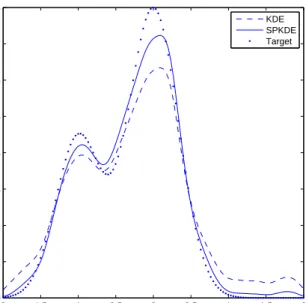
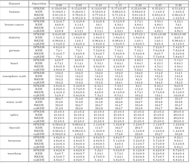
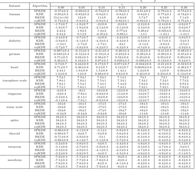
3.2.1 SPKDE Decontamination . . . 50 3.3 Experiments . . . 51 3.3.1 Synthetic Data . . . 51 3.3.2 Datasets . . . 52 3.3.3 Performance Criteria . . . 52 3.3.4 Methods . . . 54 3.3.5 Results . . . 54
IV. An Operator Theoretic Approach to Nonparametric Mixture Models . . . 56
4.1 Problem Setup . . . 56
4.2 Main Results . . . 59
4.3 Tensor Products of Hilbert Spaces . . . 63
4.3.1 Overview of Tensor Products . . . 63
4.3.2 Tensor Rank . . . 65
4.3.3 Some Results for Tensor Product Spaces . . . 65
4.4 Proofs of Theorems . . . 66
4.5 Identifiability and Determinedness of Mixtures of Multinomial Distributions . . . 85
4.6 Meta-Algorithms . . . 90
4.6.1 Spreading the eigenvalue gaps for categorical distri-butions . . . 96
4.6.2 Recovery Algorithm For Discrete Spaces . . . 98
4.6.3 Consistency of Recovery Algorithm . . . 103
4.6.4 Experiments . . . 105
4.6.5 Proposed Algorithm Experiments . . . 106
4.6.6 Competing Algorithms . . . 107
4.6.7 Results . . . 107
V. Future Work, Discussion, and Conclusion . . . 108
5.1 Robust Kernel Density Estimator Consistency . . . 108
5.2 Scale and Project Kernel Density Estimator . . . 110 5.3 An Operator Theoretic Approach to Nonparametric Mixture
5.3.1 Future Work Related to the Recovery Algorithm . 111
5.3.2 Additional Identifiability Results . . . 111
5.3.3 Potential Statistical Test and Estimator . . . 112
5.3.4 Identifiability and the Value 2n−1 . . . 113
5.4 Conclusion . . . 113
APPENDICES . . . 115
A.1 Proofs . . . 116
A.2 Experimental Results . . . 125
B.1 Additional Proofs . . . 127
B.2 Spectral Algorithm for Linearly Independent Components . . 134
LIST OF FIGURES
Figure
3.1 Density with contamination satisfying Assumption A . . . 44
3.2 Infinite sample SPKDE transform. Arrows indicate the area under the line. . . 45
3.3 Infinite sample version of the level set rejection KDE . . . 47 3.4 KDE and SPKDE in the presence of uniform noise . . . 51
LIST OF TABLES
Table
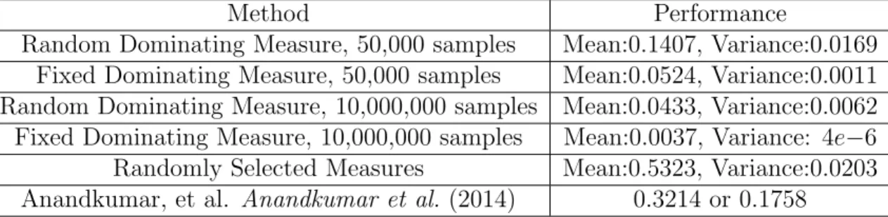
3.1 Wilcoxon signed rank test results . . . 55
4.1 Experimental Results . . . 107 A.1 Mean and Standard Deviation of DKL
b f||f0
. . . 125 A.2 Mean and Standard Deviation of DKL
f0||fb
LIST OF APPENDICES
Appendix
A. Chapter III Additional Proofs and Experimental Results . . . 116
ABSTRACT
Functional Analytic Perspectives on Nonparametric Density Estimation by
Robert A. Vandermeulen
Chair: Clayton Scott
Nonparametric density estimation is a classic problem in statistics. In the standard estimation setting, when one has access to iid samples from an unknown distribution, there exist several established and well-studied nonparametric density estimators. Yet there remains interesting alternative settings which are less well-studied. This work considers two such settings. First we consider the case where the data contains some contamination, i.e. a portion of the data is not distributed according to the density we would like to estimate. In this setting one would like an estimator which is robust to the contaminating data. An approach to this was suggested inKim and Scott (2012). The estimator in that paper was analytically and experimentally shown to be robust, but no consistency result was presented. In Chapter II it is demonstrated that this estimator is indeed consistent for a class of convex losses. Chapter III introduces a new robust kernel density estimator based on scaling and projection in Hilbert space. This estimator is proven to be consistent and will converge to the true density provided certain assumptions on the contaminating distribution. Its efficacy is demonstrated experimentally by applying it to several datasets. Chapter IV considers a different setting which can be thought of as nonparametric mixture modelling. Here one would
like to estimate multiple densities with access to groups of samples where each sample in a group is known to be distributed according the same unknown density. Tight identifiability bounds and a highly general algorithm for recovery of the densities are presented for this setting.
Functional analysis is a unifying theme of these problems. Hilbert spaces in partic-ular are used extensively for the construction of estimators and mathematical analysis.
CHAPTER I
Introduction
There are two major thrusts of research presented in this thesis and they will be introduced separately.
1.1
Kernel Density Estimation
Density estimation is one of the oldest problems in statistics. Given data one would like to estimate its underlying distribution. Oftentimes the data is known to come from a parametric class of distributions, such as the class Gaussian distributions. In this case one simply needs to estimate the parameters of the distribution. When the data come form a class which is too complicated to effectively model, or perhaps wholly unknown distribution, one resorts to using a nonparametric density estimator. There are several examples of such estimators, but arguably the most commonly used estimator is the kernel density estimator. The estimator is as follows. Letf :Rd→
R
be a pdf and X1, . . . , Xn be iid samples from f. Let kσ(x, x0) be a radial smoothing
kernel of the form kσ(x, x0) =σ−dq(kx−x0k2/σ) for some function q ≥0 such that
q(k·k2) is a pdf on Rd. Then ¯ fσn := 1 n n X i=1 kσ(·, Xi)
is the well-known kernel density estimator (KDE) (Silverman (1986), Scott (1992), Devroye and Lugosi (2001)).
This estimator has many desirable properties. Foremost it is universally consis-tent. If we allow n → ∞ and σ → 0 with a rate satisfying nσd → ∞ then we have
thatf−f¯n σ
p
→0 in both the 1 and 2 normsDevroye and Lugosi (2001). With more restrictive assumptions on the kernel, densityf, and rate onσthe consistency extends further to the ∞norm Gin´e and Guillou (2002). The KDE also avoids boundary is-sues associated with another popular nonparametric density estimator, the histogram Silverman (1986).
One issue with kernel density estimators is a lack of robustness. This work contains two major contributions to the problem of robust kernel density estimation. The first contribution is proving the consistency of a previously proposed robust kernel density estimator.
1.1.1 Consistency of The Robust Kernel Density Estimator
In Kim and Scott (2012) the authors suggest a modification of the KDE to in-duce robustness. In order to construct this estimator we additionally assume that kσ is positive-semidefinite. Thus kσ(x, x0) = hΦσ(x),Φσ(x0)iHσ, where Hσ is the
reproducing kernel Hilbert space (RKHS) associated withkσ (Aronszajn, 1950), and
Φσ(x) := kσ(·, x) is the canonical feature map (Steinwart and Christmann, 2008).
Some kernels satisfying these properties include the multivariate Gaussian, Laplacian, and Student kernels.
With this notation, the KDE may be written as
¯ fσn= 1 n n X i=1 Φσ(Xi),
solution of a least squares problem ¯ fσn = argmin g∈Hσ 1 n n X i=1 kg−Φσ(Xi)k 2 Hσ.
Replacing the squared loss with a robust lossρ, yields arobust kernel density estima-tor: fσn = argmin g∈Hσ 1 n n X i=1 ρ kg−Φσ(Xi)kHσ . (1.1)
This construction was first introduced byKim and Scott (2012) where they established several properties including a representer theorem, a convergent iterative algorithm, and the influence function. The representer theorem states that
fσn= n X i=1 αiΦσ(Xi), where αi ≥0 and Pn 1αi = 1.
In this work we will establish consistency of the RKDE in theL1 norm for a class of convex losses.
1.1.2 Related Work
The consistency of kernel density estimators has been established under the L1
norm with very weak assumptions on distribution and kernel (Devroye and Lugosi, 2001). Necessary conditions on n and σ for L1 consistency of the KDE are n → ∞ with σ → 0 and rate on bandwidth nσd → ∞. Sup-norm consistency has also been established for a less general class of kernels and densities requiring more restrictive regularity conditions (Silverman (1978), Stute (1982), Einmahl and Mason (2000), Deheuvels (2000),Gin´e and Guillou (2002), Gine et al. (2004),Wied and Weissbach (2012)).
Consistency proofs tend to proceed by decomposing the error into a stochastic estimation error and a non-stochastic approximation error, namely
f¯σn−f ≤ f¯σn−f¯σ + f¯σ −f , Where ¯fσ = R kσ(·, x)f(x)dx = R
Φσ(x)f(x)dx. The right summand is shown to
go to zero analytically and the left summand is shown to go to zero with techniques from empirical process theory. We will show a simple proof of the consistency of the KDE using this decomposition and Bennett’s inequality for Hilbert space to control the stochastic term. However, this decomposition is less fruitful for the RKDE, for which fσ does not have a closed form expression (see Section 5.1). Instead, we use
a completely different technique by investigating the convergent iterative algorithm used to compute the RKDE in Kim and Scott (2012).
1.1.3 Scale and Project Kernel Density Estimator
In Chapter III we introduce a new robust kernel density estimator. We consider the situation where most observations come from a target density ftar but some
observations are drawn from a contaminating density fcon, so our observed samples
come from the density fobs = (1−ε)ftar+εfcon. It is not known which component a
given observation comes from. When considering this scenario in the infinite sample setting we would like to construct some transform that, when applied to fobs, yields
ftar. We introduce a new formalism to describe transformations that “decontaminate”
fobs under sufficient conditions onftar andfcon. We focus on a specific nonparametric
condition onftar andfcon that reflects the intuition that the contamination manifests
in low density regions of ftar. In the finite sample setting, we seek a nonparametric
density estimator that converges toftarasymptotically. Thus, we construct a weighted
density regions. To do this we multiply the standard KDE by a real value greater than one (scale) and then find the closest pdf to the scaled KDE in the L2 norm (project),
resulting in a scaled and projected kernel density estimator (SPKDE). Because the squared L2 norm penalizes point-wise differences between functions quadratically,
this causes the SPKDE to draw weight from the low density areas of the KDE and move it to high density areas to get a more uniform difference to the scaled KDE. The asymptotic limit of the SPKDE is a scaled and shifted version of fobs. Given
our proposed sufficient conditions on ftar and fcon, the SPKDE can asymptotically
recover ftar.
In this work we present a new formalism for nonparametric density estimation, necessary and sufficient conditions for decontamination, the construction of the SP-KDE, and a proof of consistency. We also include experimental results applying the algorithm to benchmark datasets with comparisons to the RKDE, traditional KDE, and an alternative robust KDE implementation. Many of our results and proof tech-niques are novel in KDE literature.
1.2
Nonparametric Mixture Models
Chapter IV addresses a different sort of problem which is related to mixture mod-elling. A finite mixture modelP is a probability measure over a space of probability measures where P({µi}) =wi >0 for some finite collection of probability measures
µ1, . . . , µm and Pmi=1wi = 1. A realization from this mixture model first randomly
selects some mixture component µ ∼ P and then draws from µ. Mixture models have seen extensive use in statistics and machine learning.
A central theoretical question concerning mixture models is that of identifiability. A mixture model is said to be identifiable if there is no other mixture model that defines the same distribution over the observed data. Classically mixture models were concerned with the case where the observed data X1, X2, . . . are iid with Xi
distributed according to some unobserved random measure µi with µi iid ∼ P. This situation is equivalent to Xi iid ∼ Pm
j=1wjµj. If we impose no restrictions on the
mixture components µ1, . . . , µm one could easily concoct many choices of µj and wj
which yield an identical distribution on Xi. Because of this, most previous work
on identifiability assumes some sort of structure on µ1, . . . , µm, such as Gaussianity
Anderson et al. (2014); Bruni and Koch (1985); Yakowitz and Spragins (1968). In this work we consider an alternative scenario where we make no assumptions on µ1, . . . , µm and instead have access to groups of samples that are known to come
from the same component. We will call these groups of samples “random groups.” Mathematically a random group is a random elementXi whereXi = (Xi,1, . . . , Xi,n)
with Xi,1, . . . , Xi,n iid
∼ µi and µi iid
∼P.
In this setting identifiability is now concerned with the distribution over Xi and
the value of n, the number of samples in each random group. We call a mixture of measures P n-identifiable if it is the simplest mixture model (in terms of number of mixture components) that yields the observed distribution onXi. We also introduce a
concept which is stronger than identifiability. We callP n-determinedif it is theonly mixture model that yields the observed distribution onXi. In this work we show that
every mixture model withmcomponents is (2m−1)-identifiable and 2m-determined. Furthermore we show that any mixture model with linearly independent components is 3-identifiable and 4-determined. We also show that a mixture model with jointly irreducible components is 2-determined. These results hold for any mixture model over any space and cannot be improved. Finally, using these results, we demonstrate some new and old results on the identifiability of multinomial mixture models.
We also include algorithms for the recovery of the mixture components culmi-nating in a algorithm for the recovery of mixtures of categorical distributions with m arbitrary mixture components provided 2m −1 samples per group. We include experimental results showing that this algorithm does indeed recover the mixture
components from data.
1.2.1 Previous Work
In classical mixture model theory identifiability is achieved by making assumptions about the mixture components. Some assumptions which yield identifiability are Gaussian or binomial mixture components Bruni and Koch (1985); Teicher (1963). If one makes no assumptions on the mixture components then one must leverage some other type of structure in order to achieve identifiability. An example of such structure exists in the context of multiview models. In a multiview model samples have the form Xi = (Xi,1, . . . , Xi,n) and the distribution of Xi is defined by
Pm i=1wi Qn j=1µ j i.
InAllman et al.(2009) it was shown that ifµji are probability distributions onRwith µj1, . . . , µjm linearly independent for all j and n ≥3, then the model is identifiable.
The setting which we investigate is a special case of the multiview model where µji = µji0 for all i, j, j0. If the sample space of the µi is finite then this problem is
exactly the topic modelling problem with a finite number of topics and one topic for each document. In topic modelling each µi is a “topic” and the sample space is a
finite collection of words. This setting is well studied and it has been shown that one can recover the true topics provided certain assumptions on the topics Allman et al. (2009); Anandkumar et al. (2014); Arora et al. (2012). This problem was studied for arbitrary topics in Rabani et al. (2014). In this paper the authors introduce an algorithm that recovers any mixture ofmtopics provided 2m−1 words per document. They also show, in a result analogous to our own, that this 2m−1 value cannot be improved. Our proof techniques are quite different than those used in Rabani et al. (2014), hold for arbitrary sample spaces, and are less complex. Additional connections to previous work are given in Chapter IV.
CHAPTER II
Consistency of Robust Kernel Density Estimators
In this chapter we present a proof of the consistency of the robust kernel density estimator (RKDE) described in Kim and Scott (2012). First we will introduce the statistical setting for the estimator and quickly review the classic kernel density es-timator (KDE). Next we demonstrate a new proof of the consistency of the KDE. Components of this proof will be useful for proving the consistency of the RKDE. Af-ter this we introduce the RKDE and a few results from Kim and Scott (2012). Then we will prove the consistency of the RKDE. For readability many of the lemmas will only include proof sketches and full proofs can be found at the end of the chapter.
Letf :Rd →Rbe a pdf andX1, . . . , Xnbe iid samples fromf. Letkσ(x, x0) be a
radial smoothing kernel of the formkσ(x, x0) =σ−dq(kx−x0k2/σ) for some function
q≥0 such that q(k·k2) is a pdf onRd. Then
¯ fσn := 1 n n X i=1 kσ(·, Xi)
is the well-known KDE (Silverman (1986),Scott (1992),Devroye and Lugosi (2001)). We will additionally assume that kσ is positive semi-definite. Thus kσ(x, x0) =
hΦσ(x),Φσ(x0)iHσ, where Hσ is the reproducing kernel Hilbert space (RKHS)
can be represented as ¯ fσn= 1 n n X i=1 Φσ(Xi).
Using basic techniques from calculus of variations it is straightforward to show that the KDE is equal to the minimizer of a least squares problem
¯ fσn= arg min g∈Hσ 1 n n X i=1 kg−Φσ(Xi)k 2 Hσ.
By replacing the squared loss with a robust loss ρwe arrive at the RKDE from Kim and Scott (2012) arg min g∈Hσ 1 n n X i=1 ρ kg−Φσ(Xi)kHσ .
Note that for radial kernels we have
kΦσ(x)kHσ =
q
σ−dq(kx−xk 2/σ)
=pq(0)σ−d/2
which does not depend on x. Because of this, we will abuse notation slightly and let kΦσkHσ ,kΦσ(x)kHσ. Note that as σ →0, kΦσkHσ grows without bound, a fact we
will use frequently. Throughout this chapterσ will implicitly be a function ofn, such that σ →0 as n→ ∞. We will use fn
σ to denote the RKDE for a general loss ρ and
¯ fn
σ to denote the special case corresponding to ρ(·) = (·) 2
2.1
Novel KDE Consistency Proof
First we will introduce a construction that will be used frequently throughout the chapter: Dσ = Z Φσ(x)dν(x) ν is a probability measure .
Note that this and all Hilbert space valued integrals are Bochner integrals; see Stein-wart and Christmann (2008) for a basic introduction to Bochner integrals. For this chapter these integrals can be thought of as the convolution of the kernel with a mea-sure. This in turn implies that all elements of Dσ are pdfs. In fact all of the density
estimators in this chapter will be an element of some Dσ.
We will now present a novel proof ofL1 consistency of the kernel density estimator.
Theorem II.1. If n → ∞ and σ →0 with nσd→ ∞ then
f¯σn−f 1 p →0. Proof. Let ¯fσ =EX∼f [Φσ(X)]. By the triangle inequality we have
f −f¯σn 1 ≤ f−f¯σ 1+ f¯σn−f¯σ 1.
The left term in the sum goes to zero by elementary analysis (Devroye and Lugosi, 2001). We only need to show that f¯σn−f¯σ
1 p
→0. First we show convergence in the RKHS.
Lemma II.2. Let ε >0. For sufficiently small σ,
P f¯σn−f¯σ Hσ ≥ε ≤exp ( − nε 2 4kΦσk2Hσ ) .
Therefore if n → ∞ and σ →0 with nσd→ ∞, then f¯σn−f¯σ
Hσ
p
Proof Sketch. Observe that Ef¯σn =E " 1 n n X 1 Φσ(Xi) # =EX∼f[Φσ(X)] = ¯fσ.
This fact combined with Bennett’s inequality for Hilbert space yields the inequality in the lemma, after some trivial manipulations. The second part of the lemma is a simple consequence of the inequality.
The previous lemma follows from Bennett’s inequality for Hilbert space, but Ho-effding’s or Bernstein’s inequality for Hilbert space would also suffice (Pinelis, 1994). For other examples of simple proofs using concentration inequalities see Caponnetto and Vito (2007) and Bauer et al. (2007). The next lemma allows us to bound L1
norms over sets of finite Lebesgue measure. Let λ denote Lebesgue measure.
Lemma II.3. Let S ∈Rd be a set with finite Lebesgue measure and g ∈ H
σ. Then
Z
S
|g(x)|dx≤2pλ(S)kgkHσ .
Proof Sketch. We will present a proof for the situation where g >0. For the general case we can split the following integral into two parts corresponding to the subsets of
S whereg is positive and g is negative. We have, Z S g(x)dx 2 = Z S hΦσ(x), giHσdx 2 = * Z S Φσ(x)dx, g + Hσ 2 ≤ Z S Φσ(x)dx 2 Hσ kgk2Hσ = Z S Z S hΦσ(x),Φσ(x0)iHσdxdx 0kgk2 Hσ = Z S Z S kσ(x, x0)dxdx0kgk2Hσ ≤ Z S 1dxkgk2Hσ =λ(S)kgk2Hσ.
For pdfs embedded in RKHSs, Lemma II.3 allows us to show thatHσ convergence
implies L1 convergence.
Lemma II.4. Let f : Rd →
R be a pdf and gσn and hnσ be sequences of (possibly
random) densities in a sequence of spaces Dσ (again σ is implicitly a function of n).
If kgn σ −fk1 p →0 and kgn σ −hnσkHσ p →0 then kgn σ −hnσk1 p →0 .
Proof Sketch. Define B(y, r) to be the open ball centered at y with radius r and χS
to be the indicator function on the set S. Let ε > 0. Choose r large enough that R
and B(0, r)C partition Rd we have kgn σ −h n σk1 = (g n σ −h n σ) χB(0,r)+χB(0,r)C 1 =(gnσ −hnσ)χB(0,r) 1+ (g n σ −h n σ)χB(0,r)C 1. (2.1)
The left summand goes to zero in probability by Lemma II.3 so it becomes bounded by ε/3 with probability going to one. Since
(f−g n σ)χB(0,r)C 1 p →0 we have g n σχB(0,r)C 1 p → f χB(0,r)C 1 < ε/3. Since g n
σ and hnσ are densities and both of
them are converging to have the same amount of mass in B(0, r), their mass in B(0, r)C must also be converging. This means
h n σχB(0,r)C 1 − g n σχB(0,r)C 1 p →0 so h n σχB(0,r)C
1 becomes bounded byε/3 with probability going to one. Thus the right
summand of (2.1) becomes bounded by 2ε/3 with high probability. Putting these results together we havekgn
σ −hnσk1 < ε with probability going to one.
The previous lemma is a bit more general than is necessary for the current theorem, but it will be handy later. In this casegn
σ in the last lemma is replaced by ¯fσ andhnσ
is replaced with ¯fn
σ, thus completing our proof of Theorem II.1.
It is worth noting that Lemma II.2 also implies consistency with respect to L2 and L∞ norms, assuming suitable conditions ensuring that the approximation error goes to zero. L2 consistency is implied as long as k
σ(·, x) ∈ L2 Rd
for all x ∈ Rd,
(in particular, kσ need not be a reproducing kernel) because Lemma II.2 holds for
general Hilbert spaces. L∞ consistency follows from the Cauchy-Schwarz inequality,
f¯σn(x)−f¯σ(x) = Φσ(x),f¯σn−f¯σ Hσ ≤ kΦσkHσ f¯σn−f¯σ H σ .
band-width, nσ2d→ ∞.
2.2
RKDE Consistency
We begin by reviewing some results about the RKDE.
2.2.1 Previous Results
Before we prove consistency of the RKDE, we will introduce some additional technical background on the RKDE from Kim and Scott (2012). First we will define some properties ρ may have. Let ρ : [0,∞)→ [0,∞), ψ , ρ0, and ϕ(x) , ψ(x)/x. Consider the following properties:
(B1) ρ is strictly convex
(B2) ρ is strictly increasing,ρ(0) = 0 and ρ(x)/x→0 as x→0 (B3) ϕ(0) := limx→0 ψ(x)x exists and is finite
(B4) ψ is bounded
(B5) ρ00 exists and is nonincreasing on (0,∞) (B6) ϕis nonincreasing.
Some examples of losses satisfying all of these properties areρ(x) = √x2+ 1−1,
ρ(x) =xarctan (x), andρ(x) =x−log (1 +x). It is easy to show that property (B1) guarantees the existence and uniqueness offn
σ (Kim and Scott, 2012). Let f be a pdf
and X1,· · · , Xn be iid samples fromf. Let Jσn(·) be the empirical risk introduced in
(1.1). Taking the Gateaux derivative of the risk gives us
δJσn(g;h) =− * 1 n n X 1 ϕ kΦσ(Xi)−gkHσ (Φσ(Xi)−g), h + Hσ .
If (B2) and (B3) are satisfied then a necessary condition for g = fn
σ is that the
Gateaux derivative atg is 0 for all directions h, which is equivalent to left term in the inner product being 0 (Lemma 1Kim and Scott (2012)). A straightforward algebraic
manipulation of the last condition gives us Pn 1ϕ kΦσ(Xi)−gkHσ Φσ(Xi) Pn 1 ϕ kΦσ(Xj)−gkHσ =g. With this in mind we introduce the following functional,
Rnσ :Hσ → Hσ :g 7→Rnσ(g) = R ϕ kΦσ(x)−gkHσ Φσ(x)dµn(x) R ϕ kΦσ(y)−gkHσ dµn(y) = n X 1 αi(g)kσ(·, Xi) where αi(g) = ϕ kΦσ(Xi)−gkHσ Pn 1 ϕ kΦσ(Xj)−gkHσ
and µn is the empirical measure corresponding to the sample. This function is the
Iterated Reweighted Least Squares algorithm (IRWLS) from Kim and Scott (2012), which is used to compute the RKDE in practice. From Corollary 6 inKim and Scott (2012) it is easy to show that if (B1), (B2), (B3), (B5), and (B6) are satisfied (note that (B4) is used later), the sequence {Rn
σ(0), Rnσ(Rσn(0)), . . .} converges in Hσ to
fn
σ, which is the unique fixed point of Rnσ.
2.2.2 Consistency Theorem and Proof
Theorem II.5. Let f ∈L2 Rdand letρ satisfy (B1)-(B6). Ifnσd→ ∞and σ→0
as n → ∞ then kfn σ −fk1
p
→0.
We know that ψ is bounded by (B4). In the proofs that follow it will be assumed, for simplicity, that supxψ(x) = 1. Note that any loss with boundedψ can be adapted such that supxψ(x) = 1. This is done by dividingρby supxψ(x) and does not affect the RKDE. The longer and more technical proof sketches are contained in a subsection
after this one.
The following lemma helps us establish the behavior of elements inDσ with large
norms.
Lemma II.6. For all g ∈ Dσ, kgk
2
Hσ ≤ kgk∞.
Proof. By the definition of Dσ, let g =
R
Φσ(x)dν(x), where ν is a probability
mea-sure. kgk2Hσ =hg, giHσ = Z Φσ(x)dν(x), g Hσ = Z hΦσ(x), giHσdν(x) = Z g(x)dν(x)≤ Z kgk∞dν(x) =kgk∞.
This lemma allows us to show that an element in Dσ with large norm will have
most of its mass concentrated around one point. An element ofDσ having most of the
mass around one point causes its general risk to be large. The Vapnik-Chervonenkis inequality allows us to show that all such elements will, with high probability, have high empirical risk.
Lemma II.7. If σ →0 and n→ ∞ then P kfn
σk 2 Hσ ≥ 9 10kΦσk 2 Hσ →0. The constant 9
10 was chosen simply for convenience, it could be replaced with any
positive value less than one.
The following result will be used to prove Lemma II.9 and Theorem II.5.
Lemma II.8. f¯σ
Hσ ≤ kfk2.
Lugosi, 2001) we have f¯σ 2 Hσ = Z f(x)Φσ(x)dx, Z f(y)Φσ(y)dy Hσ = Z f(x) Φσ(x), Z f(y)Φσ(y)dy Hσ dx = Z f(x) (f ∗kσ) (x)dx =hf, f ∗kσi2 ≤ kfk2kf ∗kσk2 ≤ kfk2kfk2kkσk1 =kfk22.
Lemma II.7 shows thatfn
σ is, with high probability, in a ball of radius
q
9
10kΦσkHσ.
Lemma II.9 shows that, on that ball, Rn
σ is a contraction mapping.
Lemma II.9. Let n → ∞, σ → 0, and nσd → ∞. There exists CR such that, with
probability going to one, the restriction of Rnσ to BHσ
0, q 9 10kΦσkHσ is Lipschitz continuous with Lipschitz constant CRkΦσk
−1
Hσ.
This lemma is the final key to proving Theorem II.5.
Proof of Theorem II.5. Using the triangle inequality we get
kf −fσnk1 ≤ f−f¯σn 1+ f¯σn−fσn 1.
We know the left term of the summand goes to zero in probability by Theorem II.1, so it is sufficient to show that the right summand goes to zero in probability. By Lemma II.4 it is sufficient to show that fn
σ −f¯σn
Notice that Rn
σ(0) = ¯fσn and recallRσn(fσn) =fσn. Using Lemma II.7 and II.9, with
probability going to 1, the following holds
f¯σn−fσn H σ =kR n σ(0)−Rnσ(fσn)kHσ ≤ kfn σ −0kHσ kΦσk −1 HσCR < r 9 10kΦσkHσkΦσk −1 HσCR = r 9 10CR. Since f¯σn−f¯σ H σ p →0 and f¯σ H
σ ≤ kfk2 <∞ (by Lemma II.8), for arbitrary
s > 0 we have f¯σn
Hσ < kfk2 +s with probability going to one. Applying the contraction mapping steps again we get, with probability going to 1, that
f¯σn−fσn Hσ =kR n σ(0)−R n σ(f n σ)kHσ ≤ kfn σ −0kHσ kΦσk −1 Hσ CR ≤fσn−f¯σnH σ + f¯σn H σ kΦσk −1 HσCR ≤ r 9 10CR+kfk2+s ! kΦσk −1 Hσ CR.
The last line goes to zero as σ →0, completing our proof.
2.2.3 Proof Sketches
Proof Sketch of Lemma II.7. We know that fσn ∈ Dσ, so to prove this lemma we will
show that as n → ∞ and σ → 0, all vectors in Dσ with Hσ-norm greater than or
equal to q9
10kΦσkHσ will have empirical risk greater than the zero vector. Define
Jn
σ :Hσ →R as the empirical risk function
Jσn(g) = 1 n n X 1 ρ kΦσ(Xi)−gkHσ .
Letgn
σ be the minimizer ofJσnwhen restricted to vectors inDσ withHσ-norm greater
than or equal toq109 kΦσkHσ. By Lemma II.6 there must existx
∗ such thatgn σ(x ∗)≥ 9 10kΦσk 2
Hσ, this causes most of of the mass ofgnσ to reside nearx
∗. It is possible to show
that, given any r > 0 and ε > 0, for sufficiently small σ, that supx∈B(x∗,r)Cgnσ(x) <
3 20kΦσk
2
Hσ +ε. As n gets large, Jσn becomes well approximated by Jσ where
Jσ(g) =
Z
ρ kΦσ(x)−gkHσ
f(x)dx. (2.2)
We will substitute Jσ for Jσn (in the formal proof we work with Jσn and invoke the
VC inequality to relate it to the population risk). Since ρ is increasing, the following holds for sufficiently small σ,
Jσ(gnσ)≥ Z B(x∗,r)C ρ kΦσ(x)−gσnkHσ f(x)dx ≥ Z B(x∗,r)C ρ q kΦσk 2 Hσ −2hgσn,Φσ(x)iHσ +kgσnk 2 Hσ f(x)dx ≥ Z B(x∗,r)C ρ s kΦσk2Hσ −2 3 20kΦσk 2 Hσ +ε +kgn σk 2 Hσ ! f(x)dx.
Since ε can be set to be arbitrarily small and kgn σk
2
Hσ ≥ 109 kΦσk 2
Hσ the last term has
an approximate lower bound of
& Z B(x∗,r)C ρ r kΦσk 2 Hσ − 6 20kΦσk 2 Hσ + 9 10kΦσk 2 Hσ ! f(x)dx ≥ρ kΦσkHσ r 32 20 ! inf y Z B(y,r)C f(x)dx.
Finally r can be chosen to be sufficiently small so that infy
R
B(y,r)Cf(x)dx is
arbi-trarily close to one. Thus as n→ ∞ and σ →0, with probability going to one
Jσn(gσn)&ρ kΦσkHσ r 32 20 ! .
Now, notice that
Jσn(0) = 1 n n X 1 ρ kΦσ(Xi)−0kHσ =ρ kΦσkHσ .
It then follows that, with probability going to one, Jn
σ (gnσ)> Jσn(0).
Proof Sketch of Lemma II.9. Letg, h∈BHσ
0,q109 kΦσkHσ . We have kRn σ(g)−R n σ(h)kHσ = R ϕ kΦσ(x)−gkHσ Φ (x)dµn(x) R ϕ kΦσ(y)−gkHσ dµn(y) − R ϕ kΦσ(x0)−hkHσ Φ (x)dµn(x0) R ϕ kΦσ(y0)−hkHσ dµn(y0) Hσ . (2.3)
Note that all integrals are over the same measure. Consider the situation if the integrals were evaluated at one point, we have that
ϕ kΦσ(x)−gkHσ ϕ kΦσ(y)−gkHσ − ϕ kΦσ(x)−hkHσ ϕ kΦσ(y)−hkHσ (2.4) = N ϕ kΦσ(y)−gkHσ ϕ kΦσ(y)−hkHσ
where N =ϕ kΦσ(x)−gkHσ ϕ kΦσ(y)−hkHσ . . . −ϕ kΦσ(x)−hkHσ ϕ kΦσ(y)−gkHσ .
We will now find a lower bound on the denominator. Note that sinceg and h live in BHσ 0,kΦσkHσ q 9 10
, thatkΦσ(y)−gkHσ and kΦσ(y)−gkHσ grow without bound
as σ → 0. Since ρ is convex ψ must be increasing and since ψ has a supremum of 1, ψ(z) is well approximated by 1 for large z. Thus we have, for small σ that the denominator is well approximated as follows
ϕ kΦσ(y)−gkHσ ϕ kΦσ(y)−hkHσ =ψ kΦσ(y)−gkHσ kΦσ(y)−gkHσ ψ kΦσ(y)−hkHσ kΦσ(y)−hkHσ ≈ 1 kΦσ(y)−gkHσkΦσ(y)−hkHσ ≥ 1 kΦσk 2 Hσ 1 +p9/10 2 =CDkΦσk −2 Hσ where CD = 1 +p9/10 −2
. We will now find an upper bound on the numerator. By the triangle inequality
ϕ kΦσ(x)−gkHσ ϕ kΦσ(y)−hkHσ . . . −ϕ kΦσ(x)−hkHσ ϕ kΦσ(y)−gkHσ ≤ ϕ kΦσ(x)−gkHσ ϕ kΦσ(y)−hkHσ . . . −ϕ kΦσ(x)−gkHσ ϕ kΦσ(y)−gkHσ . . . +ϕ kΦσ(x)−gkHσ ϕ kΦσ(y)−gkHσ . . . −ϕ kΦσ(x)−hkHσ ϕ kΦσ(y)−gkHσ .
Consider the second summand, ϕ kΦσ(x)−gkHσ ϕ kΦσ(y)−gkHσ . . . (2.5) −ϕ kΦσ(x)−hkHσ ϕ kΦσ(y)−gkHσ =ϕ kΦσ(y)−gkHσ ϕ kΦσ(x)−gkHσ −ϕ kΦσ(y)−hkHσ ≤ 1 kΦσ(y)−gkHσ ϕ kΦσ(x)−gkHσ −ϕ kΦσ(x)−hkHσ ≤ 1 kΦσkHσ 1−q9 10 ϕ kΦσ(x)−gkHσ −ϕ kΦσ(x)−hkHσ .
Just asϕ(z) becomes well approximated by 1z for largez,ϕ0(z) becomes well approx-imated by −z21. Using this it can be shown that there existsCL>0 such that, for suffi-ciently small σ, ϕ kΦσ(y)− · kHσ
is Lipschitz continuous onBHσ 0,q9 10kΦσkHσ with Lipschitz constant kΦσk
−2 HσCL. Now we have ϕ kΦσ(x)−gkHσ −ϕ kΦσ(x)−hkHσ ≤ kg−hkHσ kΦσk −2 Hσ CL.
It now follows that (2.5) is less than or equal tokΦσk
−3
HσCN for someCN >0.
Return-ing to (2.4), we can now show that it has an upper bound of 2kΦσk −3 HσCN kΦσk−H2σCD =kΦσk −1 Hσ 2CN CD .
This generally describes the behavior of the values found in (2.3). To take care of the R
Φσ(x)dµn(x) terms, note that by Theorem II.1
R Φσ(x)dµn(x)−f¯σ Hσ p →0 if nσd→ ∞. By Lemma II.8, f¯σ H σ ≤ kfk2 so R Φσ(x)dµn(x) H σ becomes bounded
with high probability, thus completing our proof sketch.
2.3
Proofs of Lemmas
For convenience the proofs have been split up into two subsections, one for proofs from the KDE section and the other for proofs from the RKDE section.
2.3.1 KDE Consistency Proofs
The following lemma is a Hilbert space version of Bennett’s inequality (Smale and Zhou, 2007) and will be used in the proof of Lemma II.2.
Lemma II.10. Let H be a Hilbert space and {ξi}mi=1 be m (m < ∞) independent
random variables with values in H. Also, assume that for each i, kξikH ≤ B < ∞
almost surely. Let δ2 =Pm
i=1E[kξik 2 H]. Then P 1 m m X i=1 (ξi−E[ξi]) H ≥ε ! ≤exp −mε 2B log 1 + mBε δ2 ,∀ε >0.
Proof of Lemma II.2. We will apply Lemma II.10. From the lemma statement let ξi = Φσ(Xi) and m=n yielding, for all ε >0
P f¯σn−f¯σ Hσ ≥ε ≤exp ( − nε 2kΦσkHσ log 1 + nkΦσkHσ ε nkΦσk 2 Hσ !) = exp − nε 2kΦσkHσ log 1 + ε kΦσkHσ . As σ →0 then 1 + kΦσkε Hσ
→1 so for sufficiently small σ
log 1 + ε kΦσkHσ ≥ ε 2kΦσkHσ and P f¯σn−f¯σ H σ ≥ε ≤exp ( − nε 2 4kΦσk2Hσ )
which goes to zero as n
kΦσk2Hσ → ∞, or equivalently nσd → ∞. So f¯σn−f¯σ Hσ p →0.
Proof of Lemma II.3. LetS+ ={s|s∈S, g(s)≥0} and S− =S\S+. We have Z S |g(x)|dx= Z S+ g(x)dx+ Z S− −g(x0)dx0 = Z S+ hg,Φσ(x)iHσdx+ Z S− h−g,Φσ(x0)iHσ dx 0 = * g, Z S+ Φσ(x)dx + Hσ + * −g, Z S− Φσ(x0)dx0 + Hσ ≤ kgkHσ Z S+ Φσ(x)dx Hσ + Z S− Φσ(x0)dx0 Hσ . (2.6) Now consider Z S+ Φσ(x)dx 2 Hσ = * Z S+ Φσ(x)dx, Z S+ Φσ(x0)dx0 + Hσ = Z S+ Z S+ hΦσ(x),Φσ(x0)iHσdxdx 0 = Z S+ Z S+ kσ(x, x0)dxdx0 ≤ Z S+ 1dx0 =λ(S+)
and a similar result can be shown forS−. Plugging back into (2.6) we get
Z S |g(x)|dx ≤ kgkH σ p λ(S+) +pλ(S−) ≤ kgkHσ2pλ(S).
Lemma II.11. Let f be a pdf, ε >0, and y∈Rd. There existsr >0 such that Z B(y,r) f(x)dx≥1−ε. or equivalently Z B(y,r)C f(x)dx < ε.
Proof. We will prove the second statement. Consider the following, where i∈N, Z
B(y,i)C
f(x)dx= Z
χB(y,i)C(x)f(x)dx.
Clearly as i → ∞, χB(y,i)Cf → 0 pointwise. Since χB(y,i)Cf is dominated by f,
R
χB(y,i)C(x)f(x)dx → R 0dx = 0 by the dominated convergence theorem. Thus
there exists n ∈N whereRB(y,n)Cf(x)dx < ε.
Proof of Lemma II.4. Letε > 0; by Lemma II.11 let r >0 such that f χB(0,r)C
1 <
ε/3. From Lemma II.3 we have
(gnσ −hnσ)χB(0,r) 1 p →0.
Since kgn σ −fk1 p →0, we have gn σχB(0,r) 1 p → f χB(0,r) 1, and therefore h n σχB(0,r)C 1 − f χB(0,r)C 1 = 1− hnσχB(0,r) 1 − 1− f χB(0,r) 1 = hnσχB(0,r) 1− f χB(0,r) 1 ≤ (hnσ −f)χB(0,r) 1 ≤(hnσ −gσn)χB(0,r) 1+ (gnσ −f)χB(0,r) 1 p →0. Thus, h n σχB(0,r)C 1 p → f χB(0,r)C 1 . Sincef χB(0,r)C 1 < ε/3, we have P hnσχB(0,r)C 1 ≥ε5/12 →0. (2.7)
Now to finish the proof,
P(khnσ−g n σk1 > ε) =P (hnσ −gσn)χB(0,r) 1+ (hnσ−gσn)χB(0,r)C 1 > ε ≤P (hnσ−gnσ)χB(0,r) 1 ≥ε/4 +P (hnσ−gnσ)χB(0,r)C 1 >3ε/4
We’ve already shown the left summand goes to zero, now we take care of the right term P (hnσ−gσn)χB(0,r)C 1 >3ε/4 ≤P hnσχB(0,r)C 1+ gσnχB(0,r)C 1 >3ε/4 ≤P hnσχB(0,r)C 1 ≥5ε/12 +P gnσχB(0,r)C 1 > ε/3
The left summand goes to zero by (2.7). Since g n σχB(0,r)C −f χB(0,r)C 1 →0 and f χ
< ε, with probability going to one, we have gnχ
right summand goes to zero. This completes our proof.
2.3.2 RKDE Consistency Proofs
Lemma II.12. Let f :Rd →R be a pdf. For all ε > 0, there exists s > 0 such that R
B(z,s)f(x)dx≤ε for all z ∈R d.
Proof. We will proceed by contradiction. Let {xi}
∞
1 be a sequence in Rd such that
R
B(xi,1/i)f(x)dx > ε. Clearly the sequence must be bounded or else f would not
be a pdf. Let xij be a convergent subsequence and let x
0 be its limit. Let {r
j}
∞
1
be a sequence in R+ converging to zero with B x ij,1/ij
⊂ B(x0, rj). So we have
R
B(x0,r
j)f(x)dx > ε, for all j. We know
Z B(x0,r j) f(x)dx = Z χB(x0,r j)(x)f(x)dx and f χB(x0,r
j) → 0 pointwise. Since f χB(x0,rj) is dominated by f, the dominated
convergence theorem yields
lim j→∞ Z B(x0,r j) f(x)dx = lim j→∞ Z f(x)χB(x0,r j)(x)dx = Z lim j→∞f(x)χB(x 0,r j)(x)dx = Z 0dx = 0 but RB(x0,r j)f(x)dx > ε, a contradiction.
Corollary II.13. Let f : Rd →
R be a pdf with associated measure µ, ε > 0 and
r >0. There exists s >0 such that for allx∈Rd, µ(B(x, r+s)\B(x, r))< ε.
Proof. We will omit a full proof; the general strategy is the same as the previous proof. Find a series of annuli with width decreasing to zero that have probability
greater thanε. Next find a convergent subsequence of annuli centers, let its limit be x0. Finally construct a series of annuli centered atx0 with probability measure greater than ε and width going to zero and arrive at the same contradiction.
Lemma II.14. Let s >0. If σ→0 then σ−dq(s/σ)→0.
Proof. We will proceed by contradiction. Suppose σ−dq(s/σ) does not converge to zero, then there exists C > 0 such that we can find arbitrarily small σ satisfying
σ−dq(s/σ)> C. (2.8)
It is well known that there exists Cd such that the Lebesgue measure of a ball in Rd
of radius r isCdrd. Sinceq is nonincreasing (Scovel et al., 2010) this along with (2.8)
implies that there exists arbitrarily small σ satisfying
Z B(0,s) σ−dq(kxk2/σ)dx≥ Z B(0,s) σ−dq(s/σ)dx >CdsdC
where the last term must be less than or equal to 1. Now, by Lemma II.11, there existsr > 0 such that
Z B(0,r) q(kxk2)dx= Z B(0,rσ) σ−dq(kxk2/σ)dx≥1− Cds dC 2 .
For sufficiently small σ we have 1≥ Z B(0,rσ) σ−dq(kxk2/σ)dx ≥ Z B(0,rσ) σ−dq(kx0k2/σ)dx0 + Z B(0,s)\B(0,rσ) σ−dq(kxk2/σ)dx ≥1− Cds dC 2 + Z B(0,s)\B(0,rσ) σ−dq(kxk2/σ)dx.
Because q is nonincreasing this is greater than or equal to
1−Cds dC 2 +Cd sd−(rσ)dσ−dq(s/σ). As σ → 0 , Cd sd−(rσ)d→
Cdsd, so by (2.8) we can find some σ where the last
term is greater than or equal to
1− Cds dC 2 +Cds d C2 3.
The last line is greater than 1, a contradiction.
Proof of Lemma II.7. Let conv be the convex hull operator. Define
Qnσ = conv (Φσ(X1), . . . ,Φσ(Xn)) \ BHσ 0, r 9 10kΦσkHσ !C . Clearly Qn
σ ⊂ Dσ since Φσ(Xi) is a density for all i. By the representer theorem in
Kim and Scott (2012), fσn ∈ conv (Φσ(X1), . . . ,Φσ(Xn)). We also know that fσn is
the minimizer of Jσn, whereJσn:Hσ →Ris the empirical risk function
Jσn(g) = 1 n n X i=1 ρ kΦσ(Xi)−gkHσ .
From these facts if we can show P(Jσn(0)< J n σ(g),∀g ∈Q n σ)→0
then we have proven the lemma. Since Qn
σ is compact and Jσn is continuous (Kim and Scott, 2012) the set
arg min
g∈Qn σ
Jσn(g)
contains at least one element. Letgσnbe an arbitrary minimizer ofJσnrestricted toQnσ. Letµbe the measure associated withf. From Lemma II.12 we can chooser >0 such that µ(B(x, r))≤ 1
10, for all x∈R
d. Choose s >0 such thatµB(x, r+s)C≥ 4 5,
for all x ∈ Rd. The previous statement is satisfied by finding s such that, for all x,
µ(B(x, r+s)\B(x, r))< 101, which is possible by Corollary II.13. By Lemma II.6 we know there exists x∗ such that gnσ(x∗)≥ 9
10kΦσk 2
Hσ (x
∗ is implicitly a function of
n). By the definition of Qnσ, let gσn = Pn
i=1βiΦσ(Xi) with βi ≥ 0 and
Pn
1 βi = 1.
Since gσn(x∗)≥ 9 10kΦσk
2
Hσ and q is nonincreasing we have
9 10kΦσk 2 Hσ ≤ n X i=1 βikσ(Xi, x∗) = X i:Xi∈B(x∗,r) βikσ(Xi, x∗) + X j:Xj∈B(x∗,r)C βjkσ(Xj, x∗) = X i:Xi∈B(x∗,r) βikσ(Xi, x∗) + X j:Xj∈B(x∗,r)C βjσ−dq kXj −x∗k2/σ ≤ X i:Xi∈B(x∗,r) βikΦσk2Hσ +σ −dq(r/σ)
The last line is due to the fact q must be nonincreasing (Scovel et al., 2010). From Lemma II.14 we know that σ−dq(r/σ) →0 as σ → 0 , so for sufficiently small σ we
have 17 20kΦσk 2 Hσ < X i:Xi∈B(x∗,r) βikΦσk 2 Hσ and thus 17 20 < X i:Xi∈B(x∗,r) βi. (2.9)
Again, since q nonincreasing, for sufficiently small σ
sup y∈B(x∗,r+s)C gσn(y) = sup y∈B(x∗,r+s)C n X i=1 βikσ(Xi, y) = sup y∈B(x∗,r+s)C X i:Xi∈B(x∗,r) βikσ(Xi, y) + X j:Xj∈B(x∗,r)C βjhΦσ(y),Φσ(Xj)iHσ ≤σ−dq(s/σ) + X j:Xj∈B(x∗,r)C βjkΦσk 2 Hσ.
From this, (2.9) and because σ−dq(s/σ) → 0 as σ → 0, for arbitrary ε > 0 we
have, for sufficiently small σ,
sup y∈B(x∗,r+s)C gnσ(y)< ε+ 3 20kΦσk 2 Hσ.
strictly increasing, for sufficiently small σ, Jσn(gσn) = 1 n n X i=1 ρ kΦσ(Xi)−gnσkHσ = 1 n X i:Xi∈B(x∗,r+s) ρ kΦσ(Xi)−gσnkHσ . . . + 1 n X j:Xj∈B(x∗,r+s)C ρ kΦσ(Xj)−gnσkHσ ≥ 1 n X j:Xj∈B(x∗,r+s)C ρ kΦσ(Xj)−gσnkHσ = 1 n X j:Xj∈B(x∗,r+s)C ρ q kΦσk 2 Hσ −2gnσ(Xj) +kgσnk 2 Hσ ≥ 1 n X j:Xj∈B(x∗,r+s)C ρ s kΦσk2Hσ −2 3 20kΦσk 2 Hσ +ε + 9 10kΦσk 2 Hσ ! =µn B(x∗, r+s)C ρ r kΦσk2Hσ 32 20−2ε ! ≥inf x µn B(x, r+s)Cρ r kΦσk2Hσ 32 20 −2ε ! .
Since ρ is strictly convex we know that ψ is strictly increasing. Because ψ has a supremum of 1 and is strictly increasing we know that for any 1> εψ >0 there exists
bψ such that for all x > bψ, ψ(x)>1−εψ. Then, for sufficiently small σ,
ρ r kΦσk 2 Hσ 32 20 −2ε ! = √ kΦσk2H σ 32 20−2ε Z 0 ψ(x)dx ≥ √ kΦσk2Hσ 32 20−2ε Z bψ ψ(x)dx ≥(1−εψ) r kΦσk2Hσ 32 20−2ε−bψ ! (2.10)
For sufficiently small σ we have r kΦσk 2 Hσ 32 20 −2ε ≥ kΦσkHσ r 32 20 −2ε.
Since the complements of all open balls, in this case, all balls with radius r +s, have a finite shattering dimension (Devroye and Lugosi, 2001), and by our choice of r and s we know, with probability going to one, that infxµn
B(x, r+s)C → infxµ
B(x, r+s)C≥0.8. Because of this for any εB >0 we have, with probability
going to one, that infxµn
B(x, r+s)C≥0.8−εB. Since 45
q
32
20 >1, we can choose
εψ and εB such that 45 −εB
(1−εψ)
q
32
20 > 1. Using these facts with (2.10) we
have, for sufficiently small σ, with probability going to one
Jσn(gσn)≥inf x µn B(x, r+s)C(1−εψ) r kΦσk2Hσ 32 20 −2ε−bψ ! ≥ 4 5 −εB (1−εψ) kΦσkHσ r 32 20−2ε−bψ ! >kΦσkHσ. Now consider Jσn(0) = 1 n n X i=1 ρ kΦσ(Xi)−0kHσ =ρ kΦσkHσ = kΦσkHσ Z 0 ψ(x)dx+ρ(0) ≤ kΦσkHσ Z 0 1dx =kΦσkHσ.
So as n→ ∞ and σ →0 we have P(Jσn(g n σ)≤J n σ (0))→0,
thus finishing the proof.
Proof of Lemma II.9. Let g, h ∈ Hσ such that kgk 2 Hσ ≤ 9 10kΦσk 2 Hσ and khk 2 Hσ ≤ 9 10kΦσk 2
Hσ. Cross multiplication gives us
kRn σ(g)−R n σ(h)kHσ = R ϕ kΦσ(x)−gkHσ Φσ(x)dµn(x) R ϕ kΦσ(y)−gkHσ dµn(y) − R ϕ kΦσ(x0)−hkHσ Φσ(x0)dµn(x0) R ϕ kΦσ(y0)−hkHσ dµn(y0) Hσ = A B H σ where A= Z ϕ kΦσ(x)−gkHσ Φσ(x)dµn(x) Z ϕ kΦσ(y0)−hkHσ dµn(y) − Z ϕ kΦσ(x0)−hkHσ Φσ(x0)dµn(x0) Z ϕ kΦσ(y)−gkHσ dµn(y) and B = Z ϕ kΦσ(y0)−hkHσ dµn(y0) Z ϕ kΦσ(y)−gkHσ dµn(y) .
Note that A∈ Hσ and B ∈R+. We will now find a lower bound onB. As shown in
the reverse triangle inequality kΦσ(y0)−hkHσ ≥ kΦσkHσ − khkHσ ≥ kΦσkHσ 1− r 9 10 !
which grows without bound as σ→0. So for sufficiently small σ
ϕ kΦσ(y0)−hkHσ = ψ kΦσ(y 0 )−hkHσ kΦσ(y0)−hkHσ ≥ 1 2kΦσ(y0)−hkHσ ≥ 1 2 kΦσkHσ +khkHσ ≥ 1 kΦσkHσ2 1 + q 9 10 .
A similar result can be shown for ϕ kΦσ(y)−gkHσ
, so there exists CB > 0 such
that, for sufficiently small σ,
B ≥ kΦσk
−2
HσCB.
Now we will focus on A. To make the following manipulations simpler we will let
ϕ kΦσ(z)−kkHσ
A is equal to Z Tσ(x, g) Φσ(x)dµn(x) Z Tσ(y0, h)dµn(y0) . . . − Z Tσ(x0, h) Φσ(x0)dµn(x0) Z Tσ(y, g)dµn(y) = Z Tσ(x, g) Φσ(x) Z Tσ(y0, h)dµn(y0) . . . −Tσ(x, h) Φσ(x) Z Tσ(y, g)dµn(y) dµn(x) = Z Φσ(x) " Tσ(x, g) Z Tσ(y0, h)dµn(y) . . . −Tσ(x, h) Z Tσ(y, g)dµn(y) # dµn(x) = Z Z Φσ(x) Tσ(x, g)Tσ(y, h)−Tσ(x, h)Tσ(y, g) dµn(y)dµn(x).
We will now bound the inner term. Using the triangle inequality we have
Tσ(x, g)Tσ(y, h)−Tσ(x, h)Tσ(y, g) (2.11) <Tσ(x, g)Tσ(y, h)−Tσ(x, g)Tσ(y, g) + Tσ(x, g)Tσ(y, g)−Tσ(x, h)Tσ(y, g) =Tσ(x, g) Tσ(y, h)−Tσ(y, g) +Tσ(y, g) Tσ(x, g)−Tσ(x, h) .
bound the first summand. ϕ kΦσ(y)−gkHσ = ψ kΦσ(y)−gkHσ kΦσ(y)−gkHσ ≤ 1 kΦσ(y)−gkHσ ≤ 1 kΦσkHσ − kgkHσ ≤ 1 kΦσkHσ 1−q9 10 . (2.12)
A similar result can be shown for ϕ kΦσ(x)−gkHσ
. Consider z ≥ kΦσkHσ 1−q9 10 , then |ϕ0(z)|= ψ(z) z 0 = zψ0(z)−ψ(z) z2 ≤ |zψ 0(z)|+|ψ(z)| z2 .
We will now analyze the behaviour of ψ0, specifically, there exists sufficiently large r such that ψ0(x) ≤ 1
x for all x ≥ r. We will proceed by contradiction. Suppose this
is not the case. Then there exist positive numbers t1, t2 and t3 such that ψ0(ti)> t1i
and ti
ti+1 <
1
3. We know ψ
is bounded above by 1 so 1≥ ∞ Z 0 ψ0(x)dx ≥ t2 Z t1 ψ0(x)dx+ t3 Z t2 ψ0(y)dy ≥ t2−t1 t2 +t3−t2 t3 ≥2− 2 3,
a contradiction. From this we have that for sufficiently large z,
|zψ0(z)|+|ψ(z)| z2 ≤ z1z + 1 z2 = 2 z2.
Thus, for sufficiently small σ, on the spaceh1−q9 10
kΦσkHσ,∞
, ϕ is Lipschitz continuous with Lipschitz constant 21−q9
10 −2 kΦσk −2 Hσ. Therefore we have |ϕ(kΦσ(x)−gk)−ϕ(kΦσ(x)−hk)| ≤ kΦσ(x)−gkHσ − kΦσ(x)−hkHσ 2 1− r 9 10 !−2 kΦσk −2 Hσ ≤ kg−hkHσ 2 1− r 9 10 !−2 kΦσk −2 Hσ .
Combining the last inequality with (2.12) we have that for sufficiently smallσ, (2.11) is less than or equal to
4kg−hkHσ 1− r 9 10 !−3 kΦσk −3 Hσ .
Using this bound we can do the following. Let τ ,Tσ(x, g)Tσ(y, h)−Tσ(x, h)Tσ(y, g) , and τ0 , Tσ(x0, g)Tσ(y0, h)−Tσ(x0, h)Tσ(y0, g) , and κ,4kg−hkHσ 1− r 9 10 !−3 kΦσk −3 Hσ , we have kAk2H σ = Z Z Φσ(x)τ dµn(x)dµn(y) 2 Hσ = Z Z Φσ(x)τ dµn(x)dµn(y), Z Z Φσ(x0)τ0dµn(x0)dµn(y0) Hσ = Z Z Z Z τ τ0hΦσ(x),Φσ(x0)iHσdµn(y)dµn(y0)dµn(x)dµn(x0).
Since hΦσ(x),Φσ(x0)iHσ ≥ 0 for all x, x
0, for sufficiently small σ, the last line is less
than or equal to Z Z Z Z κ2hΦσ(x),Φσ(x0)iHσdµn(y)dµn(y0)dµn(x)dµn(x0) = Z Z κ2hΦσ(x),Φσ(x0)iHσdµn(x)dµn(x0) =κ2 Z Φσ(x)dµn(x) 2 Hσ .
Returning to the original notation, this means, for sufficiently small σ
kAkH σ ≤ Z Φσ(x)dµn(x) Hσ 4kg −hkH σ 1− r 9 10 !−3 kΦσk −3 Hσ.
From our proof of the consistency of the KDE we know that Z Φσ(x)dµn(x)−f¯σ H σ p →0
and from Lemma II.8 f¯σ
Hσ ≤ kfk2 so R Φσ(x)dµn(x) Hσ is bounded by some constant with probability going to one. Note that this is the only probabilistic step, which does not depend on g or h, so the result holds over the whole ball in Hσ. So
there exists CA>0 such that
kAkH
σ ≤ kg−hkHσ kΦσk −3
Hσ CA
with probability going to one (we can omit “for sufficiently small σ” since σ →0 as n→ ∞). Finally we get with probability going to one as nσd→ ∞
A B Hσ = kAkHσ B ≤ kg−hkHσ CAkΦσk −3 Hσ CBkΦσk −2 Hσ =kg−hkHσCRkΦσk −1 Hσ.
CHAPTER III
Robust Kernel Density Estimation by Scaling and
Projection in Hilbert Space
In this chapter we introduce a new type of robust kernel density estimator we call the scale and project kernel density estimator. To do this we first introduce and analyze general contamination models for nonparametric density estimation and propose a contamination model for our estimator. Next we construct an estimator and show that it will asymptotically approach the desired decontaminated density if the assumptions of the contamination model are satisfied. Finally we demonstrate that the estimator is effective, even when the contamination model is not satisfied, by applying the algorithm to several datasets with varying amounts of contamination and comparing its performance to other estimators.
3.1
Nonparametric Contamination Models and
Decontami-nation Procedures for Density Estimation
What assumptions are necessary and sufficient on a target and contaminating density in order to theoretically recover the target density is a question that, to the best of our knowledge, is completely unexplored in a nonparametric setting. We will approach this problem in the infinite sample setting, where we know fobs =
(1−ε)ftar+εfcon andε, but do not know ftar orfcon. To this end we introduce a new
formalism. LetD be the set of all pdfs onRd. We use the term contamination model
to refer to any subset V ⊂D×D, i.e. a set of pairs (ftar, fcon). Let Rε :D → D be
a set of transformations on D indexed by ε ∈[0,1). We say that Rε decontaminates
V if for all (ftar, fcon)∈ V and ε∈[0,1) we have Rε((1−ε)ftar+εfcon) = ftar.
One may wonder whether there exists some set of contaminating densities, Dcon,
and a transformation, Rε, such that Rε decontaminates D × Dcon. In other words,
does there exist some set of contaminating densities for which we can recover any target density? It turns out this is impossible if Dcon contains at least two elements.
Proposition III.1. LetDcon ⊂D contain at least two elements. There does not exist
any transformation Rε which decontaminates D× Dcon.
Proof. Let f ∈ D and g, g0 ∈ Dcon such that g 6= g0. Let ε ∈ (0,12). Clearly
ftar , f(1 −2ε)+gε 1−ε and f 0 tar , f(1−2ε)+εg0
1−ε are both elements of D. Note that
(1−ε)ftar+εg0 = (1−ε)ftar0 +εg.
In order for Rε to decontaminate D with respect toDcon, we need
Rε((1−ε)ftar+εg0) =ftar
and
Rε((1−ε)ftar0 +εg) =f
0
tar,
which is impossible sinceftar 6=ftar0 .
This proposition imposes significant limitations on what contamination models can be decontaminated. For example, suppose we know that fcon is Gaussian with
it is impossible to design an algorithm capable of removing Gaussian contamination (for example) from arbitrary target densities. Furthermore, if Rε decontaminates V
and V is fully nonparametric (i.e. for all f ∈ D there exists some f0 ∈ D such that (f, f0) ∈ V) then for each (ftar, fcon) pair, fcon must satisfy some properties which
depend on ftar.
3.1.1 Proposed Contamination Model
For a function f :Rd →
Rlet supp(f) denote the support off. We introduce the
following contamination assumption:
Assumption (A). For the pair (ftar, fcon), there exists u such that fcon(x) = u for
almost all (in the Lebesgue sense) x ∈ supp(ftar) and fcon(x0) ≤ u for almost all
x0 ∈/ supp(ftar).
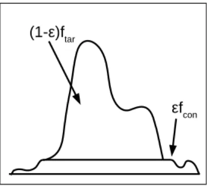
See Figure 3.1 for an example of a density satisfying this assumption. Because fcon must be uniform over the support of ftar a consequence of Assumption A is that
supp(ftar) has finite Lebesgue measure. LetVA be the contamination model
contain-ing all pairs of densities which satisfy Assumption A. Note that S
(ftar,fcon)∈VAftar is
exactly all densities whose support has finite Lebesgue measure, which includes all densities with compact support.
The uniformity assumption on fcon is a common “noninformative” assumption
on the contamination. Furthermore, this assumption is supported by connections to one-class classification. In that problem, only one class (corresponding to our ftar) is
observed for training, but the testing data is drawn from fobs and must be classified.
The dominant paradigm for nonparametric one-class classification is to estimate a level set offtar from the one observed training classTheiler and Cai (2003);Lanckriet
et al.(2003);Steinwart et al.(2005);Vert and Vert (2006);Sricharan and Hero(2011); Sch¨olkopf et al. (2001), and classify test data according to that level set. Yet level sets only yield optimal classifiers (i.e. likelihood ratio tests) under the uniformity
εfcon (1-ε)ftar
Figure 3.1: Density with contamination satisfying Assumption A
assumption on fcon, so that these methods are implicitly adopting this assumption.
Furthermore, a uniform contamination prior has been shown to optimize the worst-case detection rate among all choices for the unknown contamination densityEl-Yaniv and Nisenson (2007). Finally, our experiments demonstrate that the SPKDE works well in practice, even when Assumption A is significantly violated.
3.1.2 Decontamination Procedure
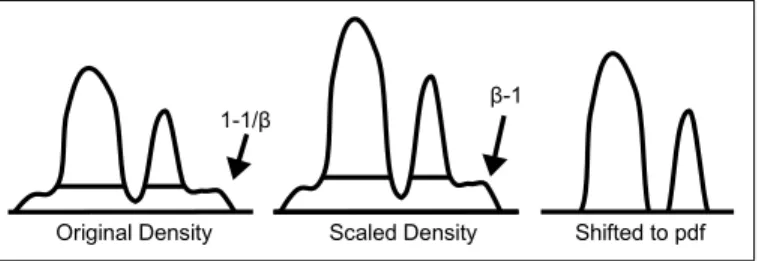
Under Assumption A ftar is present in fobs and its shape is left unmodified (up
to a multiplicative factor) by fcon. To recover ftar it is necessary to first scale fobs by
β = 1−1ε yielding
1
1−ε((1−ε)ftar+εfcon) =ftar+ ε
1−εfcon.
After scaling we would like to slice off 1−εεfcon from the bottom offtar+1−εεfcon. This
transform is achieved by max 0, ftar + ε 1−εfcon −α , (3.1)
whereα is set such that (3.1) is a pdf (which in this case is achieved withα =r1−εε). We will now show that this transform is well defined in a general sense. Let f be a
1-1/β
Original Density Scaled Density Shifted to pdf β-1
Figure 3.2: Infinite sample SPKDE transform. Arrows indicate the area under the line.
pdf and let
gβ,α = max{0, βf (·)−α}
where the max is defined pointwise. The following lemma shows that it is possible to slice off the bottom of any scaled pdf to get a transformed pdf and that the transformed pdf is unique.
Lemma III.2. For fixed β >1 there exists a unique α0 >0 such that kgβ,α0k
L1 = 1. Figure 3.2 demonstrates this transformation applied to a pdf. We define the following transform RA
ε : D → D where RAε(f) = max
1
1−εf(·)−α,0 where α is
such that RA
ε(f) is a pdf. The remaining mathematical proofs for this chapter are
deferred to Appendix A.
Proposition III.3. RAε decontaminates VA.
The proof of this proposition is an intermediate step for the proof for Theorem III.8. For any two subsets ofV,V0 ⊂D×D,R
εdecontaminatesV andV0 iffRε
decon-taminates VS
V0. Because of this, every decontaminating transform has a maximal set which it can decontaminate. Assumption A is both sufficient and necessary for decontamination by RA
ε, i.e. the set VA is maximal.
Proposition III.4. Let{(q, q0)} ∈ D×D and(q, q0)∈ V/
A. RεAcannot decontaminate
3.1.3 Other Possible Contamination Models
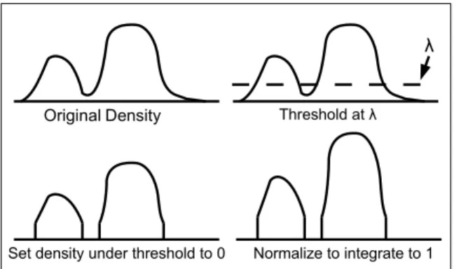
The model described previously is just one of many possible models. An obvious approach to robust kernel density estimation is to use an anomaly detection algorithm and construct the KDE using only non-anomalous samples. We will investigate this model under a couple of anomaly detection schemes and describe their properties.
One of the most common methods for anomaly detection is the level set method. For a probability measure µ this method attempts to find the set S with smallest Lebesgue measure such that µ(S) is above some threshold, t, and declares samples outside of that set as being anomalous. For a density f this is equivalent to finding λ such that R{x|f(x)≥λ}f(y)dy = t and declaring samples were f(X) < λ as being anomalous. Let X1, . . . , Xn be iid samples from fobs. Using the level set method for
a robust KDE, we would construct a density fbobs which is an estimate of fobs. Next
we would select some threshold λ > 0 and declare a sample, Xi, as being
anoma-lous if fbobs(Xi) < λ. Finally we would construct a KDE using the non-anomalous samples. Let χ{·} be the indicator function. Applying this method in the infinite
sample situation, i.e. fbobs = fobs, would cause our non-anomalous samples to come from the density p(x) = fobs(x)χ{τfobs(x)>λ} where τ = R χ{f(y)>λ}f(y)dy. See Figure
3.3. Perfect recovery of ftar using this method requires εfcon(x) ≤ftar(x) (1−ε) for
allx and that fcon and ftar have disjoint supports. The first assumption means that
this density estimator can only recover ftar if it has a drop off on the boundary of
its support, whereas Assumption A only requires that ftar have finite support. See
the last diagram in Figure 3.3. Although these assumptions may be reasonable in certain situations, we find them less palatable than Assumption A. We also evaluate this approach experimentally later and find that it performs poorly.
Another approach based on anomaly detection would be to find the connected components of fobs and declare those that are, in some sense, small as being
λ
OriginalDensity Threshold at λ
Set density under threshold to 0 Normalize to integrate to 1
Figure 3.3: Infinite sample version of the level set rejection KDE
which has a small mode. Unfortunately this approach also assumes thatftar andfcon
have disjoint supports. There are also computational issues with this anomaly detec-tion scheme; finding connected components, finding modes, and numerical integradetec-tion are computationally difficult.
To some degree, RA
ε actually achieves the objectives of the previous two robust
KDEs. For the first model, the RA
ε does indeed set those regions of the pdf that are
below some threshold to zero. For the second, if the magnitude of the level at which we choose to slice off the bottom of the contaminated density is larger than the mode of the anomalous component then the anomalous component will be eliminated.
3.2
Scaled Projection Kernel Density Estimator
Here we consider approximating RA
ε in a finite sample situation. Let f ∈L2 Rd
be a pdf and X1, . . . , Xn be iid samples from f. Let kσ(x, x0) be a radial smoothing
kernel with bandwidth σ such that kσ(x, x0) = σ−dq(kx−x0k2/σ), where q(k·k2)∈
L2
Rd and is a pdf. The classic kernel density estimator is:
¯ fσn:= 1 n n X 1 kσ(·, Xi).
we will scale our density by β >1 rather than 1
1−ε. For a density f define
Qβ(f),max{βf(·)−α,0},
where α = α(β) is set such that the RHS is a pdf. β can be used to tune robust-ness with larger β corresponding to more robustness (setting β to all the following transforms simply yields the KDE). Given a KDE we would ideally like to apply Qβ directly and search over α until max
βf¯n
σ (·)−α,0 integrates to 1. Such an
estimate requires multidimensional numerical integration and is not computationally tractable. The SPKDE is an alternative approach that always yields a density and manifests the transformed density in its asymptotic limit.
We now introduce the construction of the SPKDE. Let Dn
σ be the convex hull
of kσ(·, X1), . . . , kσ(·, Xn) (the space of weighted kernel density estimators). The
SPKDE is defined as fσ,βn := arg min g∈Dn σ βf¯σn−g L2,
which is guaranteed to have a unique minimizer since Dn
σ is closed and convex and
we are projecting in a Hilbert space (Bauschke and Combettes (2011) Theorem 3.14). If we represent fn σ,β in the form fσ,βn = n X 1 aikσ(·, Xi),
then the minimization problem is a quadratic program over the vector a = [a1, . . . , an]
T