Documents
de travail
Faculté des sciences économiques et de gestion
Pôle européen de gestion et d'économie (PEGE) 61 avenue de la Forêt Noire F-67085 Strasbourg Cedex Secétariat du BETA Géraldine Manderscheidt Tél. : (33) 03 90 24 20 69
«
External constraint and financial crises with
balance sheet effects
»
Auteurs Meixing Dai
Document de Travail n° 2009 - 02
External constraint and financial crises with balance sheet effects
Meixing DAI*
BETA-Theme, University Louis Pasteur (Strasbourg 1), France
Abstract: This paper examines a model of financial and exchange crises with balance-sheet
effects by explicitly taking account of wealth accumulation and external equilibrium condition. We have found that, in a general equilibrium analysis, there are two stationary equilibria. Since foreign debt is always zero at these equilibria, financial crises in emerging market economies cannot be interpreted as jumps between equilibria but between trajectories leading to one equilibrium or another one. The mechanisms of financial crises due to monsoon or spill-over effects are also analysed in this framework.
Keywords: Financial crisis, exchange crisis, balance sheet effect, external solvency
constraint.
JEL Classification: F31, F32, F41.
________________________________________ * Corresponding address:
Meixing DAI, University of Strasbourg, BETA-Theme, 61, avenue de la Forêt Noire – 67085 Strasbourg Cedex – France. Phone: (+33) 03 90 24 21 31; Fax: (+33) 03 90 24 20 71, e-mail: dai@cournot.u-strasbg.fr
1. Introduction
In the aftermath of 1997 Asian financial crisis, there was much controversy among macroeconomic researchers about its origin and nature. A decade later, economists have learned much about the relation between financial and exchange crises. Two generations of currency crisis models have been developed before the 1997 Asian turmoil and are pertinent in explaining other particular crisis in the 1990s. The first focused on budgetary deficits and the effect of its continuing monetary financing (Krugman, 1979; Flood and Garber, 1984). The second (Obstfeld, 1994; Sachs et al., 1996), explained the crisis as the result of a conflict between a nominal exchange rate peg and the desire of pursuing an expansionary monetary policy, leading to the existence of multiple equilibria.
In the major crisis countries of Asia, however, neither of these stories has much relevance. In terms of conventional fiscal measures, the governments of the distressed economies were in quite good shape at the beginning of 1997. While growth had slowed and some signs of excess capacity appeared in 1996, none of them faced the kind of clear trade-off between employment and exchange rate stability.
The third-generation models of currency crisis were then developed in order to answer the particular questions raised during this Asian crisis. Many of these models have in common the idea that the crisis should be seen as a result of a shock that is amplified by what Bernanke et al. (1999) have called a financial accelerator mechanism. The basic story is similar: Since firms’ assets and liabilities are denominated in domestic and foreign currency respectively, real currency depreciation can have a large effect on output if it affects the credit access of some subset of agents; moreover this effect on output may in turn affect the exchange rate, further amplifying the shock and causing it to persist. Most have argued that the core of the problem lies in the banking system. In Corsetti, Pesenti, and Roubini (1999), moral-hazard-driven lending could have provided a sort of hidden subsidy to investment, which collapsed when visible losses led governments to withdraw their implicit guarantees. Considering the Asian crisis as a problem of international financial fragility and liquidity, Chang and Velasco
(2001)1 suggest that currency crises are the by-product of a bank run. The later is modelled a
la Diamond and Dybvig (1983) and hence as a self-fulfilling loss of confidence that forces financial intermediaries to liquidate their investments prematurely. Krugman (1999) has sketched the transfer problem as another way of explaining the Asian crisis: foreign currency
1 The model of Chang and Velasco (2001) is not strictly a financial accelerator model. In fact, the effect on the
debts and firms’ leveraged financing make the domestic economy fragile and prone to crisis. In these models, there are multiple equilibria with the crisis brought on by a pure shift in expectations, leading to possible jump from high investment equilibrium to one with low or zero investment.
Meanwhile, in some models which introduce also balance sheet effects and leverage constraint, there is an adverse real shock that gets amplified. Aghion et al. (2001, 2004a) model a two-period multiple equilibrium economy in which the presence of sticky prices and foreign currency liabilities are part of a story of endogenous currency crises. In Mendoza (2002), a mismatch between the denomination of debt and income exacerbates financial crises in emerging markets. In Kim and Lee (2002), firms are motivated to over-invest because of government subsidies and are vulnerable to adverse shocks which increase rapidly the expected loan-to-collateral value ratio. In Aghion et al. (2004b), firms face credit constraints with the constraint being tighter at lower level of financial development. A basic implication of the model is that economies at an intermediate level of financial development are more unstable than either very developed or very underdeveloped economies. This is true both in the sense that temporary shocks have large and persistent effects and that these economies can exhibit cycles. In a small open economy model with sticky price and balance sheet effects, Cook (2004), shows that a monetary policy induced devaluation leads to a persistent contraction in output.
However, in modelling Asian financial crisis as jump from high investment equilibrium to low (or zero) investment equilibrium, one fails to take account of the characteristics of an emerging market economy and hence to explain the following recovery. In fact, the persistent
contractionary effects of devaluation are not found before and after the 1997 Asian crisis.2 For
example, South Korea saw its GDP growth rebounding from − 6.7 percent in 1998 to +10.9
percent in 1999. However, after currency devaluation, the level of GDP can remain
permanently below its initial trend,3 suggesting that the shocks underlying a currency crisis
are persistent (Hong and Tornell, 2005).
2 Empirically, Upadhyaya and Upadhyaya (1999) find that, with few exceptions, currency devaluation in Asian
countries fails to make any effect on output over any length of time - short run, intermediate run, or long run. Kim and Ying (2007), using the pre-1997 crisis data and the trade-weighted exchange rate, find no evidence of contractionary devaluations. In fact, currency devaluation appears strongly expansionary in several countries. But their exercise suggests also that the crisis period was indeed different.
3 This can also be explained by the shift, induced by violent shocks, in the behaviours of international lenders as
Moreover, most of these models focusing on balance sheet effects do not give enough attention to the rise of international interest rate. Kwack (2000) shows, with panel data on seven countries in Asia—Indonesia, Korea, Malaysia, Philippines, Singapore, Taiwan, and Thailand - for the 1995 through 1997 period, that the 3-month LIBOR interest rate and nonperforming loan ratios of banks are found to be the major determinants of the Asian financial crisis. The corporate leverage ratio also plays an important role since it explains the nonperforming loan ratios.
In this paper, we extend the model of Krugman (1999), in what follows Krugman, in taking account of wealth accumulation and external equilibrium condition. In analysing the dynamics of the economy, we find that a financial crisis can be considered as a jump from an
unstable trajectory to a stable (or unstable) trajectory among many others. In effect, emerging
market economies are in a process of capital and wealth accumulation so that the state where a crisis starts is necessarily a temporary equilibrium which, affected by some adverse shocks (such as a rise in foreign interest rate) or contagious financial crisis in neighbour countries, becomes a disequilibrium violating some basic financial constraints. Preventive devaluation as suggested by Miller (1998) is pertinent in avoiding excessive increase in foreign currency debt and subsequent financial crisis. The durable contractionary effects of devaluation can not appear in a dynamic analysis of emerging market model except when foreign currency debt is long term or/and too high.
In the section 2, we present the model that leads to a reduced dynamic system of investment and foreign debt. In the section after, we describe the steady state and the static and dynamic properties of multiple equilibria. In the section 4, we discuss factors which could be at the origin of financial fragility and crisis. The dilemma of stabilization under nominal exchange rate peg and some policy implications are respectively discussed in the sections 5
and 6. We conclude in the section 7.
2. The model
We extend the small open-economy model of Krugman, which does not include the money, to a multi-period model.
2.1. Basic equations
The small open economy model is described by the following equations:
α α − = = ( , ) 1 t t t t t G K L K L y , with Kt =It−1ptμ−1pt−μ and 0<α <1, (1)
X p y I X p C I yt =(1−μ) t +(1−μ) t + t =(1−μ) t +(1−α)(1−μ) t + t , (2) X I y pt = t[1−(1−α)(1−μ)]−(1−μ) t , (3) t t W I ≤(1+λ) , (4) ) , ( 1+rt =Gk Kt Lt , (5) * 1 1 ) 1 ( t t t t r p p r ≥ + + + , (6) 0 ≥ t I , (7) 1 * 1 1 1) (1 ) 1 ( + − − − + − − − = t t t t t t t y r D p r F W α , (8) t t t t t pF I W D + = − , (9) ). ( ) ( ) ( ) ( 1 1 1 * 1 1 1 1 1 * 1 1 − − − − − − − − − − − + − + − − ) − (1 − − = − + − + − − − − = t t t t t t t t t t t t t t t t t t t t t t t t t t ee F F p D D F p r D r y I X p F F p D D F p r D r C I X p B μ α μ μ μ (10)
with yt denotes the output, Kt the stock of physical capital, Lt the labour, It the investment,
t
C the consumption, pt thereal exchange rate (or the relative price of foreign goods), Xt the
exportations, Wt the net wealth of domestic entrepreneurs, Dt the domestic currency
denominated debt, Ft the foreign currency denominated debt, rt the domestic real interest
rate and *
t
r the foreign real interest rate. Some variables such as yt, Kt, It, Ct, Wt and Dt
are measured in terms of domestic goods while others, i.e. Xt and Ft, are in terms of foreign
goods. The time index “t” indicates that they are flux variable (yt, Lt, It and Ct) or prices
(pt, rt and rt*) of the current period, or stock variables at the end of the current period (Wt,
t
F and Dt) or of the last period (Kt).
Equation (1) represents the production function, assumed to be Cobb-Douglas, of the small open economy that produces a single good each period using capital and labour. Capital is created through investment and it is assumed that it lasts only one period, so that this period’s capital is equal to last period’s investment. This assumption allows putting aside Diamond-Dybvig-type concerns over maturity mismatch between capital and foreign debt.
According to Krugman, because a share μ of investment falls on foreign goods, the price
period in terms of domestic goods of current period is therefore deflated by a price index
μ μ
t
t p
p−−1 . In terms of modelling, it is equivalent to define Kt =It−1ptμ−1pt−μ.4
Equation (2) describes the market clearing condition for domestic goods. The functions of demand for consumption and investment are derived under the simple assumption that the residents of this economy are divided into two distinct classes. Workers, who receive a share
α
−
1 of domestic income, lack access to the capital market and therefore spend all their
income within each period. Entrepreneurs, who are assumed to be single-mindedly engaged in wealth accumulation, saving and investing all their income, create and own domestic capital until they have exhausted domestic investment opportunities. After that, they will spend their
surplus of their revenue over investment.5 The domestic and foreign goods, with a unitary
elasticity of substitution, are not perfect substitutes. A share 1−μ of both consumption and
investment is spent on domestic goods, μ on imports. The rest of the world is large and
spends a negligible fraction of its income on domestic goods. We assume, following
Krugman, that the value of domestic exports in terms of foreign goods is fixed with Xt =X ,
i.e. the foreign elasticity of substitution is also unitary.
From equation (2), the domestic real exchange rate is expressed as in equation (3). According to the later, the higher is investment, the lower the real exchange rate. The relationship between real exchange rate and investment is complicated by the presence of price index in the production function as indicated in equation (5).
As shown by inequality (4), the ability of domestic entrepreneurs to invest is limited by their wealth in the way of Bernanke et al. (1999). Lenders impose a limit on leverage, justified by microeconomic and financial motives such as risk of insolvability and asymmetric
information. Hence, entrepreneurs can borrow at most (1+λ)times their initial wealth.
Equation (5) shows that the return of domestic investment is determined by the marginal productivity of capital.
4
Krugman (1999) writes Kt=It−1p−μ, which represents a special case of the present model. In fact, Krugman
makes a partial equilibrium analysis of his model in adopting an implicit assumption, i.e. pt−1=1. 5
We introduce this assumption to close the small open-economy model. Otherwise, these entrepreneurs can accumulate an infinite amount of wealth. This assumption might not be plausible one for describing some emerging economies having sufficiently accumulated capital. As illustrated by recent international developments of South Korean firms, ambitious and innovative entrepreneurs might be tempted to invest on international financial market and in industrial projects in other countries. For other manners of closing the model, see Schmitt-Grohé and Uribe (2003).
According to inequality (6), entrepreneurs will not borrow beyond the point at which the real return on domestic investment, determined by equation (5), equals that on foreign investment. It is similar to uncovered interest rates parity (UIRP), which compares the return that can be achieved with domestic capital (by converting a unity of foreign goods into
domestic goods at the real exchange rate pt, then converting the next-period return back into
foreign goods at pt+1) and the rate of return of foreign asset rt*.
Equation (7) imposes that investment cannot be negative.
Entrepreneurs own a wealth which is defined by equation (8). They hold all domestic
capital and receive a share α of domestic revenue that will not be spent for consumption. The
income accruing to capital within the current period (αyt) also represents the value of
domestic capital since it lasts only one period. At aggregate level, they owe debt to international lenders with the “currency composition” of debt taken as a given.
Equation (9) describes the evolution of foreign debt contracted by domestic entrepreneurs. All investment not financed by their wealth is financed by foreign debt. In other words, it represents the balance-sheet constraint of these entrepreneurs.
Equation (10) is the external equilibrium condition or the balance of payments, which is equivalent to the combination of equations (2), (8) and (9) under flexible exchange rate
regime where the balance of payments exhibits neither deficit nor surplus, i.e. Bee=0. Under
fixed exchange rate regime, this equivalence is valid only at steady state since otherwise, Bee
can be positive, null or negative.
The last two equations represent the logic extension of Krugman’s model. They are important to our understanding of the underlying features of a crisis prone economy.
In the following, we assume for simplicity that the flexibility on the labour market will
ensure full employment and the supply of labour is normalized to unity so that Lt =1 ,∀t.
2.2 The behaviour of risk neutral entrepreneurs and iso-wealth curve
Risk neutral entrepreneurs maximise their wealth in period t+1 in solving the following program: t t t t t t t F D It t t W y r D p r F ) 1 ( ) 1 ( max 1 1 1 * , +1, +1, + =α + − + − + + , s.c. yt+1=(It ptμpt−+μ1)α, t t W I ≤(1+λ) ,
Dt + ptFt =It −Wt.
The Lagrangian of the above program can be written as:
Λ= (It pt pt 1) −(1+rt)Dt −pt+1(1+rt*)Ft − [It−(1+ )Wt]− (Dt +ptFt −It +Wt) −
+ ϕ λ γ
α μ μ α ,
where ϕ and γ are Lagrangian multipliers associated with leverage and balance-sheet
constraint respectively.
First-order conditions (FOC) for entrepreneurs’ wealth maximisation are: 0 1 1 2 − + = = ∂ Λ ∂ − + − ϕ γ α α αμ αμ t t t t p p I I , (11) , 0 ) 1 ( + − = − = ∂ Λ ∂ γ t t r D (12) . 0 ) 1 ( * 1 + − = − = ∂ Λ ∂ + t t t t p r p F γ (13)
FOC (12) and (13) imply that the UIRP is verified, i.e. t
t t
t r r p
p+1(1+ *)=(1+ ) . (14)
Using FOC (12) to find the value of γ and insert it into FOC (11) allows discussing
entrepreneurs’ decision relative to leveraged financing. If 2 1 −1 −(1+ )= >0
+ − ϕ α α αμ αμ t t t t p p r I ,
the leverage constraint (4) is binding. In other words, when the marginal rate of return of domestic investment is superior to the cost of financing additional investment, entrepreneurs find it advantageous to invest in borrowing from abroad the maximal amount allowed by the
leverage constraint. If 2 1 −1 −(1+ )≤0 + − t t t t p p r Iα αμ αμ
α , the constraint will not be binding and
entrepreneurs will borrow less than that is authorised by the leverage multiplier.
The parts of debt, denominated in domestic and foreign currency (or goods) respectively, cannot be determined without taking a more sophisticated approach of the behaviours of entrepreneurs and foreign banks under uncertainty and asymmetric information. For simplicity, we assume that they have a fixed ratio
ν = = − − 1 1 t t t t D F D F . (15)
This ratio can be the same for every period or be modified arbitrarily to examine the effect of its variation on economic equilibrium. In the following, current domestic-currency
denominated foreign debt Dt is simply named “foreign debt” even though the “total foreign
Foreign banks would pay attention to the wealth left to entrepreneur after the payment of principal and interests. If this financial indicator is zero or negative, no bank will lend to these entrepreneurs. Using equation (8) and taking account of equations (1), (14) and (15), we obtain: 1 * 1 1 1 1 (1 − ) − − − − − ⎥ + ⎦ ⎤ ⎢ ⎣ ⎡ + − = t t t t t t t t t pv r D p p p p I W α μ μ . (16)
If 0Wt < , when international lenders reduce their lending to zero, they will lose money. All
entrepreneurs will bankrupt and invest zero, i.e. the constraint (7) will be binding. For analytical purpose, we define an iso-wealth curve where entrepreneurs have the same level of
wealth independently of the level of foreign debt. For a given wealth W0, equation (16) can be
rewritten as: ) 1 ( ) 1 ( 1 *1 0 1 1 1 1 1 − − − − + − − − = + −+ t t t t t t t t r p vp W p p p I D μ μ α . (17)
Given the values of pt−1 and pt, there is an positive relation between investment and foreign
debt as shown in Figure 1, where on the horizontal axis is represented the foreign debt and on the vertical axis the investment. The iso-wealth curve shows the combinations of foreign debt and investment that ensure a constant wealth.
I Iso-wealth bis (W0') Iso-wealth (W0) C I0 O D D0
Figure 1: Iso-wealth curve.
A given combination of investment and foreign debt (I0,D0) can correspond to different
levels of entrepreneurs’ wealth according to the values of exogenous variables and parameters
According to equation (17), the curve Iso-wealth (Figure 1) will rotate counter-clockwise to a
position like the curve Iso-wealth bis corresponding to lower net wealth, W0', if there is:
- an increase in rt* that reduces entrepreneurs’ wealth.
- a decrease in X, since this implies according to equation (3) a depreciation of the real
exchange rate, decreasing the current value of domestic product but increasing the value of principal and interests on foreign debt.
- an increase in μ that, in increasing demand for foreign goods, implies a depreciation
of the real exchange rate and hence has similar effect as a decrease in X.
However, an increase in α has ambiguous effects on entrepreneurs’ wealth. It implies, on
the one hand, an increased revenue accrued to capitalists, and on the other hand, a depreciation of the real exchange rate (due to higher productivity of existing capital and hence higher output, and higher part of revenue that is exported for given investment) which increases thus the value of foreign debt when measured in domestic currency.
2.3. The reduced dynamic system
The model has nine endogenous variables, i.e. yt, Ct, It, Kt, rt, pt, Wt, Dt and Ft. It can be resolved in two steps. The first step consists to solve the reduced system of difference
equations describing the evolution of pt, It and Dt. In the second step, we can solve for Ft,
t
K , yt, Ct, rt and Wt, using market equilibrium condition, identities or behaviour equations.
Substituting yt defined by equation (1) into equation (3), we obtain:
X I p p I pt t 1 t 1 t [1 (1 α)(1 μ)] (1 μ) t αμ αμ α − − − − − = − − − . (18)
Given international interest rate, the highest level of investment, Iˆ , that is rational to
realise at stationary state, corresponds to the one that equalizes the marginal productivity of capital and the financial opportunity cost of investing. At steady state where
p p p
pt+1= t = t−1= , It−1=It =I , Dt =Dt−1=D and rt* =rt*−1=r*, taking account of
equations (1) and (14), equation (5) is rewritten as:
1+r*=αIα−1. (19)
Given *
α α − + = 1 1 *) 1 ( ˆ r I . (20)
At intermediate levels of investment inferior to Iˆ , the leverage constraint will be binding.
Since entrepreneurs are risk neutral and try to accumulate wealth as quickly as possible, investment dynamics is described by the binding leverage constraint (4). Using equations (1),
(8), (14) and (15) to eliminate Ft, Wt and rt, the difference equation for It is obtained as
follows: 1 * 1 1 1 1 1 (1 ) 1 ) 1 ( ) 1 ( − − − − − − − − + + + + = t t t t t t t t t p r D p vp p p I I λ α α αμ αμ λ . (21)
The dynamics of private foreign debt, which is equal to the country’s external debt in the
present model, can be described equivalently by equation (9) or equation (10) if Bee=0.
Using equation (9) and eliminating Ft, Wt and rt as before leads to:
1 * 1 1 1 1 1 (1 ) 1 ) 1 ( − − − − − − − + + + − = + t t t t t t t t t t t p r D p vp p p I I v p D α α αμ αμ . (22)
Equations (18) and (20)-(22) allow describing the dynamic behaviours of price, investment and foreign debt. They are non-linear difference equations and cannot be solved explicitly. However, the static and dynamic properties of this reduced system can be studied with the help of phase diagram.
3. Steady state
3.1. The steady state of the reduced dynamic system
The steady state equilibrium of the reduced dynamic system is defined by the vector (I,
p and D) which checks simultaneously the following equations, resulting from equations
(18) and (20)-(22) respectively: X I I p [1 (1 α)(1 μ)] (1 μ) α − − − − − = , (23) D r p v I I =(1+λ)α α −(1+λ)(1+ )(1+ *) , (24) D r p v I Iα − =(1+ ) * α , (25) α α − + = ≤ 1 1 *) 1 ( ˆ r I I . (26)
Given steady state level of investment, equation (23) determines the steady state real exchange rate. Equation (24) gives the combination of investment and foreign debt along the most rapid wealth accumulation path, limited by the condition (26). Equation (25) is the solvency constraint of entrepreneurs, which implies that the surplus of wealth over investment is equal to interest payments on foreign debt. Equation (25) can be substituted by its steady state equivalent resulting from equation (10), which is read as follows: in the absence of entry and exit of capital, the trade surplus must be equal to interest payments on foreign debt. Since the debt in this model is only foreign and contracted uniquely by entrepreneurs, their solvency constraint is then the same as the external solvency constraint of the economy.
3.2. Static properties of the reduced system
The system constituted of equations (23)-(25) can be decomposed into two sub-systems
that can be solved separately. Substituting p given by equation (23) into equations (24) and
(25) and rearranging the terms lead respectively to
) 1 ( } ) 1 ( )] 1 )( 1 ( 1 [ 1 { ) 1 ( ) 1 ( * r X I I v I I D inv + − − − − − + + − + = μ μ α λ α λ α α , (27) * } ) 1 ( )] 1 )( 1 ( 1 [ 1 { r X I I v I I D ee α μ μ α α α − − − − − + − = , (28) where inv D and ee
D denote, at different levels of investment, the highest steady state debt
compatible with leverage and external solvency constraint respectively. The effects of a variation of the real exchange rate on wealth and consequently on these two constraints are taken into account in these two equations. Equations (27) and (28) constitute a sub-system which can be solved to obtain the steady state values of investment and foreign debt.
For each value of inv
D , we can determine a “financeable” level of investment that would
occur if the leverage constraint (4) was binding. It determines via the effect of investment on the real exchange rate, and hence on balance sheets, how much credit could be extended to domestic firms at maximum. Since risk neutral entrepreneurs use maximally the leveraged financing, equation (27) represents also the set of combinations of foreign debt and optimal investment that is financed partially by entrepreneurs’ wealth and partially by foreign debt for all I <Iˆ.
I~ Id inv D I~id Iˆ A B ee D O D
Figure 2: Steady state and multiple equilibria.
According to equation (27), inv
D is positive for I∈]0,~I[ with ~I =
[
(1+λ)α]
1−1α and equalto zero for I =0 and I =I~. Equation (28) implies that
ee
D is positive for I∈]0,Id[ with
I
Id 1 ˆ
1 >
=α −α and equal to zero for I =0 and
d
I
I = . The relative position of
ee
D and
inv
D at steady state can be examined through their difference calculated using equations (27) and (28) as follows: } ) 1 ( )] 1 )( 1 ( 1 [ 1 { ) 1 )( 1 ( ) 1 ( ) 1 ( * * * X I I v r r I r I D D ee inv α μ μ λ λ λ α λ α α − − − − − + + + + + + + − = − . (29)
As the denominator of the fraction at the right hand of equation (29) is positive, it is easy to show: ⎪ ⎪ ⎩ ⎪⎪ ⎨ ⎧ < < = = > > − id id id ee inv I I I I I I D D ~ if , 0 ~ if , 0 ~ if , 0 , with α λ λ α λ − ⎥ ⎥ ⎦ ⎤ ⎢ ⎢ ⎣ ⎡ + + + = 1 1 * ) 1 ( ) 1 ( ~ r Iid . (30)
For I <I~id(respectively I =I~id or I >I~id), the level of foreign debt compatible with external equilibrium is superior (respectively equal or inferior) to the maximal foreign debt allowed by
the leverage constraint. The level of investment I~idcorresponding to the crossing point of
these two curves is not a steady state equilibrium since:
α α λ λ α λ α − − ⎥ ⎥ ⎦ ⎤ ⎢ ⎢ ⎣ ⎡ + + + = < + = 1 1 * 1 1 * (1 ) ) 1 ( ~ ) 1 ( ˆ r I r I id . (31)
Taking account of above discussion about the relative position of each curve, the curves
inv
D and
ee
D could be approximatively represented as in Figure 2.6
At high levels of I, the leverage constraint (4) will not bind. Instead, investment is
determined by equations (5) and (14) and consequently limited to Iˆ . According to condition
(26) as well as that Iˆ<I~,7 the dark thick curve representing the set of feasible combinations
of debt and investment is constituted of two parts, i.e. a horizontal part and a parabolic one
denoted by AB (i.e., I =Iˆ) and OB (i.e., the dark part on the curve
inv
D ) respectively. At
levels of investment inferior to Iˆ , it is optimal for risk neutral entrepreneurs to use fully the
leverage effect since this is the most rapid path of wealth accumulation. At Iˆ , entrepreneurs
may use a leverage inferior to (1+λ).
The positions of the curves
inv
D and
ee
D depend on the value of exogenous variables and
parameters such as X, r* μ, v and α while their respective intersection points with vertical
axis are unchanged. We remark that, whereas λ is a determinant of
inv
D , it does not affect
ee
D . These two curves are pulled to the left, if
- X decreases, implying a depreciation of the real exchange rate. That will increase the
value of foreign currency debt when measured in domestic currency.
- r* rises, increasing financial burden of foreign debt.
- μ increases, leading to similar effect as a decrease in X.
In effect, these changes in exogenous variables and parameters imply that the entrepreneurs’ wealth and the trade account surplus are reduced to levels that cannot anymore sustain the initial level of foreign debt and keep both leverage and external solvency constraints respected.
An increase in v also shifts these curves to the left. However, it exercises its effects
differently. In effect, it is equivalent to an increase of total foreign debt. To keep foreign debt at a constant level compatible with the leverage and external solvency constraints, both
domestic and foreign currency debt must be reduced. In the case of a decrease in λ, it limits
6 Some simple simulation exercises (using for example α =0.5, μ=0.5, =3
X , r*=0.05, v=2 and λ=2)
justify the form of curves drawn in this paper.
7
the foreign borrowing by entrepreneurs, but it does not affect the external solvency constraint which depends on the steady state trade surplus.
We remark that a variation of α has contradictory effects on the curves
inv
D and
ee
D . It
affects in an ambiguous manner the entrepreneurs’ wealth and hence the maximal amount of foreign debt which can be borrowed by them. It affects similarly the trade account and
therefore the level of foreign debt sustainable by the trade surplus.8 On the one hand, an
increase in α will raise the total revenue that can be distributed (due to positive effect on the
production) and the part of national revenue being distributed to entrepreneurs. That increases the surplus of entrepreneurs’ revenue over investment and thus their capability to repay principal and interests on foreign debt. In other words, it decreases relatively workers’ consumption and importations and increases the trade surplus necessary to pay interests on
foreign debt. On the other hand, an increase in α implies a depreciation of the real exchange
rate due to higher productivity of existing capital and hence larger output as well as larger part of output that can be exported. Due to this depreciation, the value of foreign currency debt increases in terms of domestic currency. Hence, total foreign debt becomes too high and must be reduced in order to be compatible with both leverage and external solvency constraints.
We admit that the foreign debt is non negative, i.e. D+ pF ≥0, ∀I . This condition
translates the assumptions according to which entrepreneurs have objective of attaining wealthy statute in exploiting as quick as possible all domestic investment opportunities; and once this statute is obtained, they will not seek to increase further their wealth by spending the
surplus of their revenue over the investment. Under the above condition, there are only two
stationary equilibria (Figure 2). One corresponds to the point O, where investment and foreign
debt are both zero. At this equilibrium, lenders do not believe that entrepreneurs have any collateral. Another equilibrium is the point A where foreign debt is zero and investment equal
8 Deriving
inv
D and
ee
D given respectively by equations (27) and (28) with respect to α leads to
) 1 ( } { ) 1 ( } ) 1 ( )] 1 )( 1 ( 1 [ ln { ] ) 1 [( ) ( ) ln 1 ( ) 1 ( * 2 r X I I I I I v X I I D inv + Π + + − + − − − − + − Π + + + ∂ ∂ = λ μ μ α α λ α λ α α α α α , * 2 } { } ) 1 ( )] 1 )( 1 ( 1 [ ln { ) ( ) ( ) ln 1 ( r X I I I I I v X I I D ee Π + − + − − − − − Π + + ∂ ∂ = α α α μ μ α α α α α ,
where Π=vIα[1−(1−α)(1−μ)]−v(1−μ)I, which is positive if we assume the real exchange rate is always positive (see equation (23)). As the numerator has a positive first term and a negative second term, the net effect
to Iˆ . At both equilibria, the equilibrium condition on domestic goods market and the external
equilibrium condition Bee=0 are realized.
In a two-period partial equilibrium analysis, Krugman has shown that there are three equilibria where investment is equal to financeable investment that depends on wealth and leveraged financing. Krugman outlines the following story about financial crisis: “a decline in capital inflows can adversely affect the balance sheets of domestic entrepreneurs, reducing their ability to borrow and hence further reducing capital inflows”. He imagines “a game in which lenders decide, in random order, how much credit to offer to successive domestic
entrepreneurs. The offer of credit depends on what the lenders think will be the value of the
borrower’s collateral. But because some debt is denominated in foreign goods, this value depends on the real exchange rate, and hence on the actual level of borrowing that takes place. A rational-expectations equilibrium of this game will be a set of self-confirming guesses— that is, the expected level of investment implicit in the credit offers must match the actual level of investment that takes place given those offers”.
A general equilibrium analysis of the steady state of the economy reveals that there are only two equilibria. The question is how the story of the financial crisis told above can be reinterpreted in terms of general equilibrium analysis. At aggregate level, the amount that entrepreneurs can borrow from international lenders to finance the investment depends on their wealth. The wealth of each individual entrepreneur depends on the level of such borrowing in the economy as a whole. Hence, we share the following basic point with Krugman: the borrowing of individual entrepreneur has a negative externality on the community, since the volume of capital inflow affects the terms of trade and hence the valuation of foreign-currency-denominated debt.
3.3. Dynamic properties of stationary equilibrium
The phase diagram represented in Figure 3 allows discussing the stability issue in an economy where entrepreneurs use foreign debt to finance their investment. At the right of the curve
ee
D , the external debt is too high in the sense that the trade surplus is not sufficient to
pay interests on existing debt and the foreign debt keeps increasing due to current account
deficit, vice versa. Under the line Iˆ and the left of the curve
inv
D , as the foreign debt is
and they can invest more and more. Above the line Iˆ the investment is too high and has a rate of return inferior to that offered by international financial market. Consequently, investment
must be reduced to increase the marginal rate of return of capital. Under the line Iˆ and at the
right of the curve
inv
D , the foreign debt is too high to satisfy the leverage constraint and the
entrepreneurs’ wealth will be insufficient to sustain the past level of investment. Therefore, investment must be reduced.
I I~ Id 6 inv D I~id 4 Iso-wealth (W0) 7 5 Iˆ A B 1 C ee D 2 3 O D
Figure 3: Multiple equilibria and phase diagram.
The equilibrium point A is stable. Meanwhile, the equilibrium point O is not stable since a small wealth is sufficient to start a wealth accumulating process which leads to higher and higher investment and foreign debt, leading the domestic economy finally to the equilibrium point A.
A more detailed discussion, in distinguishing seven areas in Figure 3, allows us to understand better the underlying dynamics of investment and foreign debt.
In area 1 (area ABO), bounded at the above by the line Iˆ and at the right by
inv
D , the foreign debt is inferior to the limit fixed by leverage constraint and is compatible with external solvency constraint. In this area, risk neutral entrepreneurs tend to invest in using at maximum the leveraged financing so that they can enrich themselves as quickly as possible. It implies that the quickest dynamic path, i.e. the segment OB of the curve
inv
D , will be chosen
by these entrepreneurs. They have the possibility to reduce progressively their foreign debt
and invest with their own financial resources once Iˆ is attained. While this path is possible, it
is extremely fragile and can lead to financial crisis when the domestic economy is facing adverse external shocks or international lenders turn pessimistic about the perspectives of the
domestic economy. Entrepreneurs with risk aversion will choose a wealth-accumulating path in the interior of the area ABO.
In area 2, delimited by the line Iˆ , the curve
ee
D and the curve OB, the investment is
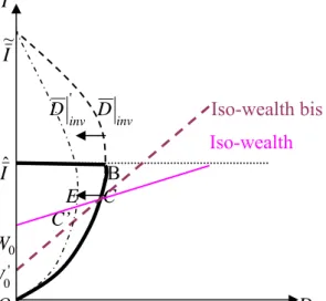
limited by the leverage constraint but not by the external solvency constraint. If the combination of investment and foreign debt happens to be in this area, entrepreneurs are constrained to reduce investment in order to reduce foreign debt. The temporary equilibrium that will realise after adjustment of international lending can be more or less favourable, depending on the confidence of international lenders placed on these entrepreneurs and the perspectives of the domestic economy. The adjustment imposed by international lenders may
not be coordinated. For a level of wealth W0, instead of reducing their lending to a level
corresponding to a point such as C, international lenders with herd behaviour could reduce
their lending to zero, diminishing hence the investment to a level equal to W0.9 A jump from a
situation of disequilibrium with high foreign debt to a temporary equilibrium without it becomes possible when the debt is short run. In other words, the foreign debt is a jumping variable (or non-predetermined) and can be adjusted freely.
In area 3, which is at the right of the curve
ee
D and under the line Iˆ, entrepreneurs have
high foreign debt, exceeding the limit imposed by the leverage constraint as well as that by external solvency constraint. If the foreign debt is not too high, a quick reaction of international lenders will allow them to recover totally or most of their lending with interests. If they wait, the situation could deteriorate and lead to their loss while all entrepreneurs bankrupt.
In area 4, above the line Iˆ and bordered at the left by the curve
inv
D for I >I~id and the curve
ee
D for I∈]Iˆ,~Iid[, the investment is higher than Iˆ and the foreign debt is higher than
the highest level compatible with both leverage and external solvency constraints. Rational
entrepreneurs will reduce their investment until Iˆ . The reaction of international lenders will
depend on the initial level of foreign debt as well as that of wealth.
In area5,between curves
inv
D and
ee
D with I∈]Iˆ,~Iid[, the investment is higher than Iˆ . The foreign debt is higher than the highest level compatible with the leverage constraint and
9
To the difference of Krugman (1999), not all firms will bankrupt and investment will not finally fall to zero in this general equilibrium analysis.
lower than that respecting the external solvency constraint. Rational entrepreneurs will reduce
their investment until Iˆ . If they do not make this decision, they will be constrained by foreign
lenders to reduce their investment after all. Since foreign debt is not excessively high and entrepreneurs’ wealth is large, a severe financial crisis is impossible.
In area 6, between curves
inv
D and
ee
D with I >I~id, the investment is higher than Iˆ
while the foreign debt is lower than the highest level compatible with the leverage constraint but higher than that respecting the long term external solvency constraint. Rational
entrepreneurs will reduce their investment until Iˆ as well as their debt. If they do not reduce
their investment, the foreign debt will increase due to unpaid interests and that will not be allowed by rational and well-informed international lenders who take account of the external equilibrium condition of the small country.
In area 7, delimited at the above by the curve
ee
D , ∀I∈]~Iid,Id[ and at the right by the curve
inv
D with I∈]Iˆ,~Iid[, the investment is higher than Iˆ . The foreign debt is lower than
the highest level compatible with both leverage and external solvency constraints. Entrepreneurs will reduce their investment and foreign debt until the equilibrium point A is attained.
In the areas 1 and 7, the behaviour of this model is relatively uninteresting in terms of crisis probability. In the area 1, the economy has a high rate of return on investment and may find that adjustment of its capital stock is delayed by not having leverage constraint binding. In the area 7, reducing orderly both investment and foreign debt is optimal and feasible. An outburst of financial crisis is improbable since the wealth is sufficiently high with regard to existing foreign debt. In these two cases, there will be nothing that resembles an Asian-style financial crisis as discussed in the literature.
The financial crisis in this model then cannot be explained by jumps between the multiple stationary equilibria due to self-fulfilling expectations. Meanwhile, they can be interpreted as jumps from a temporary equilibrium with high foreign debt to another one with less or no foreign debt, situated on two different dynamic trajectories. To make this possible, one can consider some factors that make foreign lenders panicking. In this respect, two channels of contagion, i.e. monsoonal effects and spill-over effects (Masson, 1999a, b), can be used here to explain a financial crisis. The monsoonal effects emanate from the global environment (in particular, from policies in industrial countries), and sweep over all emerging countries to a
raising thus the financial costs of investment for an indefinite horizon. Due to spill-over effects, crisis in one country may affect other emerging markets through the linkages operating through trade, economic activities or competitiveness. A typical example is a currency devaluation of a rival country in crisis, which reduces potentially the exportations of the domestic economy.
Due to the effects of contagion, an economy initially on a feasible accumulation path such as OB in Figure 3 may be found to be situated at the right of the curve
inv
D or at worst at the
right of the curve
ee
D as these curves shift to the left. For emerging economies that initially
offer high rate of return of capital, this situation can result from previous choices of entrepreneurs who underestimate the effects of exogenous shocks on macroeconomic and financial stability and the repercussion of these shocks on the rate of return of their own investment.
We remark that although the leveraged financing is assumed to have a rigid multiplierλ,
international lenders can choose to reduce drastically the debt to a level that they consider as safe for their principal and interest payments, in particular when the debt is short-run. Under a flexible exchange regime, a severe reduction of investment and foreign debt in a short time can take place when some shocks modify drastically and adversely the current and future real exchange rates and hence reduce entrepreneurs’ wealth to a dangerous low level.
Any temporary equilibrium along the line OB is submitted to the possibility that a loss of lenders’ confidence will be validated by financial collapse if these lenders change radically their behaviour. In normal time, domestic entrepreneurs could finance their investment in using at maximum the leveraged financing. But in bad time, panicking international lenders could reduce arbitrarily the leverage multiplier to level that they consider as safe. They would examine attentively if the exogenous shocks are sufficiently important so that the economy is going to collapse with investment and entrepreneurs’ wealth falling to zero. This scenario is possible only if investment and foreign debt are both jumping variables. If the investment is only amortised partially and the foreign debt is long term, the immediate collapse will be less severe and these two variables will be on a path of crawling crisis with less violence.
4. Factors at the origin of financial fragility and crisis
It is largely documented that Asian countries, which have been drawn into 1997 financial crisis, had a balance of payments characterized by large current account deficits compensated
by net inflow of foreign capital. In our model, this could correspond to a situation where ambitious entrepreneurs expand their investment using at maximum the leveraged financing along or near the line OB. That implies an increasing inflow of foreign capital.
Even the basic part of our model is the same as Krugman, the story that we will talk is quite different from his one. In fact, Krugman worked with three equilibria that are made possible in using a partial static equilibrium analysis. A financial crisis corresponds then to a jump from one equilibrium with high investment to another one with zero investment with all entrepreneurs bankrupt, given that an intermediate equilibrium is not stable.
In this paper, a general equilibrium analysis shows there are only two steady state equilibria. Consequently, a financial crisis is an inherent phenomenon of an emerging market economy that uses extensively foreign debt (foreign currency denominated or not) to finance its development. It is a jump from one trajectory of wealth-accumulating to another one with less investment and lower foreign debt when international lenders become pessimistic. When a more or less severe financial crisis takes place, not all entrepreneurs are bankrupt systematically. The collapse (or shift from one dynamic trajectory of high debt to another one with low or no debt) does not indicate that the previous investments were unsound. The problem is instead one of financial fragility in a dynamic context.
4.1. Factors at the origin of financial fragility
The financial fragility in this kind of model has nothing to do with the mismatch between short-term debt and long-term investments; nor does it appear to depend on foreign exchange reserves. Krugman has highlighted the difference between his story of financial fragility and that told by others (e.g. Chang and Velasco, 2001) by considering the conditions under which this fragility can occur — namely, when financeable investment responds more than one to actual level of investment. That leads him to consider the following factors as being able to make financial collapse: (i) High leverage; (ii) Low marginal propensity to import; (iii) Large foreign-currency debt relative to exports.
What is then the role of these factors in the present model? We examine in the following if they make the domestic economy more fragile and more likely to fall into financial crisis when facing adverse exogenous shocks or unfavourable change in international lenders’ opinion.
An increase in the leverage, i.e. higher λ, will shift the curve
inv
D to the right without
modifying the position of the curve
ee
D . Whatever is the value of λ, the curve
inv
D is
always at the left of the curve
ee
D in the space of (D, I) for I <Iˆ. But as the curve
inv
D is
closer to the curve
ee
D , ∀I <Iˆ, a temporary equilibrium point like B’ in Figure 4 is less
susceptible of keeping the confidence of international lenders than a point like B. In effect, if exogenous shocks come to shift the curve
ee
D to the left, it is more probable to find the point
B’ at the right of the new curve (not drawn in Figure 4) representing the external equilibrium condition. That corresponds to a situation where the external debt of the small economy is not sustainable given the economic and financial conditions.
I I~ inv D Id I~id Iso-wealth (W0) Iˆ A B B’ C ee D O D
Figure 4: High leverage and steady state equilibrium.
Low marginal propensity to import
A decrease in marginal propensity to import will shift the curves inv
D and
ee
D to the
right with the later being more sensible (Figure 5). Since a low marginal propensity to import leads domestic entrepreneurs to contract higher foreign debt, it will increase the fragility of the domestic economy and reduce its ability to resist adverse shocks.
I I~ d I inv D I~id Iso-wealth (W0) Iˆ A B B’ C ee D O D
Figure 5: Low marginal propensity to import and steady state equilibrium.
Large foreign-currency debt relative to exports
The ratio of foreign-currency debt relative to exports is a complex indicator which is not clearly discussed by Krugman. In terms of static comparatives, a large ratio of foreign-currency debt relative to exports can be due to multiple factors. Using equations (15), (23) and (27), the ratio can be written as:
) 1 ( } ) 1 ( )] 1 )( 1 ( 1 [ { ) 1 ( ] ) 1 [( } ) 1 ( )] 1 )( 1 ( 1 [ { * r I v I v X X I I I v I v X pvD X pF + − − − − − + + − + − − − − − = = μ μ α λ α λ μ μ α α α α . (32)
An increase in v, μ, λ and α as well as an decrease in r* and X could lead domestic
firms to contract a larger foreign currency debt, implying an increase in the ratio pFX .10 A
larger ratio pFX will make these firms more vulnerable to financial crisis. The ratio depends
also on the investment and hence the stage of economic development. It is to note that some
parameters or exogenous variables, such as λ, *
r and X , can vary adversely and brutally,
leading to financial crisis as discussed in the following.
4.2. Factors at the origin of a financial crisis
The factors discussed above explain the fragility of emerging market economy using foreign debt to finance its development. They matter because they make the circular loop
10 If
I is sufficiently high so that lnI >0, we have then
0 ) ( ] ln ) 1 ( ) 1 [( } ) 1 ( ln )] 1 )( 1 ( 1 [ { ] ) 1 [( ) ( > = + − − − − + − +Π + + + +Π ∂ X I I v I I vI I I I X X pF λαα α μ α α μ λ α λαα .
from past investment to real exchange rate to balance sheets to current investment more powerful. But they don’t explain why Asian financial crisis takes place. All afflicted Asian economies were peculiarly vulnerable to financial crisis due to high leverage and unusually high levels of debt denominated in foreign currency. These borrowings have placed them at
risk of financial collapse if the real exchange rate depreciated.Before discussing the impact of
a depreciation of the real exchange rate resulting from a devaluation of the domestic currency, we show that the factors that were present in Asian crisis can also generate a financial crisis
under floating exchange rate regime. Generally, the factors leading to financial fragility can
become factors at origins of financial crisis if they come to change adversely. Consider here some others not considered in the above discussion.
Foreign monetary policy
One important factor which is present previous to Asian financial crisis is the high 3-month Libor interest rate (Kwack, 2000). In effect, previous to the crisis, the Fed has adopted a restrictive stance for its monetary policy, inducing hence higher interest on international financial markets. This shock can affect considerably the temporary equilibrium based on
leveraged financing. According to equations (27) and (28), an increase in r* shifts the line Iˆ
to 'Iˆ , and the curves inv
D and
ee
D to the left (Figure 6).
I I~ d I inv D
Iso wealth bis (W0')
I~id Iso-wealth (W0) Iˆ A B 'Iˆ B’ ee D O D
Figure 6: An increase in foreign interest rate.
An increase in foreign interest rate reduces the foreign funds disposable for domestic entrepreneurs. Furthermore, this is unfavourable to their personal wealth for the following
the net wealth is sufficiently high at the initial temporary equilibrium, the following adjustment can place the economy on a trajectory such as the curve OB’. In the contrary, the foreign debt can jump to a low level if it is short term or follow a trajectory characterized by crawling financial crisis if it is long term.
Lender’s attitudes towards domestic entrepreneurs
In the present model, the leverage of investment over entrepreneurs’ wealth is considered as fixed. When a financial crisis hits other emerging economies, lenders may change their mind and hence reduce the leverage multiplier. In this case, the curve
inv
D shifts to the left,
while the curve ee
D stays unmoved (Figure 7).
A reduction in the leverage multiplier may translate an increased risk aversion or loss of confidence of international lenders on the future perspectives of the domestic economy or/and world economy. It is not sufficient to lead to the occurrence of a financial crisis except when their pessimistic expectations are realised. If entrepreneurs’ wealth is not influenced, investment and foreign debt will adjust orderly towards lower levels.
I I~ inv D Id I~id Iso-wealth Iˆ A B’ B ee D W0 O D
Figure 7: A decrease in the leverage multiplier.
Contagious financial crisis
A currency devaluation of a neighbour country that is competitor of the domestic county
on the international goods market reduces the latter’s exportations.11 That shifts the curves
11 We neglect the effect of neighbour country’s currency devaluation on the domestic price level. This can be
inv
D and
ee
D to the left and could make the initial temporary equilibrium with high
investment and high foreign debt unsustainable judging by the leverage constraint and/or external equilibrium condition. If the leverage constraint is not respected meanwhile external solvency constraint is respected, the panic of lenders may be not very severe since the reduction of liquidity in the domestic economy will not bankrupt all entrepreneurs. In effect, a reduction of exportations will impact negatively the entrepreneurs’ wealth since it implies a depreciation of the real exchange rate and hence increases the value of foreign currency debt measured in domestic currency. A surprise decrease in exportations would make some domestic entrepreneurs insolvent and could lead to a financial crisis. The severity of the crisis depends on initial wealth, leverage multiplier as well as amplitude of the fall in exportations.
Particularly, if the external solvency constraint is also violated, a deep crisis may materialize since the high level of debt may be backed by an insufficient level of wealth or even negative wealth. Consequently, the liquidation of all firms may not leave enough financial resources to pay all foreign debt and interests.
5. The dilemma of stabilization under nominal exchange rate peg
In the period before 1997, Asian countries have grown rapidly and liberalised their capital account as urged by the FMI while keeping nominal exchange rate peg. The peg of Asian monies to US dollar is an important characteristic that is not taken into account in the previous description of the model. Even the model does not include explicitly the money market to allow analysing monetary or exchange rate policies, we can however discuss the
effect of a fixed nominal exchange rate on economic equilibrium and dynamics. If domestic
and foreign inflation rates are equal, a fixed nominal exchange rate is equivalent to a fixed
real exchange rate12. The inflation rate is often higher in emerging economies, without
excluding the contrary, than in their developed counterparts due to abundant inflow of foreign capital and liquidity. If this is the case, a fixed nominal exchange rate implies regular
appreciation of the real exchange rate, i.e. a decrease in p relative to its value in previous
period.
Fixed real exchange rate
To avoid the risks of financial trauma due to foreign currency debt was a major reason why the IMF advised its Asian client countries to follow the much-criticized “IMF strategy” which consists to defend their currencies with high interest rates rather than simply letting them devaluate. Even though this model does not allow a direct analysis of monetary policy, we can get some insight at the nature and consequences of the IMF strategy by imagining that
the effect of that strategy is to hold the real exchange rate p constant even when the
willingness of international lenders to finance investment declines.
Consider the case where domestic and foreign inflation rates are equal and real exchange
rate is maintained fixed using nominal exchange rate peg. Since p is fixed, the natural
assumption to ensure the equilibrium on domestic goods market, as adopted by Krugman, is
that the output adjusts instead to the aggregate demand. Considering that p is exogenously
controlled as fixed, the steady state output will be determined by a sort of quasi-Keynesian multiplier process. Rearranging equation (2) gives:
α μ α μ I X p I y ≤ ) − )(1 − (1 − + ) − 1 = 1 ( . (33)
The realised output is inferior or equal to the production capacity, i.e. y≤Iα. Inserting the
value of y defined by equation (33) to substitute the distributed national revenue, which is
α
I under flexible exchange rate regime, in equations (24) and (25) yields:
] 1 )[ 1 )( 1 )( 1 ( ) 1 ( ] ( [ * −(1− )(1− ) + + + + + − ) − 1 = μ α λ α λ μ μ λα r p v X p I D inv , (34) * ) 1 ]( 1 [ vp r I X p D ee −(1− )(1− ) + − = μ α μ α . (35)
The slope of the curve
ee
D is clearly negative and that of the curve
inv D is positive if + < λα λα μ
1 . The equilibrium determined by equations (34) and (35) is unstable
13 as illustrated in Figure 8. This equilibrium would be disqualified as sustainable steady state
equilibrium if it is situated above the line Iˆ (not represented in Figure 8).
Above the line inv
D , the investment is high and the foreign debt is relatively low.
Entrepreneurs increase their investment and hence their wealth. At the right of the curve ee
D ,
13 The slope of the curve
inv
the trade surplus is not sufficient to pay interests on the foreign debt, consequently the foreign
debt will increase due to current account deficit. An increase in p induced by a devaluation
of the domestic currency will impact both curves as follows:
] 1 )[ 1 ( ) 1 )( 1 ( ] ( [ ) 1 ( * 2 + −(1− )(1− ) + + − ) − 1 − + = ∂ ∂ μ α λ μ μ λα α λ r p v v I X p D inv , (36) 0 ) 1 ]( 1 [ −(1− )(1− ) + 2 * > + = ∂ ∂ r p v v I X p D ee μ α μ α . (37)
The effects of an increase in p on
inv
D depends on the level of investment while that on
ee D is always positive. I ' inv D inv D B IA A IR R A’ ee D O D
Figure 8: Instability under fixed nominal and real exchange rates.
The level of investment for which an increase in p has no effect on the curve
inv D is defined using (36) as v X IR ] ( [ ) 1 ( μ μ λα α λ − ) − 1 + = . (38)
Using equations (34) and (35), the level of investment corresponding to initial equilibrium is defined as: μ λ μ μ λα α λ ) 1 ( ( ) 1 ( * * r r X p IA + + + ) − 1 + = . (39)
For the initial equilibrium A to situate at the right of the curve '
inv
D , it is necessary that
the investment corresponding to the rotation point of the curve
inv
D is inferior to its initial