UC Merced Electronic Theses and Dissertations
TitleLearning Spatial and Temporal Visual Enhancement
Permalink https://escholarship.org/uc/item/2cg6q5rc Author Lai, Wei-Sheng Publication Date 2019 Peer reviewed|Thesis/dissertation
eScholarship.org Powered by the California Digital Library
UNIVERSITY OF CALIFORNIA, MERCED
Learning Spatial and Temporal Visual Enhancement
A dissertation submitted in partial satisfaction of the requirements for the degree
Doctor of Philosophy in
Electrical Engineering and Computer Science by
Wei-Sheng Lai
Committee in charge:
Professor Ming-Hsuan Yang, Chair Professor Shawn Newsam
Professor Sungjin Im Professor Jia-Bin Huang
The dissertation of Wei-Sheng Lai is approved, and it is acceptable in quality and form for publication on microfilm and electronically:
Professor Shawn Newsam
Professor Sungjin Im
Professor Jia-Bin Huang
Professor Ming-Hsuan Yang Chair
University of California, Merced
2019
Signature Page . . . iii
Table of Contents . . . iv
List of Figures . . . vii
List of Tables . . . xii
Vita and Publications . . . xiv
Abstract . . . xvi
Chapter 1 Introduction . . . 1
1.1 Overview . . . 1
1.2 Organization . . . 2
Chapter 2 Literature Review . . . 4
2.1 Single Image Super-Resolution . . . 4
2.1.1 SR Using Internal Databases . . . 4
2.1.2 SR Using External Databases . . . 5
2.1.3 CNN-based SR . . . 5
2.1.4 Laplacian Pyramid . . . 6
2.1.5 Adversarial Training . . . 8
2.2 Video Temporal Consistency . . . 8
2.2.1 Task-Specific Approaches . . . 8 2.2.2 Task-Independent Approaches . . . 9 2.3 Video Stitching . . . 10 2.3.1 Image Stitching . . . 10 2.3.2 Video Stitching . . . 11 2.3.3 Pushbroom Panorama . . . 11
Chapter 3 Fast and Accurate Image Super-Resolution with Deep Laplacian Pyra-mid Networks . . . 12
3.1 Introduction . . . 12
3.2 Deep Laplacian Pyramid Network for SR . . . 16
3.2.1 Network Architecture . . . 16
3.2.2 Feature Embedding Sub-network . . . 17
3.2.3 Loss Function . . . 19
3.2.4 Multi-Scale Training . . . 21
3.2.5 Implementation and Training Details . . . 21
3.3 Discussions and Analysis . . . 22
3.3.1 Model Design . . . 22
3.3.2 Parameter Sharing . . . 25
3.3.3 Training Deeper Models . . . 26
3.3.4 Multi-Scale Training . . . 28
3.4 Experimental Results . . . 29
3.4.1 Comparisons with State-of-the-arts . . . 31
3.4.2 Execution Time . . . 34
3.4.3 Model Parameters . . . 34
3.4.4 Super-Resolving Real-World Photos . . . 37
3.4.5 Comparison to LAPGAN . . . 37
3.4.6 Adversarial Training . . . 39
3.4.7 Human Subject Study . . . 40
3.4.8 Limitations . . . 43
3.5 Conclusions . . . 44
Chapter 4 Learning Blind Video Temporal Consistency . . . 45
4.1 Introduction . . . 45
4.2 Learning Temporal Consistency . . . 48
4.2.1 Recurrent Network . . . 48
4.2.2 Loss Functions . . . 48
4.2.3 Image Transformation Network . . . 51
4.2.4 Implementation Details . . . 52
4.3 Experimental Results . . . 53
4.3.1 Datasets . . . 53
4.3.2 Applications . . . 54
4.3.3 Evaluation Metrics . . . 55
4.3.4 Analysis and Discussions . . . 56
4.3.5 Comparison with State-of-the-arts . . . 61
4.3.6 Subjective Evaluation . . . 61
4.3.7 Execution Time . . . 65
4.3.8 Limitations and Discussion . . . 65
4.4 Conclusions . . . 67
Chapter 5 Learning to Stitch Videos for Structured Camera Arrays . . . 68
5.1 Introduction . . . 68
5.2 Stitching as Spatial Interpolation . . . 72
5.2.1 Problem Setup . . . 72
5.2.2 Formulation . . . 73
5.2.3 Fast Pushbroom Interpolation Layer . . . 76
5.2.4 Training Pushbroom Stitching Network . . . 77
5.3 Experimental Results . . . 80
5.3.1 Model Analysis . . . 80
5.3.2 Comparisons with Existing Methods . . . 84
5.3.3 Limitations and Discussion . . . 87
5.4 Conclusions . . . 90
6.2 Future Work . . . 92 6.2.1 Practical Applications of Low-Level Vision . . . 92 6.2.2 Semi-Supervised Learning and Domain Adaptation . . . 93 6.2.3 Learning-Based Computational Photography . . . 93 Bibliography . . . 95
LIST OF FIGURES
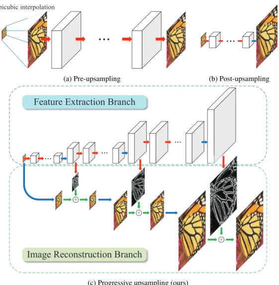
Figure 3.1: Comparisons of upsampling strategies in CNN-based SR algo-rithms. Red arrows indicate convolutional layers. Blue arrows in-dicate transposed convolutions (upsampling), and green arrows denote element-wise addition operators. (a) Pre-upsampling based approaches (e.g., SRCNN [24], VDSR [57], DRCN [58], DRRN [103]) typically use the bicubic interpolation to upscale LR input images to the tar-get spatial resolution before applying deep networks for prediction and reconstruction. (b) Post-upsampling based methods directly extract features from LR input images and use sub-pixel convolution [98] or transposed convolution [25] for upsampling. (c) Progressive upsam-pling approach using the proposed Laplacian pyramid network recon-structs HR images in a coarse-to-fine manner. . . 14 Figure 3.2: Detailed network architecture of the proposed LapSRN. At each
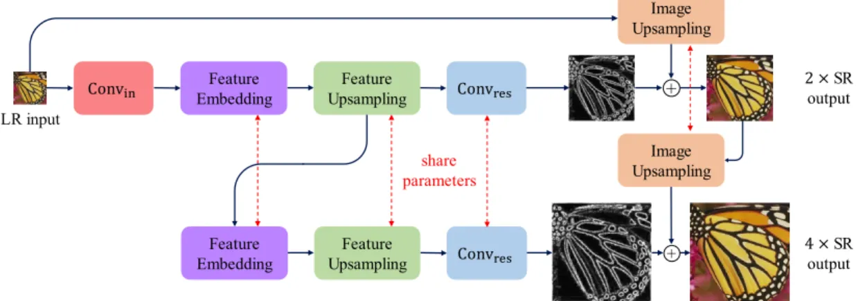
pyramid level, our model consists of a feature embedding sub-network for extracting non-linear features, transposed convolutional layers for upsampling feature maps and images, and a convolutional layer for predicting the sub-band residuals. As the network structure at each level is highly similar, we share the weights of those components across pyramid levels to reduce the number of network parameters. . . 16 Figure 3.3: Local residual learning. We explore three different ways of local skip
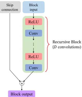
connection in the feature embedding sub-network for training deeper models. . . 19 Figure 3.4: Structure of our recursive block. There areDconvolutional layers
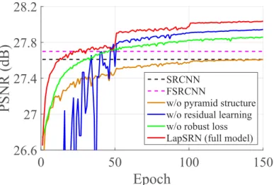
in a recursive block. The weights of convolutional layers are distinct within the block but shared among all recursive blocks. . . 20 Figure 3.5: Convergence analysis. We analyze the contributions of the
pyra-mid structures, loss functions, and global residual learning by replac-ing each component with the one used in existreplac-ing methods. Our full model converges faster and achieves better performance. . . 23 Figure 3.6: Contribution of different components in LapSRN. (a) Ground truth
HR image (b) without pyramid structure (c) without global residual learning (d) without robust loss (e) full model (f) HR patch. . . 24 Figure 3.7: Contribution of multi-scale supervision (M.S.). The multi-scale
su-pervision guides the network training to progressively reconstruct the HR images and help reduce the spatial aliasing artifacts. . . 24 Figure 3.8: Comparisons of local residual learning. We train our
LapSRN-D5R5 model with three different local residual learning methods as described in Section 3.2.2 and evaluate on the SET5 for4×SR. . . 27 Figure 3.9: PSNR versus network depth. We test the proposed model with
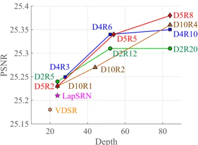
dif-ferentDandRon the URBAN100 dataset for4×SR. . . 29
Figure 3.10: Visual comparison of multi-scale training. . . 30
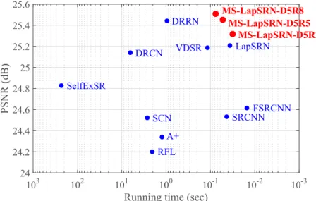
Figure 3.12: Runtime versus performance. The results are evaluated on the UR -BAN100 dataset for4×SR. The proposed MS-LapSRN strides a bal-ance between reconstruction accuracy and execution time. . . 36 Figure 3.13: Trade-off between runtime and upsampling scales. We fix the size
of input images to 128×128 and perform 2×, 4× and 8× SR with the SRCNN [24], FSRCNN [25], VDSR [57] and three variations of MS-LapSRN, respectively. . . 36 Figure 3.14: Number of network parameters versus performance. The results
are evaluated on the URBAN100 dataset for4×SR. The proposed
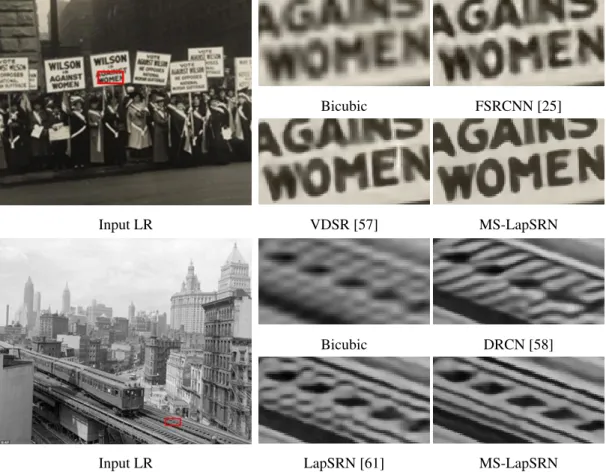
MS-LapSRN strides a balance between reconstruction accuracy and execu-tion time. . . 37 Figure 3.15: Comparison of real-world photos for 4×SR.The ground truth HR
images and the blur kernels are not available in these cases. On the top image, our method super-resolves the letter “W” accurately while VDSR incorrectly connects the stroke with the letter “O”. On the bot-tom image, our method reconstructs the rails without the artifacts. . . . 38 Figure 3.16: Visual comparison for adversarial training. We compare the results
trained with and without the adversarial training on4×SR. . . 39 Figure 3.17: Interface for our human subject study. Human subjects can switch
back and forth between two given images (results from two different super-resolution algorithms) to see the differences. . . 41 Figure 3.18: Analysis on human subject study. Our MS-LapSRN is preferred
by75%and80%of users on the BSDS100 and URBAN100 datasets, respectively. The error bars show the95%confidence interval. . . 42 Figure 3.19: Limitation. A failure case for 8× SR. Our method is not able to
hallucinate details if the LR input image does not consist of sufficient amount of structure. . . 43 Figure 4.1: Applications of the proposed method. Our algorithm takes
per-frame processed videos with serious temporal flickering as inputs (lower-left) and generates temporally stable videos (upper-right) while main-taining perceptual similarity to the processed frames. Our method is blind to the specific image processing algorithm applied to input videos and runs a high frame-rates. This figure contains animated videos, which are best viewed using Adobe Acrobat. . . 46 Figure 4.2: Overview of the proposed method.We train an image transformation
network that takesIt−1, It, Ot−1 and processed framePtas inputs and
generates the output frameOtwhich is temporally consistent with the
output frame at the previous time step Ot−1. The output Ot at the
current time step then becomes the input at the next time step. We train the image transformation network with the VGG perceptual loss and the short-term and long-term temporal losses. . . 49
Figure 4.3: Temporal losses. We adopt the short-term temporal loss on neighbor frames and long-term temporal loss between the first and all the output frames. . . 50 Figure 4.4: Architecture of our image transformation network. We split the
input into two streams to avoid transferring low-level information from the input frames to output. . . 52 Figure 4.5: Analysis of parameters. (Left) When λt is large enough, choosing
r= 10(shown in red) achieves a good balance between reducing tem-poral warping error as well as perceptual distance. (Right) The trade off between perceptual similarity and temporal warping with different ratiosr, as compared to Bonneel et al. [11], and the original processed video,Vp. . . 57
Figure 4.6: Analysis on loss functions. (Left) We analyze the contribution of each loss by setting the weight of each term to 0, respectively. (Right) The trade off between perceptual similarity and temporal warping with different loss functions, as compared to Bonneel et al. [11], and the original processed video,Vp. . . 58
Figure 4.7: Effect of loss functions. Without the perceptual content loss, the results are overly smooth and have a low perceptual similarity with the processed video. While the short-term temporal loss is crucial to remove the high-frequency flickering, the long-term temporal loss fur-ther reduces low-frequency jitter and avoids error propagation (e.g., the lower-right corner in (e)). This figure containsanimated videos, which are best viewed using Adobe Acrobat. . . 59 Figure 4.8: Effect of ConvLSTM layer. The model trained without the
ConvL-STM layer produces propagation errors, while our full model generates more visually pleasing videos. This figure contains animated videos, which are best viewed using Adobe Acrobat. . . 60 Figure 4.9: Analysis on loss function and multi-task training. . . 60
Figure 4.10: Visual comparisons on style transfer. We compare the proposed method with Bonneel et al. [11] on smoothing the results of WCT [72]. Our approach maintains the stylized effect of processed video and re-duce the temporal flickering. . . 63 Figure 4.11: Visual comparisons on colorization.We compare the proposed method
with Bonneel et al. [11] on smoothing the results of image coloriza-tion [50]. The method of Bonneel et al. [11] cannot preserve the col-orized effect when occlusion occurs. . . 64 Figure 4.12: Subjective evaluation. On average, our method is preferred by62%
users. The error bars show the95%confidence interval. . . 64 Figure 4.13: Failure case. The brown color in the mountain region is wrongly
propagated to the sky. This figure contains animated videos, which are best viewed using Adobe Acrobat. . . 66
baseline videos of dynamic scenes into a single panoramic video. The proposed learning-based algorithm compares favorably against prior work with minimal mis-alignment artifacts (e.g., ghosting and broken objects). More video results are presented in the supplementary mate-rial. . . 69 Figure 5.2: Algorithm overview.(a) Existing video stitching algorithm [55] solves
spatio-temporal local mesh warping and 3D graph cut to align the en-tire video, which are often sensitive to scene content and computation-ally expensive. On the other hand, commercial software often adopts a simple 2D seam cutting and multi-band blending, which lead to ghost-ing and alignment artifacts. (b) The proposed pushbroom stitchghost-ing net-work adopts a pushbroom interpolation layer to gradually align the in-put views and obtain temporally stable and artifact-free results. . . 71 Figure 5.3: Camera setup.The input videos are captured from three fisheye
cam-eras, Ci
L, CM, and CRi. We align all the input views on a viewing
cylinder centered at the same position asCM. . . 73
Figure 5.4: Example of input and stitched views.We first project the input views
IL, IM, and IR onto the output cylinder. The projected views on the
output cylinder do not align well due to the parallax and scene depth variation. Our pushbroom interpolation method effectively stitches the views and does not produce ghosting artifacts. . . 74 Figure 5.5: Transition regions for stitching. Within the transition regions, our
pushbroom interpolation method progressively warps and blends K
vertical slices from the input views to create a smooth transition. Out-side the transition regions, we do not modify the content from the in-puts. . . 75 Figure 5.6: Pushbroom interpolation layer. A straightforward implementation
of the pushbroom interpolation layer requires to generate all the inter-mediate flows and the interinter-mediate views, which is time-consuming when the number of interpolated viewsK is large. Therefore, we de-velop a fast pushbroom interpolation layer by a column-wise scaling on optical flows, which only requires to generate one interpolated image for any givenK. . . 75 Figure 5.7: Example of the synthetic video.After training on the synthetic data,
our model aligns the content well and reduce the ghosting artifacts. . . 82 Figure 5.8: Visualization of the pushbroom interpolation layer. We show (a)
the stitched frame, (b) forward flow, and (c) backward flows from the pushbroom interpolation layer before (top) and after (bottom) training the proposed model. The finetuned model generates smooth flow fields to warp the input views while preserving the content (e.g., the pole on the right) well. . . 83
Figure 5.9: Comparison with existing video stitching methods. The proposed method achieves better alignment quality and thus preserves the shape of objects well and avoids ghosting artifacts. . . 85 Figure 5.10: Comparison with existing video stitching methods. The proposed
method achieves better alignment quality and thus preserves the shape of objects well and avoids ghosting artifacts. . . 86 Figure 5.11: Failure case.Our approach might produce mis-alignment or ghosting
artifacts when the flow estimation is not accurate enough. . . 87 Figure 5.12: Analysis on different camera baselines. . . 88 Figure 5.13: Results on different camera baselines. . . 89
Table 2.1: Feature-by-feature comparisons of CNN-based SR algorithms. Meth-ods with direct reconstruction performs one-step upsampling from the LR to HR space, while progressive reconstruction predicts HR images in multiple upsampling steps. Depth represents the number of convolu-tional and transposed convoluconvolu-tional layers in the longest path from input to output for4×SR. Global residual learning (GRL) indicates that the network learns the difference between the ground truth HR image and the upsampled (i.e., using bicubic interpolation or learned filters) LR images. Local residual learning (LRL) stands for the local skip connec-tions between intermediate convolutional layers. . . 7 Table 2.2: Comparison of blind temporal consistency methods. Both the
meth-ods of Bonneel et al. [11] and Yao et al. [124] require dense correspon-dences from optical flow or PatchMatch [6], while the proposed method does not explicitly rely on these correspondences at test time. The algo-rithm of Yao et al. [124] involves a key-frame selection from the entire video and thus cannot generate output in an online manner. . . 9 Table 3.1: Ablation study of LapSRN.Our full model performs favorably against
several variants of the LapSRN on both SET5 and SET14 for4×SR. . . 23 Table 3.2: Parameter sharing in LapSRN. We reduce the number of network
parameters by sharing the weights between pyramid levels and applying recursive layers in the feature embedding sub-network. . . 26 Table 3.3: Quantitative evaluation of local residual learning. We compare three
different local residual learning methods on the URBAN100 dataset for
4× SR. Overall, the shared local skip connection method (LapSRNSS) achieves superior performance for deeper models. . . 27 Table 3.4: Quantitative evaluation of the number of recursive blocks R and
the number of convolutional layers D in our feature embedding sub-network. We build LapSRN with different network depth by vary-ing the values of D and R and evaluate on the BSDS100 and UR
-BAN100 datasets for4×SR. . . 28 Table 3.5: Quantitative evaluation of multi-scale training. We train the
pro-posed model with combinations of2×,4×and8×SR samples and eval-uate on the SET14, BSDS100 and URBAN100 datasets for2×,3×,4×
and 8× SR. The model trained with 2×,4× and 8× SR samples to-gether achieves better performance on all upsampling scales and can also generalize to unseen3×SR examples. . . 31
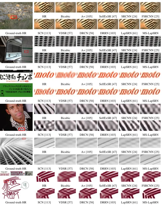
Table 3.6: Quantitative evaluation of state-of-the-art SR algorithms. We report the average PSNR/SSIM/IFC for 2×, 3×, and 4× SR. Red and blue
indicate the best and the second best performance, respectively. Both LapSRN [61] and the proposed MS-LapSRN do not use any 3× SR images for training. To generate the results of3×SR, we first perform
4×SR on input LR images and then downsample the output to the target resolution. . . 32 Table 3.7: Quantitative evaluation of state-of-the-art SR algorithms. We report
the average PSNR/SSIM/IFC for8×SR.Redandblueindicate the best and the second best performance, respectively. . . 33 Table 3.8: Quantitative comparisons between the generative network of the
LAPGAN [23] and our LapSRN.Our LapSRN achieves better recon-struction quality and faster processing speed than the LAPGAN. . . 39 Table 3.9: BT scores of SR algorithms in human subject study.Our MS-LapSRN
performs favorably against other compared methods. . . 43 Table 4.1: Quantitative evaluation on temporal warping error. The “Trained”
column indicates the applications used for training our model. Our method achieves a similarly reduced temporal warping error as Bon-neel et al. [11], which is significantly less than the original processed video (Vp). . . 62
Table 4.2: Quantitative evaluation on perceptual distance. Our method has lower perceptual distance than Bonneel et al. [11]. . . 63 Table 5.1: Ablation study. The baseline model is initialized from the pre-trained
SuperSloMo [54]. After training the model with the content loss LC,
perceptual loss LP, and the temporal loss LT, the image quality and
temporal stability are significantly improved. . . 81 Table 5.2: Human subject study. We conduct pairwise comparisons on 20 real
video. We show the percentage that users prefer our method against other approaches and the percentage of reasons when users select our method. . . 84
2012 B. S. in Electronics Engineering, National Taiwan Univer-sity, Taipei, Taiwan
2014 M. S. in Electronics Engineering, National Taiwan Univer-sity, Taipei, Taiwan
2019 Ph. D. in Electrical Engineering and Computer Science, Uni-versity of California, Merced
PUBLICATIONS
Wei-Sheng Lai, Deqing Sun, Jinwei Gu, Orazio Gallo, Ming-Hsuan Yang, and Jan Kautz,
Learning to Stitch Videos, in preparation for British Machine Vision Conference (BMVC),
2019.
Wenbo Bao, Wei-Sheng Lai, Chao Ma, Xiaoyun Zhang, Zhiyong Gao, and Ming-Hsuan Yang,Depth-Aware Video Frame Interpolation, IEEE Conference on Computer Vision and Pattern Recognition (CVPR), 2019.
Lerenhan Li, Jinshan Pan, Wei-Sheng Lai, Changxin Gao, Nong Sang, and Ming-Hsuan Yang, Blind Image Deblurring vis Deep Discriminative Priors, International Journal of Computer Vision (IJCV), 2019.
Wei-Sheng Lai, Jia-Bin Huang, Oliver Wang, Eli Shechtman, Ersin Yumer, and Ming-Hsuan Yang,Learning Blind Video Temporal Consistency, European Conference on Com-puter Vision (ECCV), 2018.
Xinyi Zhang, Hang Dong, Zhe Hu, Wei-Sheng Lai, Fei Wang, and Ming-Hsuan Yang,
Gated Fusion Network for Joint Image Deblurring and Super-Resolution, British Machine
Vision Conference (BMVC), 2018.
Wei-Sheng Lai, Jia-Bin Huang, Narendra Ahuja, and Ming-Hsuan Yang,Fast and Accurate
Image Super-Resolution with Deep Laplacian Pyramid Networks, IEEE Transactions on
Pattern Analysis and Machine Intelligence (TPAMI), 2018.
Ziyi Shen, Wei-Sheng Lai, Tingfa Xu, Jan Kautz, and Ming-Hsuan Yang,Deep Semantic
Face Deblurring, IEEE Conference on Computer Vision and Pattern Recognition (CVPR),
2018.
Lerenhan Li, Jinshan Pan, Wei-Sheng Lai, Changxin Gao, Nong Sang, and Ming-Hsuan Yang,Learning a Discriminative Prior for Blind Image Deblurring, IEEE Conference on Computer Vision and Pattern Recognition (CVPR), 2018.
Wei-Sheng Lai, Jia-Bin Huang, and Ming-Hsuan Yang,Semi-Supervised Learning for
Op-tical Flow with Generative Adversarial Networks, Neural Information Processing Systems
(NIPS), 2017.
Wei-Sheng Lai, Yujia Huang, Neel Joshi, Chris Buehler, Ming-Hsuan Yang and Sing Bing Kang, Semantic-driven Generation of Hyperlapse from 360-Degree Video, IEEE Transac-tions on Visualization and Computer Graphics (TVCG), 2017.
Wei-Sheng Lai, Jia-Bin Huang, Narendra Ahuja, and Ming-Hsuan Yang,Deep Laplacian
Pyramid Networks for Fast and Accurate Super-Resolution, IEEE Conference on Computer
Vision and Pattern Recognition (CVPR), 2017.
Jiawei Zhang, Jinshan Pan, Wei-Sheng Lai, Rynson Lau, Ming-Hsuan Yang, Learning
Fully Convolutional Networks for Iterative Non-blind Deconvolution, IEEE Conference
on Computer Vision and Pattern Recognition (CVPR), 2017.
Wei-Sheng Lai, Jia-Bin Huang, Zhe Hu, and Ming-Hsuan Yang,A Comparative Study for
Single-Image Blind Deblurring, IEEE Conference on Computer Vision and Pattern
Recog-nition (CVPR), 2016.
Learning Spatial and Temporal Visual Enhancement
by Wei-Sheng Lai
Doctor of Philosophy in Electrical Engineering and Computer Science University of California Merced, 2019
Professor Ming-Hsuan Yang, Chair
Visual enhancement is concerned with problems to improve the visual quality and view-ing experience for images and videos. Researchers have been actively workview-ing on this area due to its theoretical and practical interest. However, obtaining high visual quality often comes with a cost of computational efficiency. With the growth of mobile applications and cloud services, it is crucial to develop effective and efficient algorithms for generating visually attractive images and videos. In this thesis, we address the visual enhancement problems in three aspects, including the spatial, temporal, and the joint spatial-temporal domains. We propose efficient algorithms based on deep convolutional neural networks for solving various visual enhancement problems.
First, we address the problem ofspatialenhancement for single-image super-resolution. We propose a deep Laplacian Pyramid Network to reconstruct a high-resolution image from an input low-resolution input in a coarse-to-fine manner. Our model directly extracts fea-tures from input LR images and progressively reconstructs the sub-band residuals. We train the proposed model with a multi-scale training, deep supervision, and robust loss functions to achieve the state-of-the-art performance. Furthermore, we exploit the recursive learning technique to share parameters across and within pyramid levels to significantly reduce the model parameters. As most of the operations are performed on a low-resolution space, our model requires less memory and runs faster than state-of-the-art methods.
Second, we address thetemporalenhancement problem by learning the temporal con-sistency in videos. Given an input video and a per-frame processed video (processed by an existing image-based algorithm), we learn a recurrent network to reduce the temporal
flickering and generate a temporally consistent video. We train the proposed network by minimizing both short-term and long-term temporal losses as well as a perceptual loss to strike a balance between temporal coherence and perceptual similarity with the processed frames. At test time, our model does not require computing optical flow and thus runs at 400+ FPS on GPU for high-resolution videos. Our model is task independent, where a single model can handle multiple and unseen tasks, including but not limited to artistic style transfer, enhancement, colorization, image-to-image translation and intrinsic image decomposition.
Third, we address thespatial-temporalenhancement problem for video stitching. In-spired by the pushbroom cameras, we cast the stitching as a spatial interpolation problem. We propose a pushbroom stitching network to learn dense flow fields to smoothly align the input videos. The stitched videos can be generated from an efficient pushbroom in-terpolation layer. Our approach generates more temporally stable and visually pleasing results than existing video stitching approaches and commercial software. Furthermore, our algorithm has immediate applications in many areas such as virtual reality, immersive telepresence, autonomous driving, and video surveillance.
Introduction
1.1
Overview
With the growth of mobile cameras (e.g., smart phones, GoPro, and360◦ camera) and the wide spread of social media (e.g., Facebook, Instagram, and YouTube), millions of photos and videos are captured and uploaded to the Internet every day. However, many photos may suffer from artifacts (i.e., blurriness, noise, low spatial resolutions, or temporal flickering) or visual obstructions (i.e., limited field-of-view, reflection or occlusion). To address these issues, several problems have been studied in the field of computer vision, such as image super-resolution, motion deblurring, inpainting, video frame interpolation and video stitching and stabilization.
Conventional algorithms typically rely on a variety of priors or assumptions, e.g., total variation, sparse representation, self-similarity, brightness constancy and spatial smooth-ness, and develop complex optimization frameworks to solve the visual enhancement prob-lems. In recent years, data-driven approaches have been shown more effective to learn priors from a large image or video datasets. In particular, the deep convolutional neural networks (CNNs) have demonstrated great performance in many high-level as well as low-level vision problems due to its strong learning capacity. In this thesis, we propose efficient algorithms based on deep CNNs for solving visual enhancement problems in the following three aspects.
2
Spatial enhancement. Existing CNN-based single image super-resolution algorithms typically require a large number of network parameters and entail heavy computational loads for generating high-accuracy super-resolution results. Therefore, we propose a deep Laplacian Pyramid Network which performs fast and accurate single-image super-resolution.
Temporal enhancement. Applying image-based algorithms independently to each frame of a video often leads to temporally inconsistent results. On the other hand, task-specific video-based algorithms usually cannot be applied or generalized to different applications. Therefore, we propose a learning-based task-independent approach with a deep recurrent network for enforcing temporal consistency in a video.
Spatial-temporal enhancement. Despite the long history of image and video stitching research, existing academic and commercial solutions still produce strong artifacts due to the challenges of handling parallax. To address these issues, we propose a pushbroom stitching network by casting the stitching as a spatial interpolation problem.
1.2
Organization
In Chapter 2, we review and discuss the pros and cons of existing methods in the above three aspects.
In Chapter 3, we propose a deep Laplacian Pyramid Super-Resolution Network (Lap-SRN) that has both high reconstruction accuracy and fast execution speed to perform single-image super-resolution. Our model directly extracts features from the input LR single-images and progressively reconstructs the sub-band residuals of high-resolution images in a coarse-to-fine manner. Furthermore, we adopt a multi-scale deep supervision and a robust loss function to improve the reconstruction accuracy. As most of the operations are performed on a low-resolution space, our LapSRN requires less memory and runs faster than state-of-the-art methods. We further extend our LapSRN to incorporate recursive layers, local skip connections and multi-scale training to significantly improve the performance. By sharing parameters across and within pyramid levels, we reduce 73% of the network parameters while achieving better reconstruction accuracy. Extensive quantitative and qualitative eval-uations on benchmark datasets demonstrate that the proposed algorithm performs favorably
against the state-of-the-art methods in terms of speed and accuracy.
In Chapter 4, we propose a generic approach with a deep recurrent network to reduce the temporal flickering in a per-frame processed video. Our model takes as inputs the orig-inal and per-frame processed videos (processed by an existing image-based algorithm) and generate a temporally consistent video. We train the proposed network by minimizing both short-term and long-term temporal losses as well as a perceptual loss to strike a balance between temporal coherence and perceptual similarity with the processed frames. At test time, our model does not require computing optical flow and thus runs at 400+ FPS on GPU for high-resolution videos. The proposed method is agnostic to specific image processing algorithms applied to the original video. Therefore, a single model can handle multiple and unseen tasks, including but not limited to artistic style transfer, enhancement, colorization, image-to-image translation and intrinsic image decomposition.
In Chapter 5, we propose a video stitching algorithm that is temporally stable and toler-ant to strong parallax. Our key insight is that stitching can be cast as a problem of learning a smooth spatial interpolation between the input videos, inspired by the pushbroom cameras. We introduce a fast pushbroom interpolation layer and propose a novel pushbroom stitching network, which learns a dense flow field to smoothly align the input videos. Our approach generates more visually pleasing results than existing approaches and has immediate appli-cations in many areas such as virtual reality, immersive telepresence, autonomous driving, and video surveillance.
In Chapter 6, we conclude the contributions in this thesis and discuss several future re-search directions, including the practical applications of low-level vision, semi-supervised learning and domain adaptation, and learning-based computational photography.
Chapter 2
Literature Review
In this chapter, we review the literature related to the research work presented in the following chapters.
2.1
Single Image Super-Resolution
Single-image super-resolution has been extensively studied in the literature [120]. Here we focus our discussion on recent example-based and CNN-based approaches.
2.1.1
SR Using Internal Databases
Several methods [31, 119, 35] exploit the self-similarity property in natural images and construct LR-HR patch pairs based on the scale-space pyramid of the LR input im-age. While internal databases contain more relevant training patches than external image datasets, the number of LR-HR patch pairs may not be sufficient to cover large textural ap-pearance variations in an image. Singh et al. [100] decompose patches into directional fre-quency sub-bands and determine better matches in each sub-band pyramid independently. Huang et al. [47] extend the patch search space to accommodate the affine and perspective deformation. The SR methods based on internal databases are typically slow due to the heavy computational cost of patch searches in the scale-space pyramid. Such drawbacks make these approaches less feasible for applications that require computational efficiency.
2.1.2
SR Using External Databases
Numerous SR methods learn the LR-HR mapping with image pairs collected from ex-ternal databases using supervised learning algorithms, such as nearest neighbor [32], man-ifold embedding [8, 18], kernel ridge regression [59], and sparse representation [122, 123, 128]. Instead of directly modeling the complex patch space over the entire database, recent methods partition the image set by K-means [121], sparse dictionary [106, 105] or random forest [95], and learn locally linear regressors for each cluster. While these approaches are effective and efficient, the extracted features and mapping functions are hand-designed, which may not be optimal for generating high-quality SR images.
2.1.3
CNN-based SR
CNN-based SR methods have demonstrated state-of-the-art results by jointly optimiz-ing the feature extraction, non-linear mappoptimiz-ing, and image reconstruction stages in an end-to-end manner. The VDSR network [57] shows significant improvement over the SRCNN method [24] by increasing the network depth from 3 to 20 convolutional layers. To fa-cilitate training a deeper model with a fast convergence speed, the VDSR method adopts the global residual learning paradigm to predict the differences between the ground truth HR image and the bicubic upsampled LR image instead of the actual pixel values. Wang et al. [113] combine the domain knowledge of sparse coding with a deep CNN and train a cascade network (SCN) to upsample images progressively. In [58], Kim et al. propose a network with multiple recursive layers (DRCN) with up to 16 recursions. The DRRN approach [103] further trains a 52-layer network by extending the local residual learning approach of the ResNet [41] with deep recursion. We note that the above methods use bicu-bic interpolation to pre-upsample input LR imagesbefore feeding into the deep networks, which increases the computational cost and requires a large amount of memory.
To achieve real-time speed, the ESPCN method [98] extracts feature maps in the LR space and replaces the bicubic upsampling operation with an efficient sub-pixel convolution (i.e., pixel shuffling). The FSRCNN method [25] adopts a similar idea and uses a hourglass-shaped CNN with transposed convolutional layers for upsampling. As a trade-off of speed, both ESPCN [98] and FSRCNN [25] have limited network capacities for learning complex mappings. Furthermore, these methods upsample images or features in one upsampling
6
stepand use only one supervisory signal from the target upsampling scale. Such a design often causes difficulties in training models for large upsampling scales (e.g.,4×or8×). In contrast, our model progressively upsamples input images onmultiplepyramid levels and usemultiplelosses to guide the prediction of sub-band residuals at each level, which leads to accurate reconstruction, particularly for large upsampling scales.
All the above CNN-based SR methods optimize networks with the L2 loss function,
which often leads to over-smooth results that do not correlate well with human perception. We demonstrate that the proposed deep network with the robust Charbonnier loss func-tion better handles outliers and improves the SR performance over the L2 loss function.
Most recently, Lim et al. [75] propose a multi-scale deep SR model (MDSR) by extend-ing ESPCN [98] with three branches for scale-specific upsamplextend-ing but sharextend-ing most of the parameters across different scales. The MDSR method is trained on a high-resolution DIV2K [104] dataset (800 training images of 2k resolution), and achieves the state-of-the-art performance. Table 2.1 shows the main components of the existing CNN-based SR methods. The proposed LapSRN and MS-LapSRN are listed on the last two rows.
2.1.4
Laplacian Pyramid
The Laplacian pyramid has been widely used in several vision tasks, including image blending [15], texture synthesis [43], edge-aware filtering [84] and semantic segmenta-tion [34]. Denton et al. [23] propose a generative adversarial network based on a Laplacian pyramid framework (LAPGAN) to generate realistic images, which is the most related to our work. However, the proposed LapSRN differs from LAPGAN in two aspects.
First, the objectives of the two models are different. The LAPGAN is a generative model which is designed to synthesize diverse natural images from random noise and sam-ple inputs. On the contrary, the proposed LapSRN is a super-resolution model that predicts a particular HR image based on the given LR image and upsampling scale factor. The LAP-GAN uses a cross-entropy loss function to encourage the output images to respect the data distribution of the training datasets. In contrast, we use the Charbonnier penalty function to penalize the deviation of the SR prediction from the ground truth HR images.
Second, the differences in architecture designsresult in disparate inference speed and network capacities. The LAPGAN upsamples input images before applying convolution
Table 2.1: Feature-by-feature comparisons of CNN-based SR algorithms. Methods with direct reconstruction performs one-step upsampling from the LR to HR space, while progressive reconstruction predicts HR images in multiple upsampling steps. Depth repre-sents the number of convolutional and transposed convolutional layers in the longest path from input to output for4×SR. Global residual learning (GRL) indicates that the network learns the difference between the ground truth HR image and the upsampled (i.e., using bicubic interpolation or learned filters) LR images. Local residual learning (LRL) stands for the local skip connections between intermediate convolutional layers.
Method Input Depth Filters Parameters GRL LRL Multi-scale Loss function training SRCNN [24] LR + bicubic 3 64 57k L2 FSRCNN [25] LR 8 56 12k L2 ESPCN [98] LR 3 64 20k L2 SCN [113] LR + bicubic 10 128 42k L2 VDSR [57] LR + bicubic 20 64 665k X X L2 DRCN [58] LR + bicubic 20 256 1775k X L2 DRRN [103] LR + bicubic 52 128 297k X X X L2 MDSR [75] LR 162 64 8000k X X Charbonnier
LapSRN (ours) LR 24 64 812k X Charbonnier
8
at each level, while our LapSRN extracts features directly from the LR space and upscales images at the end of each level. Our network design effectively alleviates the computational cost and increases the size of receptive fields. In addition, the convolutional layers at each level in our LapSRN areconnectedthrough multi-channel transposed convolutional layers. The residual images at a higher level are therefore predicted by a deeper network with shared feature representations at lower levels. The shared features at lower levels increase the non-linearity at finer convolutional layers to learn complex mappings.
2.1.5
Adversarial Training
The Generative Adversarial Networks (GANs) [36] have been applied to several im-age reconstruction and synthesis problems, including imim-age inpainting [86], face comple-tion [74], and face super-resolucomple-tion [126]. Ledig et al. [66] adopt the GAN framework for learning natural image super-resolution. The ResNet [41] architecture is used as the generative network and train the network using the combination of the L2 loss,
percep-tual loss [56], and adversarial loss. The SR results may have lower PSNR but are visually plausible. Note that our LapSRN can be easily extended to incorporate adversarial training.
2.2
Video Temporal Consistency
We address the temporal consistency problem on a wide range of applications, includ-ing automatic white balancinclud-ing [44], harmonization [9], dehazinclud-ing [39], image enhance-ment [33], style transfer [48, 56, 72], colorization [50, 130], image-to-image translation [52, 132], and intrinsic image decomposition [7]. In the following, we discuss task-specific and task-independent approaches that enforce temporal consistency on videos.
2.2.1
Task-Specific Approaches
A common solution to embed the temporal consistency constraint is to use optical flow to propagate information between frames, e.g., colorization [71] and intrinsic decompo-sition [125]. However, estimating optical flow is computationally expensive and thus is impractical to apply on high-resolution and long sequences. Temporal filtering is an effi-cient approach to extend image-based algorithms to videos, e.g., tone-mapping [5], color
Table 2.2: Comparison of blind temporal consistency methods. Both the methods of Bonneel et al. [11] and Yao et al. [124] require dense correspondences from optical flow or PatchMatch [6], while the proposed method does not explicitly rely on these correspon-dences at test time. The algorithm of Yao et al. [124] involves a key-frame selection from the entire video and thus cannot generate output in an online manner.
Bonneel et al. [11] Yao et al. [124] Ours Content constraint gradient local affine perceptual loss
Short-term temporal constraint X - X
Long-term temporal constraint - X X
Require dense correspondences at test time X X
-Online processing X - X
transfer [10], and visual saliency [65] to generate temporally consistent results. Neverthe-less, these approaches assume a specific filter formulation and cannot be generalized to other applications.
Recently, several approaches have been proposed to improve the temporal stability of CNN-based image style transfer. Huang et al. [45] and Gupta et al. [37] train feed-forward networks by jointly minimizing content, style and temporal warping losses. These methods, however, are limited to the specific styles used during training. Chen et al. [19] learn flow and mask networks to adaptively blend the intermediate features of the pre-trained style network. While the architecture design is independent of the style network, it requires the access to intermediate features and cannot be applied to non-differentiable tasks. In contrast, the proposed model is entirely blind to specific algorithms applied to the input frames and thus is applicable to optimization-based techniques, CNN-based algorithms, and combinations of Photoshop filters.
2.2.2
Task-Independent Approaches
Several methods have been proposed to improve temporal consistency for multiple tasks. Lang et al. [65] approximate global optimization of a class of energy formulation (e.g., colorization, optical flow estimation) via temporal edge-aware filtering. In [26], Dong et al. propose a segmentation-based algorithm and assume that the image transformation
10
is spatially and temporally consistent. More general approaches assume gradient similar-ity [11] or local affine transformation [124] between the input and the processed frames. These methods, however, cannot handle more complicated tasks (e.g., artistic style trans-fer). In contrast, we use the VGG perceptual loss [56] to impose high-level perceptual similarity between the output and processed frames. We list the feature-by-feature compar-isons between Bonneel et al. [11], Yao et al. [124] and the proposed method in Table 2.2.
2.3
Video Stitching
We first review the most relevant work on image and video stitching and then discuss the conventional pushbroom camera, which inspires the proposed algorithm.
2.3.1
Image Stitching
Existing image stitching methods often build on the conventional pipeline of Brown and Lowe et al. [13], which first estimates a 2D transformation (e.g., homography) for align-ment and then stitches images using the seam-cutting [28] or multi-band blending [16]. However, ghosting artifacts and mis-alignment still exist, especially when input images have large parallax. To account for parallax, several methods adopt spatially varying local warping based on the affine [78] or projective [127] transformations. Zhang et al. [129] integrate the content-preserving warping and seam-cutting algorithms to handle parallax while avoiding local distortions. More recent methods combine the homography and simi-larity transforms [17, 76] to reduce the projective distortion (i.e., stretched shapes) or adopt a global similarity prior [22] to preserve the global shape of the whole stitched images.
While the above techniques are effective at creating a panorama from still images, ap-plying these algorithms to stitch a video frame-by-frame results in a significant amount of temporal instability. In contrast, the proposed algorithm stitches each frame individually but is able to generate spatio-temporally coherent stitched videos due to the design of the pushbroom interpolation layer.
2.3.2
Video Stitching
Due to computational efficiency, it is not straightforward to enforce spatio-temporal consistency in existing image stitching algorithms. Commercial software, e.g., VideoS-titch Studio [110] or AutoPano Video [4], often finds a fixed transformation (with camera calibration) to align all the frames, but cannot align local content well. Recent methods integrate local warping and optical flow [89] or find a spatio-temporal content-preserving warping [55] to stitch videos, which are computationally expensive. Lin et al. [77] stitch videos captured from hand-held cameras based on 3D scene reconstruction, which is also time-consuming. On the other hand, several approaches, e.g., Rich360 [69] and Google Jump [2], create360◦ videos from multiple videos captured on a structured rig. Recently, NVIDIA provides a toolkit, VRWorks [83], to efficiently stitch videos based on depth and motion estimation. Still several artifacts, e.g., broken objects and ghosting, are visible on the stitched video.
Different from existing methods, the proposed algorithm learns locally adaptive warp-ing based on a deep CNN to effectively and efficiently align the input views. The warpwarp-ing is learned to optimize the quality of the stitched video in an end-to-end fashion.
2.3.3
Pushbroom Panorama
The linear pushbroom camera [38] is mounted on a moving platform, e.g., satellite, and moves along a straight line. At each time stamp, the sensor captures 1D images of the viewing plane, e.g., surface of the earth. The stack of these 1D images constitutes the 2D panoramic image. The pushbroom camera has been widely used to create satellite images or panorama for street scenes [96]. It works well when the scene is far from the sensor or has nearly uniform depth. However, distortions (e.g., stretched or squashed objects) appear when the captured scene has large depth variations or dynamic objects. Several methods handle this issue by estimating scene depth [92], finding a cutting-seam on the space-time volume [114], or optimizing the viewpoint for each pixel [1].
The proposed method is a software simulation of the pushbroom camera to create panoramas and synthesizes the scan of a scene through spatial interpolation. We further use a refinement network to reduce artifacts created by the interpolation process and learn the entire model end-to-end to optimize the stitched view from a realistic synthetic dataset.
Chapter 3
Fast and Accurate Image
Super-Resolution with Deep Laplacian
Pyramid Networks
3.1
Introduction
Single image super-resolution (SR) aims to reconstruct a high-resolution (HR) im-age from one single low-resolution (LR) input imim-age. Example-based SR methods have demonstrated the state-of-the-art performance by learning a mapping from LR to HR im-age patches using large imim-age datasets. Numerous learning algorithms have been applied to learn such a mapping function, including dictionary learning [122, 123], local linear regression [105, 121], and random forest [95], to name a few.
Convolutional Neural Networks (CNNs) have been widely used in vision tasks rang-ing from object recognition [41], segmentation [79], optical flow [30], to super-resolution. In [24], Dong et al. propose a Super-Resolution Convolutional Neural Network (SRCNN) to learn a nonlinear LR-to-HR mapping function. This network architecture has been ex-tended to embed a sparse coding model [113], increase network depth [57], or apply re-cursive layers [58, 103]. While these models are able to generate high-quality SR images, there remain three issues to be addressed. First, these methods use a pre-defined upsam-pling operator, e.g.bicubic interpolation, to upscale an input LR image to the desired spatial resolution beforeapplying a network for predicting the details (Figure 3.1(a)). This
upsampling step increases unnecessary computational cost and does not provide additional high-frequency information for reconstructing HR images. Several algorithms accelerate the SRCNN by extracting features directly from the input LR images (Figure 3.1(b)) and re-placing the pre-defined upsampling operator with sub-pixel convolution [98] or transposed convolution [25] (also named as deconvolution in some literature). These methods, how-ever, use relatively small networks and cannot learn complicated mappings well due to the limited model capacity. Second, existing methods optimize the networks with anL2 loss
(i.e., mean squared error loss). Since the same LR patch may have multiple corresponding HR patches and theL2loss fails to capture the underlying multi-modal distributions of HR
patches, the reconstructed HR images are often over-smoothed and inconsistent to human visual perception on natural images. Third, existing methods mainly reconstruct HR im-ages in one upsampling step, which makes learning mapping functions for large scaling factors (e.g.,8×) more difficult.
To address these issues, we propose the deep Laplacian Pyramid Super-Resolution Net-work (LapSRN) to progressively reconstruct HR images in a coarse-to-fine fashion. As shown in Figure 3.1(c), our model consists of a feature extraction branch and an image reconstruction branch. The feature extraction branch uses a cascade of convolutional lay-ers to extract non-linear feature maps from LR input images. We then apply a transposed convolutional layer for upsampling the feature maps to a finer level and use a convolutional layer to predict the sub-band residuals (i.e., the differences between the upsampled image and the ground truth HR image at the respective pyramid level). The image reconstruc-tion branch upsamples the LR images and takes the sub-band residuals from the feature extraction branch to efficiently reconstruct HR images through element-wise addition. Our network architecture naturally accommodates deep supervision (i.e., supervisory signals can be applied simultaneously at each level of the pyramid) to guide the reconstruction of HR images. Instead of using theL2loss function, we propose to train the network with the
robust Charbonnier loss functions to better handle outliers and improve the performance. While both feature extraction and image reconstruction branches have multiple levels, we train the network in an end-to-end fashion without stage-wise optimization.
Our algorithm differs from existing CNN-based methods in the following three aspects: 1. Accuracy. Instead of using a pre-defined upsampling operation, our network jointly optimizes the deep convolutional layers and upsampling filters for both images and
14
bicubic interpolation
...
...
(a) Pre-upsampling (b) Post-upsampling
+
+ +
...
...
...
Feature Extraction Branch
Image Reconstruction Branch
(c) Progressive upsampling (ours)
Figure 3.1: Comparisons of upsampling strategies in CNN-based SR algorithms. Red arrows indicate convolutional layers. Blue arrows indicate transposed convolutions (up-sampling), and green arrows denote element-wise addition operators. (a) Pre-upsampling based approaches (e.g., SRCNN [24], VDSR [57], DRCN [58], DRRN [103]) typically use the bicubic interpolation to upscale LR input images to the target spatial resolution be-fore applying deep networks for prediction and reconstruction. (b) Post-upsampling based methods directly extract features from LR input images and use sub-pixel convolution [98] or transposed convolution [25] for upsampling. (c) Progressive upsampling approach us-ing the proposed Laplacian pyramid network reconstructs HR images in a coarse-to-fine manner.
feature maps by minimizing the Charbonnier loss function. As a result, our model has a large capacity to learn complicated mappings and effectively reduces the undesired artifacts caused by spatial aliasing.
2. Speed. Our LapSRN accommodates both fast processing speed and high capac-ity of deep networks. Experimental results demonstrate that our method is faster than several CNN-based super-resolution models, e.g., VDSR [57], DRCN [58], and DRRN [103]. The proposed model achieves real-time performance as FSRCNN [25] while generating significantly better reconstruction accuracy.
3. Progressive reconstruction. Our model generates multiple intermediate SR predic-tions inonefeed-forward pass through progressive reconstruction. This characteristic renders our method applicable to a wide range of tasks that require resource-aware adaptability. For example, the same network can be used to enhance the spatial res-olution of videos depending on the available computational resources. For scenarios with limited computing resources, our8×model can still perform 2×or4×SR by simply bypassing the computation of residuals at finer levels. Existing CNN-based methods, however, do not offer such flexibility.
In addition, we exploit the following techniques to substantially improve our LapSRN: 1. Parameter sharing. We re-design our network architecture to share parameters
across pyramid levels and within the feature extraction sub-network via recursion.
Through parameter sharing, we reduce73%of the network parameters while achiev-ing better reconstruction accuracy on benchmark datasets.
2. Local skip connections. We systematically analyze three different approaches for applying local skip connections in the proposed model. By leveraging proper skip connections to alleviate the gradient vanishing and explosion problems, we are able to train an 84-layer network to achieve the state-of-the-art performance.
3. Multi-scale training. Unlike in the preliminary work where we train three different models for handling 2×, 4× and 8× SR, respectively, we train one single model to handlemultiple upsampling scales. The multi-scale model learns the inter-scale correlation and improves the reconstruction accuracy against single-scale models. We refer to our multi-scale model as MS-LapSRN.
16 + + LR input 4 ×SR output 2 ×SR output Conv୧୬ Image Upsampling Image Upsampling Feature Embedding Feature Upsampling Conv୰ୣୱ Feature Embedding Feature Upsampling Conv୰ୣୱ share parameters
Figure 3.2: Detailed network architecture of the proposed LapSRN. At each pyramid level, our model consists of a feature embedding sub-network for extracting non-linear features, transposed convolutional layers for upsampling feature maps and images, and a convolutional layer for predicting the sub-band residuals. As the network structure at each level is highly similar, we share the weights of those components across pyramid levels to reduce the number of network parameters.
3.2
Deep Laplacian Pyramid Network for SR
In this section, we describe the design methodology of the proposed LapSRN, including the network architecture, parameter sharing, loss functions, multi-scale training strategy, and details of implementation as well as network training.
3.2.1
Network Architecture
We construct our network based on the Laplacian pyramid framework. Our model takes an LR image as input (rather than an upscaled version of the LR image) and progressively predicts residual images on the log2S pyramid levels, where S is the upsampling scale factor. For example, our network consists of3 pyramid levels for super-resolving an LR image at a scale factor of8. Our model consists of two branches: (1) feature extraction and (2) image reconstruction.
Feature extraction branch. As illustrated in Figure 3.1(c) and Figure 3.2, the feature extraction branch consists of (1) a feature embedding sub-network for transforming high-dimensional non-linear feature maps, (2) a transposed convolutional layer for upsampling
the extracted features by a scale of 2, and (3) a convolutional layer (Convres) for predicting
the sub-band residual image. The first pyramid level has an additional convolutional layer (Convin) to extract high-dimensional feature maps from the input LR image. At other
levels, the feature embedding sub-network directly transforms features from the upscaled feature maps at the previous pyramid level. Unlike the design of the LAPGAN, we do not
collapsethe feature maps into an image before feeding into the next level. Therefore, the
feature representations at lower levels are connected to higher levels and thus can increase the non-linearity of the network to learn complex mappings at the finer levels. Note that we perform the feature extraction at the coarse resolution and generate feature maps at
the finer resolution with only one transposed convolutional layer. In contrast to existing
networks (e.g., [57, 103]) that perform all feature extraction and reconstruction at the finest resolution, our network design significantly reduces the computational complexity.
Image reconstruction branch. At level s, the input image is upsampled by a scale of 2 with a transposed convolutional layer, which is initialized with a 4×4 bilinear kernel. We then combine the upsampled image (using element-wise summation) with the predicted residual image to generate a high-resolution output image. The reconstructed HR image at levelsis then used as an input for the image reconstruction branch at levels+ 1. The entire network is a cascade of CNNs with the same structure at each level. We jointly optimize the upsampling layer with all other layers to learn better a upsampling function.
3.2.2
Feature Embedding Sub-network
In our preliminary work [61], we use a stack of multiple convolutional layers as our fea-ture embedding sub-network. In addition, we learn distinct sets of convolutional filters for feature transforming and upsampling at different pyramid levels. Consequently, the num-ber of network parameters increases with the depth of the feature embedding sub-network and the upsampling scales, e.g., the4×SR model has about twice number of parameters than the 2× SR model. We explore two directions to reduce the network parameters of LapSRN.
Parameter sharing across pyramid levels. Our first strategy is to share the network parameters across pyramid levels as the network at each level shares the same structure
18
and the task (i.e., predicting the residual images at2×resolution). As shown in Figure 3.2, we share the parameters of the feature embedding sub-network, upsampling layers, and the residual prediction layers across all the pyramid levels. As a result, the number of network parameters is independent of the upsampling scales. We can use a single set of parameters to construct multi-level LapSRN models to handle different upsampling scales.
Parameter sharing within pyramid level. Our second strategy is to share the network parameterswithineach pyramid level. Specifically, we extend the feature embedding sub-network using deeply recursive layers to effectively increase the sub-network depth without increasing the number of parameters. The design of recursive layers has been adopted by several recent CNN-based SR approaches. The DRCN method [58] applies a single
convolutional layer repeatedly up to 16 times. However, with a large number of filters (i.e., 256 filters), the DRCN is memory-demanding and slow at runtime. Instead of reusing the weights of a single convolutional layer, the DRRN [103] method shares the weights
of a block (2 convolutional layers with 128 filters). In addition, the DRRN introduces a
variant of local residual learning from the ResNet [41]. Specifically, the identity branch of the ResNet comes from the output of the previous block, while the identity branch of the DRRN comes from the input of the first block. Such a local skip connection in the DRRN creates multiple short paths from input to output and thereby effectively alleviates the gradient vanishing and exploding problems. Therefore, DRRN has 52 convolutional layers with only 297k parameters.
In the proposed LapSRN, the feature embedding sub-network has Rrecursive blocks. Each recursive block has D distinct convolutional layers, which controls the number of parameters in the entire model. The weights of the D convolutional layers are shared among the recursive blocks. Given an upsampling scale factorS, the depth of the LapSRN can be computed by:
depth= (D×R+ 1)×L+ 2, (3.1) whereL = log2S. The 1within the parentheses represents the transposed convolutional layers, and the2at the end of (3.1) represents the first convolutional layer applied on input images and the last convolutional layer for predicting residuals. Here we define the depth of a network as the longest path from input to output.
+ + + ڭ Input Recursive Block Recursive Block Recursive Block + + + ڭ Input Recursive Block Recursive Block Recursive Block + + + ڭ Input Recursive Block Recursive Block Recursive Block
(a) No skip connection (b) Distinct-source skip connection (c) Shared-source skip connection
Figure 3.3: Local residual learning. We explore three different ways of local skip con-nection in the feature embedding sub-network for training deeper models.
Local residual learning. As the gradient vanishing and exploding problem are common issues when training deep models, we explore three different methods of local residual learning in our feature embedding sub-network to stabilize our training process:
1. No skip connection: A plain network without any local skip connection. We denote our LapSRN without skip connections as LapSRNNS.
2. Distinct-source skip connection: The ResNet-style local skip connection. We de-note our LapSRN with such skip connections as LapSRNDS.
3. Shared-source skip connection: The local skip connection introduced by DRRN [103]. We denote our LapSRN with such skip connections as LapSRNSS.
We illustrate the three local residual learning methods in Figure 3.3 and the detailed struc-ture of our recursive block in Figure 3.4. We use the pre-activation strucstruc-ture [42] without the batch normalization layer in our recursive block.
3.2.3
Loss Function
Let xbe the input LR image andθ be the set of network parameters to be optimized. Our goal is to learn a mapping functionf for generating an HR imageyˆ=f(x;θ)that is as
20 ڭ Recursive Block (ܦconvolutions) + Block input Skip connection ReLU Conv ReLU Conv Block output
Figure 3.4: Structure of our recursive block. There are D convolutional layers in a recursive block. The weights of convolutional layers are distinct within the block but shared among all recursive blocks.
similar to the ground truth HR imageyas possible. We denote the residual image at level
lbyrˆl, the upscaled LR image byxland the corresponding HR images byyˆl. The desired
output HR images at levellis modeled byyˆl =xl+ ˆrl. We use the bicubic downsampling
to resize the ground truth HR imageytoyl at each level. Instead of minimizing the mean square errors betweenyˆlandyl, we use a robust loss function to handle outliers. The overall
loss function is defined as:
LS(y,yˆ;θ) = 1 N N X i=1 L X l=1 ρyl(i)−yˆl(i) = 1 N N X i=1 L X l=1 ρ(yl(i)−xl(i))−rˆl(i), (3.2) whereρ(x) =√x2+2is the Charbonnier penalty function (a differentiable variant ofL
1
norm) [14],N is the number of training samples in each batch,S is the target upsampling scale factor, andL= log2Sis the number of pyramid levels in our model. We empirically setto1e−3.
ground truth HR imageys. This multi-loss structure resembles the deeply-supervised
net-works for classification [67] and edge detection [115]. The deep multi-scale supervision guides the network to reconstruct HR images in a coarse-to-fine fashion and reduce spatial aliasing artifacts.
3.2.4
Multi-Scale Training
The multi-scales SR models (i.e., trained with samples from multiple upsampling scales simultaneously) have been shown more effective than single-scale models as SR tasks have inter-scale correlations. For pre-upsampling based SR methods (e.g., VDSR [57] and DRRN [103]), the input and output of the network have the same spatial resolution, and the outputs of different upsampling scales are generated from the same layer of the network. In the proposed LapSRN, samples of different upsampling scales are generated from different layers and have different spatial resolutions. We use 2×, 4×, and8× SR samples to train a multi-scale LapSRN model. We construct a 3-level LapSRN model and minimize the combination of loss functions from three different scales:
L(y,yˆ;θ) = X
S∈{2,4,8}
LS(y,yˆ;θ). (3.3)
We note that the pre-upsampling based SR methods could apply scale augmentation for arbitrary upsampling scales, while in our LapSRN, the upsampling scales for training are limited to2n×SR wherenis an integer.
3.2.5
Implementation and Training Details
In the proposed LapSRN, we use 64 filters in all convolutional layers except the first layer applied on the input LR image, the layers for predicting residuals, and the image upsampling layer. The filter size of the convolutional and transposed convolutional layers are 3×3 and 4×4, respectively. We pad zeros around the boundaries before applying convolution to keep the size of all feature maps the same as the input of each level. We initialize the convolutional filters using the method of He et al. [40] and use the leaky rectified linear units (LReLUs) [80] with a negative slope of 0.2 as the non-linear activation function.
22
We use 91 images from Yang et al. [123] and 200 images from the training set of the Berkeley Segmentation Dataset [3] as our training data. The training dataset of 291 images is commonly used in the state-of-the-art SR methods [57, 95, 61, 103]. We use a batch size of 64 and crop the size of HR patches to 128×128. An epoch has 1,000 iterations of back-propagation. We augment the training data in three ways: (1)Scaling: randomly downscale images between[0.5,1.0]; (2)Rotation: randomly rotate image by90◦,180◦, or
270◦; (3)Flipping: flip images horizontally with a probability of0.5. Following the training protocol of existing methods [24, 57, 103], we generate the LR training patches using the bicubic downsampling. We use the MatConvNet toolbox [109] and train our model using the Stochastic Gradient Descent (SGD) solver. In addition, we set the momentum to 0.9
and the weight decay to1e−4. The learning rate is initialized to1e−5for all layers and decreased by a factor of 2 for every 100 epochs.
3.3
Discussions and Analysis
In this section, we first validate the contributions of different components in the pro-posed network. We then discuss the effect of local residual learning and parameter sharing in our feature embedding sub-network. Finally, we analyze the performance of multi-scale training strategy.
3.3.1
Model Design
We train a LapSRN model with 5 convolutional layers (without parameters sharing and the recursive layers) at each pyramid level to analyze the performance of pyramid network structure, global residual learning, robust loss functions, and multi-scale supervision.
Pyramid structure. By removing the pyramid structure, our model falls back to a net-work similar to the FSRCNN but with the global residual learning. We train this netnet-work using 10 convolutional layers in order to have the same depth as our LapSRN. Figure 3.5 shows the convergence curves in terms of PSNR on the SET14 for4×SR. The quantitative
results in Table 3.1 and Figure 3.6 show that the pyramid structure leads to considerable performance improvement (e.g., 0.7 dB on SET5 and 0.4 dB on SET14), which validates
Epoch
0
50
100
150
PSNR (dB)
26.6
27
27.4
27.8
28.2
SRCNN FSRCNNw/o pyramid structure w/o residual learning w/o robust loss LapSRN (full model)
Figure 3.5:Convergence analysis. We analyze the contributions of the pyramid structures, loss functions, and global residual learning by replacing each component with the one used in existing methods. Our full model converges faster and achieves better performance. Table 3.1: Ablation study of LapSRN.Our full model performs favorably against several variants of the LapSRN on both SET5 and SET14 for4×SR.
GRL Pyramid Loss SET5 SET14
X Charbonnier 30.58 27.61
X Charbonnier 31.10 27.94
X X L2 30.93 27.86
X X Charbonnier 31.28 28.04
the effectiveness of our Laplacian pyramid network design.
Global residual learning. To demonstrate the effectiveness of global residual learning, we remove the image reconstruction branch and directly predict the HR images at each level. In Figure 3.5, the performance of the non-residual network (blue curve) converges slowly and fluctuates significantly during training. Our full LapSRN model (red curve), on the other hand, outperforms SRCNN within 10 epochs.
Loss function. To validate the effectiveness of the Charbonnier loss function, we train the proposed network with conventional L2 loss function. We use a larger learning rate
24
(a) (b) (c) (d) (e) (f)
Figure 3.6: Contribution of different components in LapSRN. (a) Ground truth HR image (b) without pyramid structure (c) without global residual learning (d) without robust loss (e) full model (f) HR patch.
Ground-truth HR
LR 2×SR w/o M.S. 4×SR w/o M.S.
HR 2×SR w/ M.S. 4×SR w/ M.S.
Figure 3.7: Contribution of multi-scale supervision (M.S.). The multi-scale supervision guides the network training to progressively reconstruct the HR images and help reduce the spatial aliasing artifacts.