Dottorato di Ricerca in Statistica Metodologica
Tesi di Dottorato - XXIX Ciclo - anno 2017
Dipartimento di Scienze Statistiche
Spatial analysis of photoreceptor mosaic
from Adaptive Optics images of the
human retina
Thesis Supervisor:
Dottoranda:
Chiar.mo Prof.
Ing. Daniela Giannini
L’occhio, che si dice finestra dell’anima, è la principale via donde il comune senso
può più copiosamente e magnificamente considerare le infinite opere di natura.
Trattato della pittura, Leonardo Da Vinci
A tutte le persone che lasciano il cammino della vita
1
Index
Chapter 1
The eye and the adaptive optics retinal imaging
1.1The eye: how we see ... 5
1.2 The retina ... 6
1.3 Phototransduction ... 9
1.4 The Optical System of the Human Eye ... 14
1.5 Adaptive Optics Technology for Retinal Imaging ... 15
1.6 rtx1; Adaptive Optics Retinal Camera ... 17
1.7 The Photoreceptor Mosaic and degenerative diseases of the human retina ... 19
1.8 Summary of dissertation aim ... 22
Chapter 2 Reliability and agreement between metrics of cone spacing in adaptive optics images of the human retinal photoreceptor mosaic 2.1 Introduction ... 24
2.2 Methods ... 25
2.2.1 Human subjects ... 26
2.2.2 Image acquisition and processing... 27
2.2.3 Density and packing arrangement metrics of the cone mosaic ... 28
2.2.4 Spacing metrics of the cone mosaic ... 28
2.2.5 Statistics ... 31
2.3 Results ... 31
2.3.1 Cone density and packing arrangement ... 31
2.3.2 Cone spacing metrics ... 33
2.3.2.1 Agreement and correlation between spacing metrics ... 33
2.3.2.2 Influence of the sampling area on Scc... 36
2.3.2.3 Influence of the sampling area on LCS ... 37
2.3.2.4 Influence of the sampling area on DRPD ... 37
2.4 Discussion ... 38
Chapter 3 Statistical analysis of second-order properties of cone mosaic 3.1 Introduction ... 42
3.2 Methods ... 44
2
3.2.2 Image acquisition and processing: Real data ... 44
3.2.3 Generation of Simulated data ... 46
3.2.4 Spatial statistics ... 46
3.2.4.1 Intensity estimation ... 48
3.2.4.2 Nearest Neighbour Distance Function G... 49
3.2.4.3 K and L Functions ... 49
3.2.4.4 Pair correlation function g2(r) and Structure factor: s(k) ... 50
3.2.5 Statistical methodology ... 52
3.2.6 Summary characteristics ... 52
3.3 Results ... 53
3.4 Discussion ... 57
Chapter 4 Clustering of spatial functions profiles extracted from normal and diseased AO cone mosaics 4.1 Introduction ... 66
4.2 Methods ... 66
4.2.1 Trend ... 66
4.2.2 Velocity and acceleration ... 67
4.2.3 Dissimilarity matrix... 68 4.2.4 Dataset ... 70 4.3 Results ... 70 4.4 Discussion ... 73 Conclusion ... 75 Bibliography ... 76
3
LIST OF ABBREVIATIONS
RGC - retina ganglion cells RNFL - retinal nerve fibre layer ONH - optic nerve head
ONL - outer nuclear layer INL - inner nuclear layer GCL - ganglion cell layer OPL - outer plexiform layer IPL - inner plexiform layer OS - outer segment
IS - inner segment
ATP - adenosine triphosphate
cGMP - cyclic guanosine monophosphate LOA - low-order aberrations
HOA - high-order aberrations WA - wavefront aberration AO - adaptive optics
CCD - charge-coupled device DM - deformable mirror SLD - super luminescent diode Scc - center-to-center spacing LCS - local cone spacing
DRPD - density recovery profile distance NND - nearest neighbour distance
DRP - density recovery profile
NPDR - non proliferative diabetic retinopathy ETDRS - early treatment diabetic retinopathy study RP - retinitis pigmentosa
PRL - preferred retinal location RMF - retinal magnification factor ICC - intraclass correlation coefficient LoA - limits of agreement
4 OMD - occult macular dystrophy
SLO - scanning laser ophthalmoscopy CSR - complete spatial randomness RSA - random sequential addition IRD - inherited retinal disease
5
Chapter 1
The eye and the adaptive optics retinal imaging
1.1
The eye: how we see
The human eye functions as an optical system whose purpose is to bring the outside world into focus on the retina, thereby allowing us to see [1].
6 Light rays enter the eye through the cornea (about 8 mm of diameter) and pass freely through the pupil, the opening in the center of the iris, through which light enters the eye. The iris can enlarge and shrink, like a shutter in a camera. After, the light rays pass through the eye’s crystalline lens that like the lens in a camera, shortens and lengthens its width to focus light rays properly. Light rays pass through a dense, transparent gel-like substance, called the vitreous that fills the globe of the eyeball and helps the eye hold its spherical shape. Then, the light rays come to a sharp focusing point on the retina, the fovea. The retina functions like the film in a camera: captures all the light rays, and transforms this image into electrical impulses that are carried by the optic nerve to the brain (Figure 1.1).
In the retina, the light continues travelling through all the retinal layers until it reaches the photoreceptor layers. Once at the photoreceptor layers, the luminance of the light activates the rods and the cones. This produces a chemical reaction with the cones and the rods causing a propagation of neural signal that stimulates bipolar cells. The process activates the retina ganglion cells (RGCs) and the signal passes through the axons of the ganglion cells or retinal nerve fibre layer (RNFL) and optic nerve to reach the visual centre at the back of the brain via the optic nerve head (ONH). At this point, the neural signal undergoes further processing in the visual cortex of the brain before vision take place.
1.2 The retina
The retina remains the best studied part of the human brain: embryologically part of the central nervous system, but readily and noninvasively accessible to examination, it can be investigated with relative ease by both scientists and clinicians [2]. Optical examination of internal structures of the eye began as early as 1704 when Jean Méry observed feline retinal vasculature and optic disk structure [3]. Subsequent observations of the internal structures of the eye were facilitated by Charles Babbage’s invention of the ophthalmoscope in 1847, and subsequent implementation by Herman Helmholtz [4]. Modern versions of his original design are principally the same and are still in use today, allowing direct observation of gross structures within the eye (Figure 1.2).
7 Figure 1.2 A view of the retina seen through an ophthalmoscope.
The retina has a unique cytoarchitecture with its sophisticated neurocircuitry, and is the neurosensory component of the eye. Its outer part is supplied by a vascular layer, the choroid, and protected by a tough outer layer, the sclera. The cellular elements of the retina are arranged and adapted to meet the functional requirements of the different regions of the retina. The different retinal layers are showed in Figure 1.3.
Figure 1.3 Anatomy of the different retinal layers. (Image from the web site http://www.rci.rutgers.edu/~uzwiak/AnatPhys/Vision.htm)
8 All vertebrate retinas are composed of three layers of nerve cell bodies and two layers of synapses. The outer nuclear layer (ONL) contains cell bodies of the rods and cones, the inner nuclear layer (INL) contains cell bodies of the bipolar, horizontal and amacrine cells and the ganglion cell layer (GCL) contains cell bodies of ganglion cells and displaced amacrine cells. Dividing these nerve cell layers are two neuropils where synaptic contacts occur. The first area of neuropil is the outer plexiform layer (OPL) where connections between rod and cones, and vertically running bipolar cells and horizontally oriented horizontal cells occur. The second neuropil of the retina, is the inner plexiform layer (IPL), and it functions as a relay station for the vertical-information-carrying nerve cells, the bipolar cells, to connect to ganglion cells. In addition, different varieties of horizontally- and vertically-directed amacrine cells, somehow interact in further networks to influence and integrate the ganglion cell signals. It is at the culmination of all this neural processing in the inner plexiform layer (IPL) that the message concerning the visual image is transmitted to the brain along the optic nerve [5].
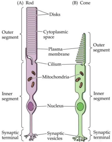
Figure 1.4The structure of a single rod (A) and cone (B) photoreceptor from the adult human retina. The outer segment (OS) of a photoreceptor houses the machinery necessary to detect light. The inner segment (IS) is responsible for the production of energy and metabolites that will be shipped to the outer segment. The cell body is responsible for mediating cell function, and synaptic terminals are responsible for carrying the signal to the innervated bipolar cells. (Image from the web site http://www.rci.rutgers.edu/~uzwiak/AnatPhys/Vision.htm)
9 The photoreceptors (Figure 1.4) are the sensors of the visual system that convert the capture of photons into a nerve signal in a process called phototransduction. The human retina contains approximately four to five million cones and 77–107 million rods. Only cones are found in the foveola, whereas rods predominate outside the foveola in the remaining fovea and all of the peripheral retina. Each photoreceptor consists of an outer segment (photopigment), inner segment (mitochondria, endoplasmatic reticulum), a nucleus, an inner fiber (analogous to an axon), and the synaptic terminal. The outer segment contains the photon-capturing photopigment. Opsin is a transmembranous protein that anchors the photopigment in the plasma membrane. In the outer segments, the plasma membrane is stacked into hundreds of flat discs, thereby increasing the density of retinal-opsin photopigment per photoreceptor cell. The discs in cones are deep invaginations of the outer segment membrane, while in rods, the discs are separate from the outer segment (except at the base). Shed discs are phagocytosed by the RPE. A nonmotile cilium connects the outer and inner segments. The inner segment contains the cellular machinery necessary to meet the high metabolic requirements of the photoreceptor cells. Its outer portion (the ellipsoid) is packed with mitochondria that produce ATP by oxidative phosphorylation, while the inner portion (the myoid) contains smooth and rough endoplasmic reticulum for synthetic activity as well as microtubules for intracellular transport. The photoreceptor nucleus contains all nonmitochondrial DNA. The inner fiber is the axon of the photoreceptor cell and transmits the photoreceptor cell signals to the outer plexiform layer (OPL) via its synaptic terminals. Due to the absence of inner nuclear layer cells in the foveola, foveolar inner fibers have to travel to the OPL in the surrounding macula to make synaptic contact. The synaptic neurotransmitter of the photoreceptor cell is glutamate, which is released in response to depolarization. The terminal endings of the photoreceptors interact with neighboring photoreceptors and interneurons (horizontal and bipolar cells) and play a critical physiological role in the transmission and early processing of visual information in the retina [2].
1.3 Phototransduction
In most sensory systems, activation of a receptor by the appropriate stimulus causes the cell membrane to depolarize, ultimately stimulating an action potential and transmitter release onto the neurons it contacts. In the retina, however, photoreceptors do not exhibit action
10 potentials; rather, light activation causes a graded change in membrane potential and a corresponding change in the rate of transmitter release onto postsynaptic neurons. Indeed, much of the processing within the retina is mediated by graded potentials, largely because action potentials are not required to transmit information over the relatively short distances involved.
Figure 1.5 An intracellular recording from a single cone stimulated with different amounts of
light (the cone has been taken from the turtle retina, which accounts for the relatively long time course of the response). Each trace represents the response to a brief flash that was varied in intensity. At the highest light levels, the response amplitude saturates (at about -65 mV). The hyperpolarizing response is characteristic of vertebrate photoreceptors; interestingly, some invertebrate photoreceptors depolarize in response to light [6].
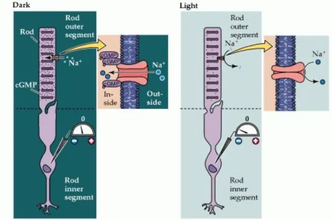
Perhaps even more surprising is that shining light on a photoreceptor, either a rod or a cone, leads to membrane hyperpolarization rather than depolarization (Figure 1.5). In the dark, the receptor is in a depolarized state, with a membrane potential of roughly -40 mV (including those portions of the cell that release transmitters). Progressive increases in the intensity of illumination cause the potential across the receptor membrane to become more negative, a response that saturates when the membrane potential reaches about -65 mV. Although the sign of the potential change may seem odd, the only logical requirement for subsequent visual processing is a consistent relationship between luminance changes and the rate of transmitter release from the photoreceptor terminals. As in other nerve cells, transmitter release from the synaptic terminals of the photoreceptor is dependent on voltage-sensitive Ca2+ channels in the terminal membrane. Thus, in the dark, when photoreceptors are relatively depolarized, the number of open Ca2+ channels in the synaptic terminal is high, and the rate of transmitter release is correspondingly great; in the light, when receptors are hyperpolarized, the number of open Ca2+ channels is reduced, and the rate of transmitter
11 release is also reduced. The reason for this unusual arrangement compared to other sensory receptor cells is not known.
The relatively depolarized state of photoreceptors in the dark depends on the presence of ion channels in the outer segment membrane that permit Na+ and Ca2+ ions to flow into the cell, thus reducing the degree of inside negativity (Figure 1.6). The probability of these channels in the outer segment being open or closed is regulated in turn by the levels of the nucleotide cyclic guanosine monophosphate (cGMP). In darkness, high levels of cGMP in the outer segment keep the channels open. In the light, however, cGMP levels drop and some of the channels close, leading to hyperpolarization of the outer segment membrane, and ultimately the reduction of transmitter release at the photoreceptor synapse.
Figure 1.6. Cyclic GMP-gated channels in the outer segment membrane are responsible for the light-induced changes in the electrical activity of photoreceptors (a rod is shown here, but the same scheme applies to cones). In the dark, cGMP levels in the outer segment are high; this molecule binds to the Na+-permeable channels in the membrane, keeping them open and allowing sodium (and other cations) to enter, thus depolarizing the cell. Exposure to light leads to a decrease in cGMP levels, a closing of the channels, and receptor hyperpolarization. (Image from the web site http://www.rci.rutgers.edu/~uzwiak/AnatPhys/Vision.htm)
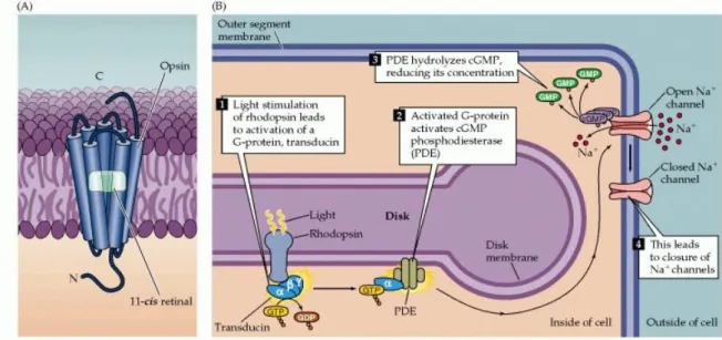
The series of biochemical changes that ultimately leads to a reduction in cGMP levels begins when a photon is absorbed by the photopigment in the receptor disks. The photopigment contains a light-absorbing chromophore (retinal, an aldehyde of vitamin A) coupled to one
12 of several possible proteins called opsins that tune the molecule's absorption of light to a particular region of the spectrum. Indeed, it is the different protein component of the photopigment in rods and cones that contributes to the functional specialization of these two receptor types. Most of what is known about the molecular events of phototransduction has been gleaned from experiments in rods, in which the photopigment is rhodopsin (Figure 1.7A); however, there is evidence that much of the inactivation process is paralleled in cones [7,8,9].
When the retinal moiety in the rhodopsin molecule absorbs a photon, its configuration changes from the 11-cis isomer to all-trans retinal; this change then triggers a series of alterations in the protein component of the molecule (Figure 1.7B). The changes lead, in turn, to the activation of an intracellular messenger called transducin, which activates a phosphodiesterase that hydrolyzes cGMP. All of these events take place within the disk membrane. The hydrolysis by phosphodiesterase at the disk membrane lowers the concentration of cGMP throughout the outer segment, and thus reduces the number of cGMP molecules that are available for binding to the channels in the surface of the outer segment membrane, leading to channel closure.
Figure 1.7. Details of phototransduction in rod photoreceptors. (A) The molecular structure of rhodopsin, the pigment in rods. (B) The second messenger cascade of phototransduction. Light stimulation of rhodopsin in the receptor disks leads to the activation of a G-protein (transducin), which in turn activates a phosphodiesterase (PDE). The phosphodiesterase hydrolyzes cGMP, reducing its concentration in the outer segment and leading to the closure of sodium channels in the
outer segment membrane. (Image from the web site
13 One of the important features of this complex biochemical cascade initiated by photon capture is that it provides enormous signal amplification. It has been estimated that a single light-activated rhodopsin molecule can activate 800 transducin molecules, roughly eight percent of the molecules on the disk surface. Although each transducin molecule activates only one phosphodiesterase molecule, each of these is in turn capable of catalyzing the breakdown of as many as six cGMP molecules. As a result, the absorption of a single photon by a rhodopsin molecule results in the closure of approximately 200 ion channels, or about 2% of the number of channels in each rod that are open in the dark. This number of channel closures causes a net change in the membrane potential of about 1 mV.
Equally important is the fact that the magnitude of this amplification varies with the prevailing levels of illumination, a phenomenon known as light adaptation. At low levels of illumination, photoreceptors are the most sensitive to light. As levels of illumination increase, sensitivity decreases, preventing the receptors from saturating and thereby greatly extending the range of light intensities over which they operate. The concentration of Ca2+ in the outer segment appears to play a key role in the light-induced modulation of photoreceptor sensitivity. The cGMP-gated channels in the outer segment are permeable to both Na+ and Ca2+; thus, light-induced closure of these channels leads to a net decrease in the internal Ca2+ concentration. This decrease triggers a number of changes in the phototransduction cascade, all of which tend to reduce the sensitivity of the receptor to light. For example, the decrease in Ca2+ increases the activity of guanylate cyclase, the cGMP synthesizing enzyme, leading to an increase in cGMP levels. Likewise, the decrease in Ca2+ increases the affinity of the cGMP-gated channels for cGMP, reducing the impact of the light-induced reduction of cGMP levels. The regulatory effects of Ca2+ on the phototransduction cascade are only one part of the mechanism that adapts retinal sensitivity to background levels of illumination; another important contribution comes from neural interactions between horizontal cells and photoreceptor terminals.
Once initiated, additional mechanisms limit the duration of this amplifying cascade and restore the various molecules to their inactivated states. The protein arrestin, for instance, blocks the ability of activated rhodopsin to activate transducin, and facilitates the breakdown of activated rhodopsin. The all-trans retinal then dissociates from the opsin, diffuses into the cytosol of the outer segment, and is transported out of the outer segment and into the pigment epithelium, where appropriate enzymes ultimately convert it to 11-cis retinal. After it is transported back into the outer segment, the 11-cis retinal recombines with opsin in the receptor disks. The recycling of rhodopsin is critically important for maintaining the light sensitivity of photoreceptors. Even under intense levels of illumination, the rate of
14 regeneration is sufficient to maintain a significant number of active photopigment molecules [10].
1.4 The Optical System of the Human Eye
As seen, the human eye functions as an optical system and consists of three main components: the cornea, the crystalline lens and in between them the iris. The cornea, the outermost optical element, is responsible for about 2/3 of the optical power and aberrations of the eye. The iris controls the amount of light coming into the retina by regulating the pupil diameter. The pupil has important consequences for image formation: a smaller pupil increases the depth of focus and minimizes the effects of high-order aberrations, on the contrary, the magnitude of aberrations increases with pupil dilation leading to a decrease in both visual performance and optical quality of the retinal image [1].
The crystalline lens accounts for about 1/3 of the optical power of the eye but it is capable of changing its focusing properties: controlled changes in the shape and thickness of the crystalline lens allow the eye to accommodate, the process by which the eye focuses on near objects.
Even in the normal eye, the optics and how they are aligned are not perfect, with the consequence that incoming light rays deviate from the desired path that reaches the foveal center. The deviations are defined as optical aberrations and can be classified into low-order (LOA) and high-order aberrations (HOA). LOA are the predominant optical aberrations, 90% of the overall wavefront aberration (WA) of the eye, and include defocus (hyperopia and myopia), the dominant aberration, followed by astigmatism. It is well known that HOA cannot yet be accurately corrected and greatly diminish the overall optical quality of the eye, though their contribution to the overall WA of the eye is ≤10% [11,12].
Aberrations impair ocular vision by bluring images formed on the retina, and decrease the quality in images taken of the retina by ophthalmic imaging cameras. To significantly improve visual performance and retinal imaging the eye's WA have to be measure and correct.
The presence of HOA, beyond defocus and astigmatism, has been known by researchers since the 19th century, but only in the 1990s wavefront sensors have been developed to allow routine estimation of the eye's WA.
15 Adaptive optics (AO) is a technology used to improve the performance of optical systems by minimizing aberrations. An AO ophthalmic device measures and corrects for the fluctuations of the eye’s WA, with improvement of the resolution of images taken from the eye. This technology has been developed for astronomical telescopes to remove the effect of atmospheric turbulence from astrophysics objects and only in recent years has been extended to ophthalmology [13,14]. By correcting ocular aberrations, AO retinal imaging can improve the resolution to 2 μm, providing information about the retinal microstructures not allowed with current retinal imaging techniques. Retinal imaging with AO technology represents a sensitive and accurate diagnostic tool to support the ophthalmologists in the diagnosis of retinal diseases at an early stage, and in the monitoring of the effects of new therapeutic treatments at microscopic scale.
1.5 Adaptive Optics Technology for Retinal Imaging
In the late 1990s, the principles and technologies of adaptive optics (AO), originally developed for astronomy, were adapted to image the retina. The history of adaptive optics for ophthalmic imaging is just over 20 years old. Adaptive optics by itself does not provide a retinal image, rather an AO subsystem must be incorporated into an imaging device. In 1989, Dreher et al. usedAO for the correction of second order optical aberrations of the eye [15]. Only in 1997, AO technology was successfully applied to high resolution imaging in the human eye by Liang et al. [16]. Since that time AO technology has been incorporated in almost all existing ophthalmic modalities to enhance quality and resolution of the retinal images: flood illumination fundus imaging, confocal scanning laser ophthalmoscopy and ophthalmic optical coherence tomography.
A typical AO retinal imaging camera has three principal components: a wavefront sensor, a corrective element and a control system, Figure 1.8. The wavefront sensor and corrector measure and correct the eye's wave aberrations respectively.
The wavefront sensor is used to measure the structure of the aberrations of the eye, with the Shack-Hartmann design being the most commonly used type. It consists of an array of lenslets, where each lenslet samples a local portion of the incident wavefront and focuses this light on a charge-coupled device (CCD). The displacement of any given spot from its intended position is directly related to the slope and amplitude of the wavefront in that portion of the pupil.
16 The corrective element (the “adaptive” optical element) is used to compensate for these aberrations, most commonly by using a deformable mirror, which relies on a series of actuators to deflect the mirror surface. There are many types of deformable mirrors in use in AO retinal imaging systems [14].
The AO controller, programmed with a computer, controls the interaction between the wavefront sensor and the corrector element; it interprets the wavefront sensor data and computes the appropriate wavefront corrector drive signals.
Figure 1.8. Basic layout of an adaptive optics system for retinal imaging. The system measures the ocular aberrations with a wavefront sensor and corrects for them with a wavefront corrector to achieve high lateral resolution imaging. Two light sources are generally used by an AO system: one is used to measure and correct the wavefront aberration of the eye; the second source is used to illuminate the retinal field being imaged. The AO compensated retinal image is captured by a high-resolution imaging camera [1].
AO systems operating in closed-loop place the wavefront sensor after the wavefront corrector. In this configuration, the measured wavefront is the error signal that gets fed back to the controller to further reduce the residual aberrations in the next iteration, theoretically correcting the retinal images up to the diffraction limit.
17
1.6 rtx1; Adaptive Optics Retinal Camera
In this work, the sequences of retinal images are obtained using a commercial AO-assisted flood illumination system; the rtx1 from Imagine Eyes, France as shown in Figure 1.9 [17, 18].
Figure 1.9 Rtx1 AO retinal camera by Imagine Eyes, France, (image from http://www.imagine-eyes.com/imagine-eyes-many-thanks-to-presenters-at-the-rtx1-e-workshop/).
The rtx1 has seven different optical paths; 4 for illumination, 1 for analysis and 2 for imaging. The illumination and imaging system of rtx1 are shown in Figures 1.10 and 1.11 respectively.
Figure 1.10 Illumination system of the rtx1 retinal camera (where r is retina, p is pupil, L is lenses, badal optometer, BS is the beam splitters, R-IL is the illumination source for the retinal imaging, FIX is the fixation target and A-IL is the illumination source for wavefront sensing) [18].
18
Figure 1.11 Imaging system of the rtx1 retinal camera (where r is retina, p is pupil, L is lenses, Badal optometer, DM is the deformable mirror, CCD is the scientific camera for retinal imaging, BS is beam splitters and sensor is the wavefront sensor) [18].
In the rtx1 retinal imaging illumination system, to provide a uniform illumination field on the retina an 850 nm LED (R-IL) is used. By a 750 nm super luminescent diode (SLD) (A-IL), a point source on the retina, for wavefront sensing, is created, and an array of ten 950 nm LEDs are used to uniformly illuminate the iris. As a fixation target on the retina, an internal organic light emitting diode (OLED) miniature monitor (FIX) is used.
In the rtx1 retinal imaging system, a low noise CCD camera (R-CCD) (Rooper Scientific) with 1392 x 1040 pixels is used to image the 4°x 4° area of the retina, which corresponds to approximately 1.2 mm x 1.2 mm in the retina for an emmetropic eye. Here, one camera pixel is equivalent to 1.6 µm in the retina. The rtx1 uses a continuous magnetic deformable mirror mirao52e (Imagine Eyes, France) which provides a maximum ±50 µm stroke to correct for the aberrations present in almost any eye. In this deformable mirror, the magnets are glued under the continuous membrane of the mirror and set above coils. When voltage is applied to the coils, they generate magnetic fields which push or pull the magnets. Here, the 52 actuators are placed in an ~ 17 mm diameter area where the mirror surface covers an area of 15 mm diameter.
The pupil imaging used for patient alignment is using a standard CCD (Allied vision) camera with 656 x 494 pixels mounted with a standard objective (Pentax) with a focal length of 35 mm. In addition, each of the optical paths except for pupil illumination and imaging, has a badal system to compensate for the eye ametropia from -10 D to + 8 D, leaving the deformable mirror stroke fully available to compensate for astigmatism up to 5D, strong eye optical defects and to focus the image at different layers of the retinal microstructure. The rtx1 imaging system requires 9 ms exposure time. The total acquisition time for the 40 frames is approximately 4 seconds with 105 ms of interval time between the frames [18].
19 The full exam including patient alignment and post-processing takes a few minutes per eye for most patients, making it suitable for use in large-scale clinical studies.
The AO retinal camera, rtx1, allows to resolve numerous structural aspects of the living human retina by the direct visualization of photoreceptors, retinal vessels and nerve fiber bundles. The photoreceptor cells represent the study primary target for many research groups. Due in part to the optical waveguide properties of photoreceptors, the cone mosaic can be imaged easily (Figure 1.12), and furthermore, many retinal diseases involve cones losses.
Figure 1.12. Example of rtx1 AO image montage form a healthy 29 year old female subject.
1.7 The Photoreceptor Mosaic and degenerative diseases of the
human retina
The arrangement of the photoreceptor types in the retina is well described histologically [19,20]. The cone and rod photoreceptors are closely packed, forming a patterned appearance, or mosaic. Rods substantially outnumber cones over the entire retina. In the
20 developing human retina, the relative distribution of cone and rod photoreceptors is roughly constant; that is, a 20:1 ratio is maintained across the entire retina. However, across an adult retina, the ratio of rods to cones varies substantially. The adult fovea contains the highest density of cone photoreceptors, enabling high acuity vision.
However, the density of cone photoreceptors quickly falls off as a function of distance from the fovea, yielding to a high density of rod photoreceptors, which peaks at about 10 degrees from the fovea (Figure 1.13).
Figure 1.13 Rods (in violet) and cones (in green) are distributed regionally: in the Center of the eye (i.e., the fovea) there are only cones; in the Peripheral retina, mainly rods and few cones. (Image from the web site http://www.rci.rutgers.edu/~uzwiak/AnatPhys/Vision.htm)
In some eye diseases, the retina becomes damaged or compromised, and degenerative changes set in that eventually lead to serious damage to the nerve cells that carry the vital messages about the visual image to the brain. Many inherited and acquired retinal diseases are associated with disruption or alteration of photoreceptor structure and function, including Best vitelliform macular dystrophy, retinitis pigmentosa, Usher syndrome, cone-rod dystrophy, age-related macular degeneration, and diabetic retinopathy (Figure 1.14).
21 Figure 1.14 A view of the fundus of the eye and of the retina in patients who have
acquired and inherited retinal diseases [21].
These pathologies are typically tracked using clinical instruments which have resolution limited to gross retinal structures, thereby limiting the ability to effectively track disease progression at cellular level.
Adaptive optics (AO) ophthalmoscopy can be applied to assess these pathologies with very high resolution, allowing a finer view of retinal disease progression [22], Figure 1.15.
Figure 1.15. Adaptive optics images of the parafoveal cone mosaic in patients with retinal diseases and healthy subjects acquired at 1.5 degrees superior from the fovea. Up: the photoreceptor mosaic showed variable cell loss and abnormalities in the packing arrangement of the cones with respect to healthy subjects (down).
22
1.8 Summary of dissertation aim
The assessment of the structure of the photoreceptor mosaic in AO images needs methods to quantify the arrangement of the cells. For this purpose, a variety of geometric and statistical algorithms were developed to analyse the coordinates identifying the position of cone centroids. In particular, the most used metrics are cell density, the percentage of six-sided Voronoi cells and spacing metrics.
The aim of this thesis is to study the arrangement of the parafoveal cone mosaic from AO flood illumination images with two different approaches:
1. The first approach is a global analysis of the spacing between cones by extraction of three frequently used spacing metrics;
2. The second approach is a local pointwise analysis of the tendencies of the cones for aggregation and repulsion at specific distance, by statistical point pattern analysis.
First, Chapter 2 explores the relationship between in-use spacing metrics of photoreceptor structure and how each is affected by changes in retinal eccentricity and window sample size. This chapter deals with the introduction and the assessment of three spacing metrics, the center-to-center spacing (Scc), the local cone spacing (LCS), and the Density Recovery Profile Distance (DRPD) frequently used to evaluate the distribution of cell distances in adaptive optics (AO) images of the cone mosaic.
Chapters 3 focus on the application of new approaches for measuring photoreceptor arrangement by spatial point pattern analysis. Here we used statistical second order descriptors to characterize the spatial distributions of photoreceptors in real and simulated images. These spatial descriptors include the pair correlation function g2(r), the structure factor s(k) and various nearest neighbor second order statistics (G(r), K(r) and L(r)), to quantify the reciprocal influence of the cells at a variable distance r.
Finally, starting from the results of the previous spatial point pattern analysis, the aim of Chapter 4 is evaluating dissimilarities profiles of the individual spatial second order functions, seen in the previous chapter 3, extracted from the control and diseased groups, for partitioning individual curves into homogeneous classes.
23
Chapter 2
Reliability and agreement between metrics of cone spacing in
adaptive optics images of the human retinal photoreceptor
mosaic
24
2.1
Introduction
Adaptive optics (AO) retinal imaging has enabled direct visualization of the cone mosaic and measurement of density, spacing and packing arrangement of cones in normal eyes and eyes with retinal diseases [23,24]. Since an increasing number of studies is providing descriptive information about the integrity and pathological change of the retinal cone mosaic using various approaches, it is of clinical importance to understand whether the results from different studies can be reliably compared [25,29]. In previous work [30,31], we have evaluated the agreement of density and packing arrangement of cones between sampling areas of different size and geometry. The results from normal eyes have shown that caution is needed when comparing cone density evaluated in sampling areas of different sizes (the average difference can reach 10% between 320x320 µm and 64x64 µm sampling windows) [30,31];the packing arrangement of cones by Voronoi analysis has been shown to be minimally affected by window size. To construct a Voronoi, each cone, identified by its geometrical centroid, corresponds to a Voronoi tile that is color coded with respect to their cones neighbors. The primary advantages and drawbacks of these metrics have been previously discussed [1,26,27,30,31]. Cone density analysis creates strict demands on image quality because it requires that all cones within the region of interest be identified. For this reason, manual inspection of the cones in each image is highly recommended in order to minimize errors [1,26,30,31]. In addition, the moderate to high variability of cone density even in healthy adults may make this metric insensitive to small deviations from normal [1,29]. The limit of Voronoi analysis is related to the accuracy of the cone identification algorithm, the manual re-selection of the unidentified or misidentified cones, and the boundary effect which is an apparent distortion of the Voronoi mosaic due to the exclusion of cones beyond the sampling window, the effect of which increases as the sampling window decreases [30,31]. It has been previously shown that the cone detection algorithm which segments the cone aperture, rather than only identifying the cone centroid position, is the most accurate approach for identifying the cones [32,33].
Despite broad use of spacing metrics in clinical studies, there have been few evaluations of the reliability and agreement among various metrics.13 Overall, cone spacing analysis is less affected by image quality variations than cone density, because these methods do not require identification of every cone within the region of interest [1,25,26,28,35]. For this reason, spacing metrics can be less prone to errors than cone density when tracking disease progression or response to treatment in eyes with retinal diseases, in which cones may be poorly imaged due to loss of wave-guiding property or missing cells [25]. However, there is
25 no supporting evidence that cone spacing metrics alone may provide a robust measurement for comparison among eyes (or even the same eye over time) in clinical studies [1,25,34,35]. The majority of studies have used two main methodologies to estimate the spacing of cells in AO images of the cone mosaic; the density-count method and the distribution-of-distances methods. The center-to-center spacing (Scc) is a measure that has been frequently adopted in studies of cone photoreceptor mosaic [36,37,38].The Scc is based on the density count method, which is derived from the number of cones per unit area. The distribution-of-distances methods are assumption free and provide estimates of both central tendency and variation. These methods include the nearest neighbour distance (NND), the local cone spacing (LCS), and the nearest-neighbour cone spacing extracted from the Density Recovery Profile (DRP), which has been recently termed Density Recovery Profile Distance (DRPD) [19,34,39,40].
The scope of the present work was to assess the reliability and agreement of three spacing metrics, such as Scc, LCS and DRPD, for evaluating the distribution of cell distances in AO flood illumination images of the parafoveal cone mosaic. The metrics were calculated over two different sampling areas to evaluate the effect of window size on cone spacing estimates. In order to evaluate the influence of cell reflectivity loss and cone packing arrangement abnormalities on spacing metrics, the dataset included AO images acquired from healthy adult subjects and patients with a diagnosis of acquired or inherited retinal diseases.
2.2
Methods
All research procedures described in this work adhered to the tenets of the Declaration of Helsinki. The protocol was approved by the local ethical committee (Azienda Sanitaria Locale Roma A, Rome, Italy) and all subjects recruited gave written informed consent after a full explanation of the procedure. Inclusion criteria were age >18 years old, no previous eye surgery, eye inflammation, glaucoma or cataract; in addition, control subjects were required to have no history or presence of systemic diseases. Subjects recruited for the study received a complete eye examination, including non-contact ocular biometry using the IOL Master (Carl Zeiss Meditec Inc, Jena, Germany).
26
2.2.1
Human subjects
Twenty healthy volunteers (age 33± 9 years old; range 23-54 years; gender: 15 F and 5 M), and twelve patients with retinal diseases (age 41±10 years old; range 23-59 years; gender: 10 F and 2 M) were recruited in this study (Table 2.1). The latter participants included subjects with a diagnosis of diffuse cuticular drusen and a family history of age-related macular degeneration (Drusen; n=2) [41,42], non proliferative diabetic retinopathy (NPDR;
Table 2.1. Characteristics of study participants.
Participants Age (years) Gender AxL (mm)* SEr (D)* RMFcorr (mm/deg2)* Healthy subjects C_1 52 F 24.73 -0.5 0.294 C_2 37 F 25.49 -4.7 0.303 C_3 24 F 25.06 -2.7 0.298 C_4 32 M 27.04 -6.2 0.322 C_5 33 F 23.60 0.0 0.281 C_6 27 M 23.58 -2.5 0.281 C_7 40 M 22.61 0.0 0.269 C_8 26 F 26.29 -5.2 0.313 C_9 24 F 21.66 -1.2 0.258 C_10 36 F 25.67 -5.2 0.306 C_11 39 F 22.11 0.2 0.263 C_12 37 F 22.11 0.5 0.263 C_13 29 F 24.42 -2.2 0.291 C_14 24 F 24.38 -3.7 0.290 C_15 23 F 25.34 -3.5 0.302 C_16 36 F 23.98 -5.1 0.285 C_17 54 F 24.73 -0.5 0.294 C_18 23 F 24.53 0.0 0.292 C_19 46 M 23.50 0.2 0.280 C_20 33 M 23.69 0.0 0.282 M±SD 33 ± 9 24.23±1.42 -2.1±2.3 0.200±0.017 Retinal diseases Drusen_1 38 M 24.03 -0.2 0.286 Drusen_2 42 F 25.40 -0.5 0.302 NPDR_1 51 F 24.77 -1.5 0.295 NPDR_2 38 F 23.80 0.0 0.283 NPDR_4 33 M 26.34 -4.2 0.314 NPDR_5 35 F 21.89 0.0 0.261 Best 56 F 24.07 -0.5 0.286 OMD 23 F 25.57 -2.0 0.304 RP_1 46 F 24.50 -1.0 0.292 RP_2 40 F 23.20 0.0 0.276 RP_3 42 F 22.62 1.0 0.269 RP_4 59 F 22.81 1.0 0.271 M±SD 41± 10 24.08±1.32 -0.7±1.4 0.287±0.016
27 n=4) according to the ETDRS severity scale [43,44], retinitis pigmentosa (RP; n=4; USH2A gene mutation), Best macular dystrophy (Best; n=1; BEST 1 gene mutation) and occult macular dystrophy (OMD; n=1; RP1L1 gene mutation) [45].
These participants were enrolled in this study in order to have a dataset of AO images of the cone mosaic with increasing amount of cell loss and variable abnormalities in the packing arrangement of the cones.
2.2.2
Image acquisition and processing
A flood-illuminated AO retinal camera (rtx1, Imagine Eyes, France) was used to collect images of the cone mosaic on 20 healthy subjects and 12 subjects with various retinal diseases. The imaging session was conducted after dilating the pupil with one drop of 1% tropicamide. During imaging, fixation was maintained by instructing the patient to fixate on the internal target of the instrument moved by the investigator. At each retinal location, a sequence of 40 frames (rate: 9.5 frames/sec) was acquired by illuminating a retinal area subtending 4 degrees of visual angle in the right eye of each subject; images were acquired at several locations in the central retina covering an area of 5x4 degrees centered on the preferred locus of fixation (PRL, coordinates x=0° and y=0° and here used as the foveal reference point).
A proprietary program from the manufacturer has been used to correct for distortions within frames of the raw image sequence and to register and frame-average to produce a final image with enhanced signal-to-noise ratio prior to further analysis. In this study, two sampling areas of different size (64x64 µm and 204x204 µm) were cropped from each final image at 1.5 degrees superior and 2.5 degrees temporal from the PRL. The two eccentricities were chosen to be a compromise between the resolution limit of the instrument, which does not allow all the cones to be resolved too close to the fovea, and the presence of rods, which alter the cone relative spacing enough to be detectable by the instrument when further than 4 degrees from the fovea.
The nonlinear formula of Drasdo and Fowler and the Gullstrand schematic model eye parameterized by the biometry measurements (corneal central curvature, anterior chamber central depth, axial length) were used to convert each final image from degrees of visual angle to micrometers on the retina [46,47]. The corrected magnification factor (RMFcorr) was calculated for each eye in order to correct for the differences in optical magnification and thus retinal image size between eyes, as previously described [30,31,44-47].
28 Image cone labelling was automatically performed using an enhanced version of the algorithm implemented with the image processing toolbox in Matlab (The Mathworks Inc, Natick MA, USA) [30,31,43,44,48].Cones were identified independently in each sampling window. The cone identification algorithm’s performance was verified by three expert investigators (DG, LM, ML), who reviewed each sampling area and manually identified cones that they agreed to be missed or selected in error by the algorithm. This procedure ensured that the number of excluded cones was minimised. A buffer zone was created in each sampling window in order to minimize the boundary effect for packing geometry metrics [30.31]. The x,y coordinates of the cones in each sampling window were then stored in a text array and used to calculate the cone metrics.
2.2.3
Density and packing arrangement metrics of the cone mosaic
Cone counts were converted into local densities by calculating their number per square millimeter (cones/mm2). The cone packing arrangement was analyzed using Voronoi diagrams [30,31,49,50]. The Voronoi tessellation was implemented by the voronoi Matlab function from the bidimensional coordinates of labelled cones, as previously described [30,31,44,49].The Voronoi regions lying at the bounds of each section were excluded from further analysis, creating a buffer zone = 2 NND in order to minimize the boundary effect. The number of Voronoi tiles with six sides (6n) was divided by the total number of bound Voronoi tiles within each sampling area and expressed as a percentage.
2.2.4
Spacing metrics of the cone mosaic
Three metrics were used to describe the distribution of cone distances:
1. The center-to-center spacing (Scc) was determined from cone density using the following expression: 2 / 1 3 2 1000 D Scc (2.1)
where D is the number of cones per square millimeter. Since the method assumes an exact relationship between cone density and spacing, the cones are expected to be arranged in triangular lattice (this metric was also termed minimum center-to-center
29 spacing) [36-38,49]. It is equivalent to the metric S used by Chui et al. [36]and S(x,y) used by Li et al. [37]. Care should be taken to avoid regions of missing data (e.g., large blood vessels, image boundary etc.) or defects in the image in order to avoid overestimating the spacing distribution of cones.
2. The local cone spacing (LCS) was determined by calculating the average of the minimum distances from the center of a given cone to the centers of six neighboring cones within an area of 12 pixels (9.6 µm) diameter (i.e., almost twice the size of the cone at both retinal locations) [44]. The LCS has been developed in order to minimize the known limits of NND in estimating the mosaic spacing. Indeed, the NND takes into account only the nearest of each cell’s known neighbours, regardless of its distance; therefore, it can be strongly influenced by very large NNDs of isolated cells, which decrease its sensitivity to represent the distribution of cell distances in retinal diseases [34].
3. The density recovery profile distance (DRPD) was derived from the DRP reconstructed from the autocorrelogram [39]. The spatial autocorrelogram was generated by superimposing the distribution of all cells in a sampling area using each cell in the area in turn as the reference cell. In order to determine the nearest-neighbour cone distance, the DRPD was calculated as the first local maximum of the Density Recovery Profile created from the autocorrelogram with max radius = 1/5 of the image dimension and a series of annuli of 1 µm width. The width of each bin was determined from equation 16 in Rodieck et al. [39], under assumption of having a reliability factor value of 5 and 4 for healthy subjects and patients with retinal diseases, respectively. The bin’s width was accordingly 1 µm in the two populations. The DRPD takes into account all of a cell’s neighbours up to a limited distance that depends on the shape of the DRP, which is a graphical representation of spatial behaviour derived from the spatial autocorrelogram [39]. It is equivalent to the nearest-neighbour cone spacing determined from the DRP in previous studies [25,35]. Nevertheless, the DRP provides a different measure than the nearest neighbour distance and a more complete overview of the spatial arrangement of the cone mosaic; its estimates are based upon all of the other points about a given point, rather than just one.
30
Figure 2.1 - Adaptive optics images of the parafoveal cone mosaic in patients with retinal diseases and healthy
subjects acquired at 1.5 degrees superior and 2.5 degrees temporal from the fovea. The photoreceptor mosaic in patients with retinal diseases showed variable cell loss and abnormalities in the packing arrangement of the cones with respect to healthy subjects. The sampling area subtends 64x64 μm. Data from participants are summarized in table 2.1.
Figure 2.2 - Adaptive optics images of the parafoveal cone mosaic in patients with retinal diseases and healthy
subjects acquired at 1.5 degrees superior and 2.5 degrees temporal from the fovea. The sampling area subtends 204x204 μm. Data from participants are summarized in table 2.1.
31
2.2.5
Statistics
Data were expressed as mean ± standard deviation. Statistics were performed using the SPSS software (version 17.1; SPSS Inc., Chicago, IL USA) and Matlab (version R2013a, The Mathworks Inc., Natick MA, USA).
The sample size was calculated to detect a mean difference in cone density of 2500 cones/mm2 (SD = 2500 cones/mm2) between healthy subjects and patients with retinal diseases (2:1 allocation) with a two-sided significance level of 5% and a power of 82%. The intraclass correlation coefficient (ICC; two-way, random effects model) was calculated in order to estimate the absolute agreement between each pair of spacing metrics in the two sampling areas for each study group. The correlation and Bland-Altman analysis were used to assess the 95% limits of agreement (LoA) between the pair of spacing metrics that have shown high absolute agreement (ICC>0.7), and between the values of each spacing metric extracted from the two sampling areas. The differences between the spacing metrics of the two study groups was evaluated using the non-parametric Mann Whitney U test.
2.3
Results
2.3.1
Cone density and packing arrangement
Over a 64x64 µm sampling area, the cone densities at 1.5 degrees and 2.5 degrees retinal eccentricities in healthy subjects were 32281±2281 cones/mm2 and 29411±2147 cones/mm2, respectively (Figure 2.1). Cone density in patients with retinal diseases was on average 26±3% (range from 2% to 65%; P<0.001) lower than in healthy subjects.
Over a 204x204 µm sampling area, the cone densities at 1.5 degrees and 2.5 degrees from the PRL in healthy subjects were 31494±2489 cones/mm2 and 28703±1822 cones/mm2, respectively (Figure 2.2). Cone density in patients with retinal diseases was on average 16±5% (range from 1% to 58%; P<0.001) lower than that in healthy subjects.
The average percentage of six-sided Voronoi tiles was almost constant across different sampling areas in either study groups. In healthy subjects, the 6n Voronoi average ranged from 50% to 45% for 1.5 degrees and 2.5 degrees, respectively. In patients with retinal diseases, the average 6n Voronoi tiles were significantly lower than control values (P<0.05), except for values calculated in 204x204 µm sampling areas at 2.5 degrees retinal eccentricity (P=0.14). Cone density and percent of six-sided Voronois for all cases are shown in table 2.2.
32
Table 2.2. Mean (±SD) cone density and percentage of six-sided (6n) Voronois in study participants over different sampling areas at two retinal locations.
Sampling area 64 µm x 64 µm 204 µm x 204 µm
Metric Cone density (cones/mm2) 6n Voronois (%) Cone density (cones/mm2) 6n Voronois (%)
Retinal
eccentricity 1.5 degrees 2.5 degrees 1.5 degrees 2.5 degrees 1.5 degrees 2.5 degrees 1.5 degrees 2.5 degrees
Healthy subjects C_1 30476 26905 51.1 47.3 29924 27438 48.7 43.2 C_2 36341 30732 57.0 46.5 35517 30154 57.1 48.1 C_3 29286 26429 48.2 45.3 27683 26591 51.5 45.9 C_4 31951 28780 55.9 45.6 31707 28331 55.7 48.0 C_5 34146 33659 47.0 40.8 33397 32153 47.0 42.4 C_6 28537 30976 59.3 45.6 27632 29587 53.0 41.7 C_7 31951 29024 43.0 40.9 30431 27392 39.1 45.5 C_8 32927 28780 41.8 51.2 34880 27861 47.3 48.4 C_9 31220 28537 48.9 32.5 29021 27375 48.2 39.7 C_10 36098 30732 50.9 43.0 34641 29139 48.7 48.0 C_11 34146 28537 44.5 40.7 31599 27446 43.8 40.0 C_12 32195 26585 41.8 44.8 31367 29305 44.1 41.6 C_13 34878 29512 57.6 50.0 33861 27387 54.5 53.9 C_14 35366 27561 58.2 50.6 34053 26595 52.5 52.7 C_15 32927 27805 60.4 44.9 34378 27081 53.2 47.2 C_16 30488 30488 44.8 46.0 30571 30476 42.2 46.1 C_17 30000 29756 39.3 39.3 28490 28727 51.1 44.4 C_18 30000 34390 59.5 53.0 29333 32952 51.6 46.1 C_19 30732 27805 40.5 48.7 29986 27374 38.0 45.3 C_20 31951 31220 54.4 39.1 31411 30694 51.1 40.9 M±SD 32281±2281 29411±2147 50.3±7.0 44.8±4.9 31494±2489 28703±1822 48.9±5.3 45.5±3.9 Retinal diseases Drusen_1 24146 27317 48.5 44.2 22679 28900 50.1 43.4 Drusen_2 24390 28780 41.2 49.4 27524 28762 42.9 41.5 NPDR_1 26341 23902 39.2 34.4 26571 24000 47.5 47.9 NPDR_2 26098 23171 44.4 47.6 26738 23452 42.9 46.6 NPDR_4 31707 24146 34.8 47.7 32110 25396 47.9 46.4 NPDR_5 24146 25122 48.4 36.6 24442 23444 43.2 43.5 Best 23500 25750 58.1 34.8 25444 24412 45.6 48.8 OMD 11463 10244 44.0 31.8 13134 16914 35.5 33.4 RP_1 19024 17073 43.7 30.2 26754 27112 41.2 39.1 RP_2 24146 23902 47.6 35.9 25273 27411 39.1 41.7 RP_3 25366 21951 41.4 37.9 26850 25298 41.0 39.3 RP_4 19512 18293 32.6 34.7 25273 26247 41.7 41.3 M±SD 23320±4937 22471±5089 43.7±6.8 38.8±6.7 25233±4422 25112±3203 43.2±4.1 42.7±4.4 P value <0.001 <0.001 0.02 0.01 <0.001 <0.001 0.003 0.14
33
2.3.2
Cone spacing metrics
In healthy subjects, the values of all spacing metrics increased with increasing eccentricity and showed high consistency between the two different sampling areas; Scc ranged from 5.99±0.21 µm to 6.35±0.24 µm from 1.5 degrees to 2.5 degrees from the fovea respectively; LCS ranged from 6.12±0.18 µm to 6.41±0.18 µm respectively; and DRPD ranged from 5.80±0.80 µm to 6.20±0.66 µm respectively. In patients with retinal diseases, the spacing metrics showed higher variation around the mean values, which was caused by the abnormal and variable distribution of distances between cells across the parafoveal retinal locations in the disease population (Table 2.3).
The differences of Scc and LCS values between healthy subjects and patients with retinal diseases were statistically significant (P≤0.01) in both sampling areas at both retinal eccentricities, except for the LCS values measured in the 204x204 µm area at 2.5 degrees retinal eccentricity (P=0.27). This result was consistent with the distribution of 6n Voronois between healthy and pathologic cases in the same area (see Table 2.2). The differences of DRPD values between healthy subjects and patients with retinal diseases were not statistically significant in any case.
2.3.2.1 Agreement and correlation between spacing metrics
The Scc and LCS values showed high agreement with each other in healthy subjects over both sampling areas and both retinal eccentricities (averaged ICC=0.86; ICC range=0.80-0.93). On the other hand, the agreement between Scc and LCS values in patients with retinal diseases was poor (averaged ICC=0.28; ICC range=0.08-0.51). The agreement between the DRPD and the other two spacing metrics was low in both study groups (averaged ICC=0.27; ICC range=0.05-0.47). The ICC analysis between each pair of spacing metrics is summarized in Table 2.4.
34
Table 2.3. Mean (±SD) values of the three spacing metrics in different sampling areas at two retinal locations.
Sampling area 64 µm x 64 µm 204 µm x 204 µm Metric Scc (µm) LCS (µm) DRPD (µm) Scc (µm) LCS (µm) DRPD (µm) Retinal eccentricity 1.5 deg 2.5 deg 1.5 deg 2.5 deg 1.5 deg 2.5 deg 1.5 deg 2.5 deg 1.5 deg 2.5 deg 1.5 deg 2.5 deg Healthy subjects C_1 6.16 6.55 6.22 6.57 5.50 6.50 6.21 6.49 6.29 6.46 5.50 6.50 C_2 5.64 6.13 5.86 6.31 5.50 6.50 5.70 6.19 5.82 6.25 5.50 5.50 C_3 6.28 6.61 6.39 6.65 6.50 6.50 6.46 6.59 6.51 6.59 5.50 6.50 C_4 6.01 6.33 6.07 6.43 5.50 5.50 6.03 6.38 6.12 6.45 5.50 6.50 C_5 5.82 5.86 5.90 6.05 5.50 5.50 5.88 5.99 5.96 6.08 5.50 5.50 C_6 6.36 6.11 6.09 6.38 5.50 5.50 6.46 6.25 6.26 6.53 5.50 5.50 C_7 6.01 6.31 6.41 6.28 6.50 6.50 6.16 6.49 6.50 6.31 6.50 6.50 C_8 5.92 6.33 6.01 6.38 5.50 6.50 5.75 6.44 5.86 6.50 5.50 6.50 C_9 6.08 6.36 6.18 6.52 6.50 5.50 6.31 6.49 6.36 6.52 6.50 6.50 C_10 5.66 6.13 5.89 6.40 4.50 5.50 5.77 6.30 5.86 6.42 5.50 5.50 C_11 5.82 6.36 6.07 6.95 5.50 6.50 6.05 6.49 6.15 6.51 6.50 6.50 C_12 5.99 6.59 6.08 6.63 5.50 6.50 6.07 6.28 6.17 6.36 5.50 6.50 C_13 5.75 6.26 5.92 6.43 5.50 5.50 5.84 6.49 5.96 6.60 5.50 5.50 C_14 5.71 6.47 5.89 6.61 5.50 5.50 5.82 6.59 5.91 6.65 5.50 5.50 C_15 5.92 6.44 6.07 6.38 5.50 7.50 5.80 6.53 5.90 6.55 5.50 6.50 C_16 6.15 6.15 6.33 6.27 6.50 5.50 6.15 6.16 6.20 6.24 6.50 5.50 C_17 6.20 6.23 6.37 6.46 5.50 7.50 6.37 6.34 6.42 6.37 5.50 6.50 C_18 6.20 5.79 6.28 5.91 5.50 6.50 6.27 5.92 6.34 5.99 5.50 5.50 C_19 6.13 6.44 6.31 6.53 8.50 6.50 6.21 6.49 6.25 6.52 8.50 6.50 C_20 6.01 6.08 6.11 6.27 5.50 6.50 6.06 6.13 6.14 6.24 5.50 6.50 M±SD 5.99± 0.21 6.28± 0.22 6.12± 0.18 6.42± 0.22 5.80± 0.8 6.20± 0.66 6.07± 0.24 6.35± 0.19 6.15± 0.22 6.41± 0.18 5.85± 0.75 6.10± 0.5 Retinal diseases Drusen_1 6.92 6.50 6.91 6.57 5.50 5.50 7.14 6.32 7.01 6.32 6.50 5.50 Drusen_2 6.88 6.33 6.64 6.31 5.50 4.50 6.48 6.34 6.33 6.29 5.50 5.50 NPDR_1 6.62 6.95 6.55 6.82 6.50 6.50 6.59 6.94 6.59 6.83 5.50 6.50 NPDR_2 6.65 7.06 6.56 6.88 6.50 5.50 6.57 7.02 6.54 6.86 6.50 6.50 NPDR_4 6.03 6.92 6.08 6.81 5.50 6.50 6.00 6.74 6.02 6.73 5.50 6.50 NPDR_5 6.92 6.78 6.74 6.59 6.50 6.50 6.87 7.02 6.65 6.79 6.50 6.50 Best 7.01 6.70 6.94 6.61 6.50 6.50 6.74 6.88 6.67 6.70 6.50 6.50 OMD 10.04 10.62 6.91 6.48 6.50 4.50 9.38 8.26 6.59 6.38 6.50 4.50 RP_1 7.79 8.22 6.62 6.56 4.50 4.50 6.57 6.53 6.26 6.14 5.50 4.50 RP_2 6.92 6.95 6.69 6.34 6.50 4.50 6.76 6.49 6.47 6.34 5.50 5.50 RP_3 6.75 7.25 6.50 6.70 5.50 7.50 6.56 6.76 6.36 6.46 6.50 5.50 RP_4 7.69 7.95 6.60 6.61 5.50 4.50 6.76 6.63 6.44 6.46 5.50 5.50 M±SD 7.19± 1.01 7.35± 1.16 6.65± 0.23 6.61± 0.18 5.92± 0.67 5.58± 1.08 6.87± 0.84 6.83± 0.51 6.49± 0.25 6.53± 0.24 6.00± 0.52 5.75± 0.75 P value <0.001 <0.001 <0.001 0.01 0.32 0.09 <0.001 <0.001 <0.001 0.27 0.25 0.25
35 In healthy subjects, the correlation between Scc and LCS was high over both sampling areas (R2=0.75, P<0.001; and R2=0.88, P<0.001, over 64x64 µm and 204x24 µm respectively) (Figure 2.3). In patients with retinal diseases, the correlation between Scc and LCS was poor over both sampling areas (R2=0.018, P=0.53; and R2=0.25, P=0.014, respectively).
The 95% LoA was slightly influenced by window size; the agreement between Scc and LCS values over 204x204 µm areas was greater than 64x64 µm areas (Figure 2.3). This was associated with the greater percentage of 6n Voronois in patients with retinal diseases over a 204x204 µm sampling window.
Table 2.4. Intraclass correlation coefficient (ICC) showing, for each study group, the absolute agreement between cone spacing metrics in two different sampling areas at two retinal locations.
Sampling area 64 µm x 64 µm 204 µm x 204 µm
Retinal eccentricity 1.5 degrees 2.5 degrees 1.5 degrees 2.5 degrees
Healthy subjects
ICC between Scc and LCS* 0.80 0.80 0.93 0.93
ICC between Scc and DRPD 0.33 0.26 0.24 0.44
ICC between LCS and DRPD 0.37 0.11 0.25 0.25
Retinal diseases
ICC between Scc and LCS 0.08 0.23 0.51 0.29
ICC between Scc and DRPD 0.05 0.47 0.36 0.14
36
Figure 2.3 – A) Correlation between local cone spacing (LCS) and center -to-center spacing (Scc) in
64x64 µm sampling areas. Data were aggregated from 1.5 degrees and 2.5 degrees retinal eccentricities. In healthy subjects, the correlation between LCS and Scc was high (R2=0.75, y=0.846x+1.082,
P<0.001); almost all values (85%) were on the bisector ( y=x, R2=1). In patients with retinal diseases,
the correlation between LCS and Scc was very low (R2=0.018, y=-0.028x+6.733, P=0.53); the patients
with advanced stages of inherited retinal dystrophies (OMD and RP) and diffuse loss of cone reflectivity (≥30%) primarily contributed to the decreased correlation between this pair of spacing metrics. B) Correlation between LCS and Scc in 204x204 µm sampling areas. In healthy subjects, the correlation
was high (R2=0.89, y=0.859x+0.946, P<0.001); 95% of the LCS and S
cc values were on the bisector. In
patients with retinal diseases, correlation between LCS and Scc was low (R2=0.25, y=0.171x+5.433,
P=0.01). C and D) Bland-Altman plots of Scc and LCS values calculated over 64x64 μm and 204x204
μm sampling areas respectively. Although the agreement between this pair of spacing metrics was high in the 64x64 μm area, the use of greater sampling areas further increased agreement between metrics. The symbols are described in the plot.
2.3.2.2 Influence of the sampling area on Scc
The Scc values calculated over sampling areas of different sizes showed high correlation both in healthy subjects (R2=0.84, P<0.001) and patients with retinal diseases (R2=0.66, P<0.001). On the other hand, the distribution of data points in the Bland-Altman plot showed that agreement was poor for Scc values estimated from cone mosaics with more than 30% cone reflectivity loss (Figure 2.4).
37
Figure 2.4 –A) Correlation between Scc values calculated in the two sampling areas of 64x64 μm and
204x204 μm. In healthy subjects, the correlation was high (R2=0.84, y=0.924x+0.541, P<0.001), with
85% of Scc values that were on the bisector. In patients with retinal diseases, the correlation was
moderate (R2=0.67, y=0.517x+3.088, P<0.001); the patients with advanced stages of inherited retinal
dystrophies (OMD and RP) and diffuse loss of cone reflectivity (≥30%) contributed to decrease the overall correlation between Scc values taken over sampling areas of different sizes. B) Bland -Altman
plot of Scc values. The outliers in the Bland-Altman plot are represented by three patients (OMD, RP1
and RP4; see table 3.1) that had the lowest cone density in the study population. Data were aggregated from 1.5 degrees and 2.5 degrees from the fovea. The symbols are described in th e plot.
2.3.2.3 Influence of the sampling area on LCS
The correlation between LCS values of the two sampling areas was high in healthy subjects (R2=0.76, P<0.001) and moderate in patients with retinal diseases (R2=0.46, P<0.001) at both retinal eccentricities (Figure 2.5). The 95% LoA showed scattered values around the bias line that tended to increase as the average LCS value increased.
2.3.2.4 Influence of the sampling area on DRPD
The correlation of DRPD values between the two sampling areas was moderate in healthy subjects (R2=0.59, y=0.659x+2.02, P<0.001) and low in patients with retinal diseases (R2=0.34, y=0.419x+3.466, P=0.003) at both retinal eccentricities. Both the scatter plot and the Bland-Altman plot (not shown) did not evidence any difference in the distribution of data points between healthy subjects and patients with retinal diseases.
38
Figure 2.5 – A) Correlation of the LCS values calculated in the two sampling areas. In healthy subjects,
the correlation between the LCS values was good (R2=0.76, y=0.823x+1.116, P<0.001); on the other
hand, it was moderate (R2=0.46, y=0.715x+1.935, P<0.001) in patients with retinal diseases. B)
Bland-Altman plot of the LCS values. Agreement between the LCS values calculated over sampling areas of different sizes was primarily decreased by patients with retinal diseases (i.e., for increasing values of LCS). Data were aggregated from 1.5 degrees and 2.5 degrees from the fovea. The symbols are described in the plot.
2.4
Discussion
We evaluated the agreement between three metrics currently used to describe the distribution of distances between cones in AO images of the cone mosaic. A group of healthy subjects and a group of patients with different retinal diseases and variable loss of cone reflectivity (from 2% to 65% with respect to healthy photoreceptor mosaic) were included in the study in order to understand if center-to-center spacing (Scc), local cone spacing (LCS) and density recovery profile distance (DRPD), which have been calculated over sampling areas of different size, could be used interchangeably in clinical studies.
Both Scc and LCS were able to discriminate between healthy subjects and patients with retinal diseases; on the other hand, DRPD did not reliably detect any abnormality in the distribution of distances in the study population. This is related to the fact that this metric is calculated from the shape of the DRP, which remains unchanged even for large undersampling (only the vertical scale, i.e., cone density, is influenced by cell loss) [39]. Previously, Cooper et al. [34] have shown - in simulated AOSLO images of the cone mosaic - that the DRPD was remarkably insensitive to undersampling of cone coordinates, being unable to classify as pathological mosaics with up to 60% loss of cone reflectivity. In the same study [34], the authors have found that NND was also insensitive to undersampling