General rights
Copyright and moral rights for the publications made accessible in the public portal are retained by the authors and/or other copyright owners and it is a condition of accessing publications that users recognise and abide by the legal requirements associated with these rights.
Users may download and print one copy of any publication from the public portal for the purpose of private study or research. You may not further distribute the material or use it for any profit-making activity or commercial gain
You may freely distribute the URL identifying the publication in the public portal
If you believe that this document breaches copyright please contact us providing details, and we will remove access to the work immediately and investigate your claim.
Downloaded from orbit.dtu.dk on: Jan 18, 2021
Integrating robust timetabling in line plan optimization for railway systems
Burggraeve, Sofie ; Bull, Simon Henry; Vansteenwegen, Pieter ; Lusby, Richard Martin
Published in:
Transportation Research. Part C: Emerging Technologies Link to article, DOI:
10.1016/j.trc.2017.01.015
Publication date: 2017
Document Version Peer reviewed version
Link back to DTU Orbit
Citation (APA):
Burggraeve, S., Bull, S. H., Vansteenwegen, P., & Lusby, R. M. (2017). Integrating robust timetabling in line plan optimization for railway systems. Transportation Research. Part C: Emerging Technologies, 77, 134-160.
Integrating robust timetabling in line plan
optimization for railway systems
Soe Burggraevea,b
(corresponding author) [email protected]
Simon Henry Bulla
Pieter Vansteenwegenb
Richard Martin Lusbya
a Department of Management Engineering
Technical University of Denmark Produktionstorvet DTU - Building 424
2800 Kgs. Lyngby DENMARK
b KU Leuven Mobility Research Centre - CIB
KU Leuven
Celestijnenlaan 300 BOX 2422 3001 Leuven
Integrating robust timetabling in line plan
optimization for railway systems
Abstract
We propose a heuristic algorithm to build a railway line plan from scratch that minimizes passenger travel time and operator cost and for which a feasible and robust timetable exists. A line planning module and a timetabling module work iteratively and interactively. The line planning module creates an initial line plan. The timetabling module evaluates the line plan and identies a critical line based on minimum buer times between train pairs. The line planning module proposes a new line plan in which the time length of the critical line is modied in order to provide more exibility in the schedule. This exibility is used during timetabling to improve the robustness of the railway system. The algorithm is validated on the DSB S-tog network of Copenhagen, which is a high frequency railway system, where overtakings are not allowed. This network has a rather simple structure, but is constrained by limited shunt capacity. While the operator and passenger cost remain close to those of the initially and (for these costs) optimally built line plan, the timetable corresponding to the nally devel-oped robust line plan signicantly improves the minimum buer time, and thus the robustness, in eight out of ten studied cases.
Keywords: railway line planning; timetabling; robustness; mixed integer linear program-ming.
1 Introduction
Railway line planning is the problem of constructing a set of lines in a railway network that meet some particular requirements. A line is often taken to be a route in a high-level infrastructure graph ignoring precise details of platforms, junctions, etc. In our case, a line is a route in the network together with a stopping pattern for the stations along that route, as a line may either stop at or bypass a station on its route (which saves time for bypassing passengers). We dene a line plan as a set of such routes, each with a stopping pattern and frequency, which together must meet certain targets such as providing a minimal service at every station.
Timetabling is the problem of assigning precise utilization times for infrastructure re-sources to every train in the rail system. These times must ensure that trains can follow their routes in the network, stop at appropriate stations where necessary, and avoid any conicts with other trains. A conict rises where two trains want to use the same part of the infrastructure at the same time, for example at a switch, platform or turning track. According to Be²inovi¢ et al. (2016) a timetable is feasible if all trains are able to adhere to the schedule on their assigned routes, we cite: if (i) the individual processes are realizable within their scheduled process times, and (ii) the scheduled train paths are conict free, i.e., all trains can proceed undisturbed by other trac. Since in this research the running times, dwell times and turn times of the trains are xed in advance and thus always realiz-able, this research focuses on constructing a normative macroscopically feasible timetable. If timetabling is performed separately from line planning, the line plan species the lines and the number of hourly trains operating on each line but not the exact times for those trains and not the precise resources that a train on a line will utilize. Those timings and utilizations are decided as part of the timetabling.
Traditionally, a railway line plan is constructed before a timetable is made. However, an optimal line plan does not guarantee an optimal or even a feasible timetable (Kaspi and Raviv, 2013). An integrated approach can overcome this problem. Nevertheless, since line planning and timetabling are both separately already very complex problems for large railway networks (Michaelis and Schöbel, 2009; Goerigk et al., 2013), solving the resulting integrated problem is in most cases not computationally possible (Schöbel, 2015). We propose a heuristic algorithm that constructs a line plan for which a feasible timetable exists. We call a line plan timetable-feasible if there exists a normative macroscopically feasible timetable for that line plan. Moreover the algorithm improves the robustness of the line plan by making well chosen changes in the stopping patterns of the lines while the existence of a feasible timetable remains assured.
There are dierent interpretations of robustness in railway research. According to Dewilde et al. (2011), a railway planning is passenger robust if the total travel time in practice of all passengers is minimized in case of frequently occurring small delays. The
fo-cus of this denition is twofold, as both short and reliable travel times have to be provided by the planning. Passenger robustness is also what we want to strive for with our approach. However, this objective is not directly included, but implicitly considered by avoiding delay propagation. If delays are less likely to be propagated between trains, fewer passengers will be delayed which positively aects the total passenger travel time in practice.
We have developed an iterative approach to build a line plan and timetable from scratch while taking passenger robustness into consideration. We focus on the integration of both planning problems. A line plan, optimal for a weighted sum of passenger and operator cost, can be created and iteratively updated until a normative macroscopically feasible and passenger robust timetable can be computed while keeping the quality of the line plan high. The main contributions presented in this paper are:
• The integration of line planning, timetabling and passenger robustness.
• An approach that builds coordinated line plans and timetables from scratch.
• Two insights and proofs on timetable-infeasibility of line plans.
• The inclusion of limited shunt capacity of terminal stations in line plan and timetable
optimization.
• Practical conclusions for the DSB S-tog network in Copenhagen based on
experimen-tal results.
The context of this research is a high frequency network. The network can be large but should have a simple structure and trains are forced to turn on their platform in their terminal stations due to a lack of shunting area.
The proposed integrated approach originates from insights on why some line plans do not allow feasible timetables and why some line plans allow more robust timetables. A rst insight is that a line can be infeasible on its own, which we call line infeasibility. A second insight is that line combinations can be infeasible due to their frequencies. We call this frequency combination infeasibility. In Section 3 we explain these insights. Furthermore, we present a technique to develop a line plan that guarantees a feasible timetable. We introduce a timetabling model based on the Periodic Event Scheduling Problem (PESP), introduced by Serani and Ukovich (1989), to create passenger robust timetables. We illustrate with a case study that a smart and targeted interaction of both techniques develops a line plan from scratch which guarantees a feasible and passenger robust timetable. Moreover, the integrated approach can also be used to improve the robustness of an existing line plan. The line planning and timetabling technique and the integrated approach are explained in Section 4.
Related work and some denitions are discussed initially in Section 2. The case study is described in more detail in Section 5. In Section 6 the results of the case study are
presented and examined and the integrated approach is illustrated in an example. The paper is concluded and ideas for future research are suggested in Section 7.
2 State of the art
The planning of a railway system consists of several decisions on dierent planning horizons (Lusby et al., 2011). The construction of railway infrastructure and a line planning are long term decisions. A timetable, a routing plan, a rolling stock schedule and a crew schedule are made several months up to a couple of years in advance. Decisions on handling delays and obstructions in daily operation are made in real time. Each of these decisions aects the performance of the other decisions. Ideally, a model that optimizes all these decisions simultaneously is preferred. Each of the separate decision problems, however, is NP-hard for realistic networks (Schöbel, 2015). In practice these planning decisions are usually made one after the other, although the solution from a previous decision level problem does not even guarantee that a feasible solution exists for the next level problem (Schöbel, 2015). In the case that the output of the previous decision level leads to infeasibility at the next planning step, there are several possible approaches for looking for a feasible solution to both planning levels together. First, the outcome of the previous level can be replaced by a second best outcome in the hope that a feasible solution for the next level exists. Secondly, the outcome of the previous level can be specically oriented towards making a feasible solution for the next level possible, by using case dependent restrictions specically for this goal. Thirdly, the constraints on the outcome of the next level can be relaxed. These approaches increase the possibility of nding a feasible solution for the next level, but not necessarily guarantee a good outcome for both levels together. A few integrated approaches for two or three of the typical decision problems in railway research are described in the literature and clearly outperform the hierarchical approach (Goerigk et al., 2013). Most of these solution algorithms are heuristics to overcome the high computation times of an exact approach for a realistic railway network. As in this paper we propose an algorithm towards the integration of line planning and timetabling, we elaborate on existing integrated approaches for these two planning problems in the rst part of this literature review. We also introduce some denitions. Thereafter, we explain the place of the individual timetabling and line planning modules that are used in our integrated approach within existing literature on timetabling and line planning.
2.1 Integration of line planning and timetabling
This paper is not the rst attempt towards an integration of line planning and timetabling in railway scheduling. In Liebchen and Möhring (2007), some line planning decisions are included in the timetabling process. They assume that, for some parts (sequence of tracks)
of the network, the number of lines serving each part is known beforehand. On these track sections they put an articial station in the middle. Every line along this track section is then partitioned into two line segments, before and after the articial station. They use a PESP to model the timetabling problem in which they add constraints such that a perfect matching between the arriving and the departing line segments is forced. This is achieved by matching arrival and departure times of the line segments in the articial station which are assigned by this same model. Here one line corresponds to one train. This approach is decient if, for some network parts, the number of passing trains is not known beforehand. This is often the case in real world networks.
Kaspi and Raviv (2013) present a genetic algorithm that builds a line plan and timetable from scratch. They start from a given line pool and per line a xed number of potential trains. A solution consists of three characteristics for each train: the value zero or one, which indicates if the train should be scheduled or not, an earliest start time and a stop-ping pattern. A member of the initial population is constructed by drawing values for each characteristic from separate Bernoulli distributions. The timetable and line plan are con-structed by scheduling trains with value one for the rst characteristic according to a xed priority rule. If a train cannot be scheduled without one or more conicts with other al-ready scheduled trains, this train is omitted from the solution. For the resulting timetable, the passenger travel time and the operator cost are calculated. These performance results aect the distribution parameters of the Bernoulli distributions from which the next gener-ation will be drawn. This approach uses the performance of the timetable as input for the line planning of the next iteration. This interaction between line planning and timetabling is also the case in our approach. But in contrast to the stochastic approach of Kaspi and Raviv (2013), we use information of the timetable to make some deterministic and tactical changes to the line planning. Also in Goerigk et al. (2013) timetable performance is used to evaluate line plans. However, they do not iterate between the construction phase of the line planning and the timetabling, and they do not use this information to improve the line planning. They only use it to compare dierent ways to construct a line plan.
Michaelis and Schöbel (2009) oer an integrated approach in which they reorder the classic sequence of line planning, timetabling and vehicle scheduling for bus planning. The dierent planning steps are, however, performed one after each other such that the approach is still sequential. Vehicle scheduling or rolling stock scheduling are not integrated in our approach, but we take turn restrictions in the terminal stations into account which signicantly simplify the rolling stock scheduling. Taking turn restrictions into account is useful if terminal stations are not equipped with enough shunting space for ecient turning during daily operation. In fact, neglecting turn restrictions can lead to infeasible timetables. To the best of our knowledge, no other integrated approach for timetabling and line planning takes turn restrictions during daily operation into account. This is explained
in the next section.
Very recently, Schöbel (2015) published a mixed integer linear program (MILP) in which line planning and timetabling are integrated for railway planning. This model is based on the PESP of Serani and Ukovich (1989). In the model, binary variables are introduced to indicate if a certain line is added to the line plan. There are also big M-constraints added to the PESP model in which these binary variables are used to push event times of lines which are not in the line plan to zero and also to switch o lower bounds of activities for unassigned lines. The objective function minimizes the planned travel time of the passengers. Transfer penalties are not taken into account, but they can easily be introduced as a weight in the objective function. No performance results of this model are presented yet.
An added value of our approach is that passenger robustness is taken into account when constructing a line plan (and timetable). With our approach we want to shift the focus in current research on integration of line planning and timetabling to the creation of passenger robust line plans (and timetables). The algorithm that we propose constructs a line plan that minimizes planned passenger travel time and operator costs but also prevents unreliable travel times during daily operation in order to provide a short travel time in practice for all passengers. As mentioned in the introduction, a passenger robust plan minimizes this total travel time in practice. In order to obtain short travel times in practice, the propagation of delays from one train to another train has to be avoided, among other things. This can be achieved if the line plan allows a timetable with well-placed and large enough buer times between trains. Also in Kroon et al. (2008); Caimi et al. (2012); Salido et al. (2012); Dewilde et al. (2013); Sels et al. (2016) and Vansteenwegen et al. (2016) the (minimum) buer times between train pairs are lengthened in order to reduce the propagation of delays.
Another added value of our approach is that trains with the same route are equally spread over the period of the cyclic timetable. Making the reasonable assumption that passengers arrive uniformly in a station of a high frequency network, a constant time interval between two trains with the same route minimizes the average waiting time of the passengers before boarding.
In our heuristic approach, a line planning and timetable module alternate, where each consists of an exact optimization model. We rst introduce some denitions and then motivate our choice for the timetable and line planning models that are used and briey discuss related literature.
2.2 Some denitions
We dene a network to be simple if (i) in between two succeeding stations, there is one track in each direction, (ii) in each station there is one platform in each direction, (iii)
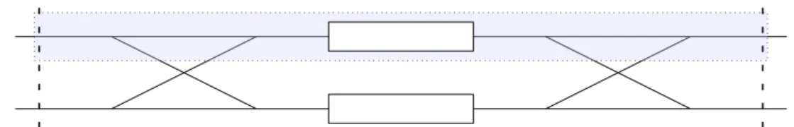
(a) Typical intermediate non-terminal station where one of the station areas is indicated by the colored rectangle. A train enters the station area if it enters the colored rectangle.
(b) Terminal station with two platforms, which can both be used for turning.
(c) A station with one extra platform, referred to as an intermediate terminal station. This platform is only connected with the tracks at one side and can be used for turning.
Figure 1: Three station types in a simple network. The vertical dashed lines situate the signals before and after the station. The white rectangles represent the platforms. The crosses at both sides of the platforms represent the switches and tracks that connect both platform areas.
in each intermediate terminal station, there is one extra platform for turning, (iv) the `assembling' of tracks coming from dierent terminal stations occurs within station areas. Everywhere outside the station areas there are bridges and tunnels to avoid the crossing of tracks. Moreover, overtaking is not allowed. For a visual representation of the dierent station types, see Figure 1.
A station area consists of the switches just before and after the station and the platform belonging to one direction to go through the station. So a station in a simple network consists of two station areas, one in each direction. This is illustrated in Figure 1a.
The occupation interval of a train in a station area is the time interval that the station area is occupied by that train and no other train can use the station area in this time interval. The occupation interval starts at the reservation time and ends at the release time. In this paper, the reservation time is a xed amount of time before the train enters the station area, independent of the station area. A train enters a station area when it passes the vertical dashed line in Figure 1a and enters the colored rectangle. The release
time in the model, and thus the occupation interval, is dened in such a way that it allows a next train to reserve the station area immediately after this release time. The release time thus guarantees that the train is already suciently far away when a next train wants to reserve the station area. As a result, the occupation interval will be somewhat longer than the time interval that a train will actually be in the station area in practice. The occupation interval of trains not dwelling in a station area, is articially lengthened such that the occupation time is equal to the occupation time of dwelling trains. This is to avoid undesired overtakings in the planning. The occupation time is the length of the occupation interval.
A conict occurs when (at least) two trains want to occupy the same station area at the same moment, so their occupation intervals for this station area overlap.
We dene the necessary turn time as the time for the train to enter the station area of the terminal station (decreasing speed), stopping at the platform, alighting and boarding of passengers, extra time needed by the driver to move from one side of the train to the other side and the time for the train to leave the station area of the terminal station again (increasing speed). The necessary turn time is in fact the shortest possible occupation time of a train in a terminal station.
The running time between two succeeding station areas is the time that a train needs between the release time of the rst station area and the reservation time of the next station area.
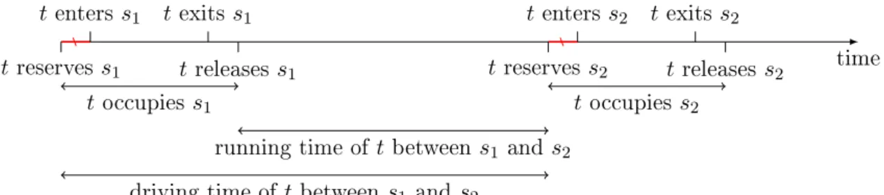
The drive time between two succeeding stations is dened as the occupation time of the rst station area and the running time to arrive at the next station area, so it is the time that a train needs between the reservation time of the rst station area and the reservation time of the next station area. Since the reservation time of a station area is dened as a xed amount of time before the entry time of that station, the drive time between two succeeding stations also coincides with the time between the entry times in these two stations. A visual representation is provided in Figure 2.
tenters s1 t exitss1 tenters s2 texits s2
t reservess1 treleasess1 treserves s2 t releasess2 time
toccupies s1 toccupies s2
driving time oft betweens1 ands2
running time oft between s1 ands2
Figure 2: Representation of the reservation time, the entry time, the release time, the exit time, the occupation time, the running time and the drive time of traintfor two succeeding
stationss1 ands2. The parts indicated in red are equally long, independent of the involved
train and stations.
These denitions can be made more general by not only looking at station areas, but at parts of the network bounded by signals.
We dene the buer time between two trains on a part of the network as the time between the time instant that the rst train releases that part of the network and the time instant that the other train reserves that same part of the network. The buer interval is the interval between these two time instants. It should be noted that, given the denition of occupation intervals in our paper, buer times of zero (or more) correspond to a normative macroscopically feasible timetable.
2.3 Timetabling
The goal of the timetabling module is to construct a passenger robust timetable. This avoids propagation of delays in case of small delays during daily operation in order to provide reliable travel times to the passengers and is achieved by maximizing the (minimum) buer times between train pairs. Parbo et al. (2016) give an extensive overview of passenger perspectives in railway timetabling. The PESP model of Serani and Ukovich (1989) is the foundation of many timetable models (e.g. Schrijver and Steenbeek, 1993; Nachtigall, 1996; Liebchen, 2006; Peeters, 2003; Schmidt and Schöbel, 2015; Groÿmann, 2011) and is also the framework of our timetabling model. The PESP model schedules events in a period of the cyclic timetable and takes precedence constraints and relations between events into account. Arrivals and departures of trains at stations or reservations and releases of track sections or station areas are events. If two events are related or can aect each other they form an activity. Examples of activities are the arrival and departure of the same train in a station or the reservation times of a shared switch, platform or station area by two dierent trains. The PESP model constrains each activity time, which is the time between the two events that dene the activity. The PESP is originally dened without an objective
function, but several objective functions for PESP can be found in the literature. We add an objective function that maximizes the (minimum) buer times between trains using the same part of the infrastructure, in order to achieve robustness. In our timetabling model, we also have `turning', `providing buer time' and `station' activities between events besides the usual running and transfer activities. Furthermore, we include extra constraints such that trains of the same line can be equally spread over the period of the cyclic timetable. These constraints coincide with the constraints for the synchronization activities considered in (Siebert and Goerigk, 2013). In that paper the impact of including line frequencies in cyclic timetabling is studied and the authors conclude that it positively and signicantly aects the quality of the constructed timetable. In Be²inovi¢ et al. (2016) and Goverde et al. (2016) an approach, dierent from PESP, is developed to obtain a stable robust and conict-free (and energy-ecient) timetable. This approach iterates between microscopic and macroscopic timetabling. Moreover, this approach includes a delay propagation model to compute delay recovery. However, this approach is more complex and works heuristically in comparison to the exact PESP approach and our approach. A recent and elaborate discussion on timetable literature in general and PESP in specic can be found in Sels et al. (2016).
2.4 Line planning
Railway line planning is, generally, the construction of a set of lines to operate in a rail network. There are parallels to line planning problems in bus network design and network design for liner shipping. Line planning for rail takes the physical rail network as a xed input, and provides a xed input to subsequent timetabling and rolling stock planning. So when creating the line plan, assumptions can potentially be made about the form or characteristics of timetables, rolling stock and rolling stock planning. Schöbel (2012) gives an overview of dierent approaches to model and solve the line planning problem, broadly categorizing line planning approaches that are (operator) cost-oriented, and those that are passenger-oriented.
Goossens et al. (2006) focus on minimizing operator cost, for the less-studied case of line planning where lines may not stop at every station. Also in our research the stopping pattern of a line is decided in the line planning problem. The advantage of allowing lines to skip stations is the potential to combine fast lines which only stop at the stations with high demand and slow lines which also stop at stations with low demand (with the classication of stations not specied but decided during line planning). Using fast lines shortens the travel time of a lot of passengers and the slow lines assure a service in every station.
With a passenger focus, a common objective function is to maximize the number of direct travelers, i.e. the number of passengers who have a route from their origin to des-tination that does not require transfers. The simplest interpretation of this objective is
to count the number of passengers for which there exists a line in the solution visiting both their origin and destination. This does not actually nd passenger routes and does not guarantee that all counted passengers can actually use the line, as there may be in-sucient capacity on some lines. Using this objective also has the risk in some networks that the passengers with no direct route may be faced with many transfers. Another dis-advantage is that maximizing the number of direct travelers encourages long train lines and, critically in our case, does not favour skipped stations. Bussieck et al. (1997) is one example which uses this direct traveler objective, while ensuring that direct lines also have sucient capacity to accommodate the passengers.
Another objective function with passenger focus is a travel time objective that takes into account the passenger's time traveling in trains and a penalty for switching trains (transfers). The calculation of this objective requires knowledge on the routing of pas-sengers in the network taking into account travel time and transfers. This routing of the passengers can be modelled as paths in a graph, potentially requiring one path for every pair of stations. Schöbel and Scholl (2006) and Borndörfer et al. (2007) are examples where passengers between a pair of stations are routed by minimizing the sum of the travel time costs of the used paths. This passenger routing objective could be used as part of a weighted sum objective along with some operator cost (Borndörfer et al., 2007), or used alone but with an additional operator cost budget constraint (Schöbel and Scholl, 2006). In some practical problems the inclusion of a budget can be very important when combined with a passenger-oriented objective, as without it, solutions can contain many lines to individually satisfy every type of passenger. Our line plan model uses also the passenger's travel time objective. In our case study, however, there are tight rate limits on the maximum num-ber of trains turning at a terminal station and on the use of certain infrastructure. Thus even without an operator budget consideration we do not risk solutions having particularly many lines.
Operator focused or passenger focused is a rst partitioning that can be made. Another partitioning is that a line planning model may be based on a predetermined set of lines (a line pool), or it may nd new lines dynamically. An advantage of a predetermined line pool is that all lines in the pool are guaranteed to be feasible in terms of line planning requirements, or advantageously for our case, in terms of timetabling requirements. This latter is explained in the next section. A predetermined pool also has the advantage of limiting the problem size in a useful and dynamic way (because the pool can be limited to be as diverse or as focused as desired). However, it has the disadvantage that the full set of possible lines may be large enough that enumerating them all would be intractable, while taking only a subset of all possible lines risks missing good solutions. Schöbel and Scholl (2006) present a model that takes as input a predetermined pool of lines. In contrast, Borndörfer et al. (2007) present a method where lines are generated dynamically in an
infrastructure network as a pricing problem, nding maximum-weighted paths to introduce as lines to a restricted master problem. However, the master problem itself is formulated in terms of a known line pool.
With respect to decision variables, many approaches are similar in using either a bi-nary decision for the presences of each line, or a non-negative or integral decision for the frequency of each line, where a frequency of zero means that the line is not in the solution. In our approach we may only select one of a set of frequencies dened individually for every line, so our model uses a binary decision variable indicating the presence of a (line, frequency)-pair.
Specically related to the problem we address at DSB S-tog, Rezanova (2015) solves the line planning problem with an operator focus, considering train driving time and a particular competing objective related to new regulations for drivers. The author notes the problem of nding line plan solutions that are not feasible for timetabling, and suggests that an integrated approach would be valuable.
Overall, our modelling approach is similar to the work of Schöbel and Scholl (2006) in the construction of the graph for passenger ows, but diers in the capturing of frequency-dependent costs for passenger travel times. We also model line frequency in a stricter manner which is necessary for our case study, where specic sets of frequencies are valid for each line where in contrast, other work such as Schöbel and Scholl (2006) or Borndörfer et al. (2007) models frequency as a discrete variable over all positive integers for each line.
3 Timetable-infeasibility
In this section we explain how limited shunt capacity and certain frequency combinations of lines that share a part of the network can lead to timetable-infeasibility of line plans. Our integrated approach uses these insights to construct line plans that allow normative macroscopically feasible and passenger robust timetables.
3.1 Line infeasibility
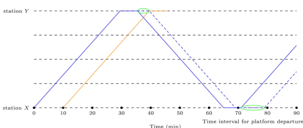
Consider Figure 3, showing a single train line operating at six times per hour between
terminal stationsXandY. The black dots on the time-axis show the scheduled departures
from station X for this line, which is once every ten minutes. We illustrate the rst two
time-distance graphs; the rst departing from station area X at minute zero (solid blue
line), and the subsequent train following at minute ten (red line). In this example, the travel
time between station areaXandY for the line is 29 minutes. This travel time includes the
running times between the stations and the occupation times of the intermediate stations (not in the terminal stations). We assume that the train has to turn on its platform in
0 10 20 30 40 50 60 70 80 90 stationX
stationY
Time interval for platform departure
Time interval for platform departure Time (min)
Figure 3: A line can be infeasible on its own
ten minutes later is therefore entering station areaY ten minutes later as well, so the rst
train has a well-dened latest departure of that station area which is marked as a dashed
blue line. The necessary turn time for this line in station Y is seven minutes. Note that
the necessary turn time already includes the occupation time of the terminal station Y
for the arriving train and the train driving back to station areaX, which share the same
rolling stock. So, this train is arriving in station areaX again between 65 minutes and 68
minutes after its rst departure at minute zero. The necessary turn time in station area
X is also seven minutes for this line. Thus, the train can leave station areaX for the next
round trip at 72 minutes after minute zero at the earliest (minute 65 arrival with seven minutes minimum necessary turn time) and 78 minutes at the latest (68 minute arrival with a maximum of ten minutes for dwelling and turning, assuming that the next train enters station areaX ten minutes later). However, no train is planned to leave station area
X in the interval of 72 to 78 minutes, which can be seen in Figure 3 as no black dot falls
in the interval indicated with the green line. Therefore no feasible timetable can be found for this line. We will call this line infeasibility.
This insight can be mathematically formulated as: If there exists no k∈Z+ such that
2Tl+ nttsl,0+ nttsl,|Sl| ≤ P fl k (1) and P fl k≤2Tl+ 2 P fl (2)
are satised, then, in case of restricted shunt capacity in its terminal stations, line l is
infeasible on its own. Here Sl ={sl,0,· · ·, sl,i, . . . , sl,|Sl|} is the set of all stations on line
l (independent on an actual stop), nttsl,0 and nttsl,|Sl| are respectively the necessary turn
time for line l in its start station sl,0 and end station sl,|Sl|, fl is the frequency of line l,
P is the period length of the cyclic timetable and Tl = Pie=0−1runl,sl,i,sl,i+1+ Pe−1
is the travel time of linel, whererunl,sl,i,sl,i+1 consists of the running time between station
sl,i andsl,i+1, andoccl,sl,i is the occupation time of stationsl,i. Furthermore, it is assumed
that trains of the same line are equally spread over the period and use the same platform in the terminal stations for passenger convenience.
So in the example above, Tl is 29 minutes, nttsl,0 and nttsl,|Sl| are seven minutes, P is
60 minutes and the line frequency fl is six.
Proof. We dene a train cycle of line l as (i) the trip from its start station to its end
station including running and dwelling, (ii) the turn movement in its end station, (iii) the trip from its end station to its begin station including running and dwelling and (iv) the turn movement in its begin station before the train can start a next cycle. The shortest
possible duration of a train cycle of linel is the sum of the running and occupation times
from the begin station to the end station, Tl, the necessary turn time in its end station,
nttsl,|Sl|, the travel time from the end station to the begin station,Tl(the travel time is the
same in both directions) and the necessary turn time in its begin station,nttsl,0. Note that the occupation times of the terminal stations,occsl,0 and occsl,|Sl|, are not included in Tl.
This shortest possible train cycle length is given in the left hand side (lhs) of formula (1). The longest possible duration diers from the shortest possible duration in the time that the train takes for turning in its terminal stations. Instead of only for the necessary turn time, the train may stay in the station area until the next train of the same line arrives, which isP/flminutes after its own arrival. ThisP/flminutes also includes the occupation
time of the arriving and departing train (same rolling stock). This maximal train cycle length is represented in the right hand side (rhs) of formula (2). Without loss of generality we can assume that train cycles of linelstart at{kP/fl|k∈Z+}. If linel is feasible, then for a train that starts its rst cycle atk0P/flfor ak0 ∈Z+, there has to exist ak∈Z+for the start of its next cycle such thatkP/fl ∈[k0P/fl+(lfs of (1)), k0P/fl+(rhs of (2))].
Remark that the latter statement remains true if k0P/fl is subtracted from both interval
bounds. This proves our mathematical insight by contraposition. As shown in the example,
such akdoes not always exist.
3.2 Frequency combination infeasibility
Suppose that two lines share a part of the network and that trains of the same line are equally spread in the cyclic timetable. A second insight is that the frequencies of these lines aect the minimum buer time between these lines. It is straightforward that the higher the frequencies the smaller the buer time between trains of these lines. But we also make the following claim:
Claim 1. The minimum buer time between a line at a higher frequency and a lower frequency is no greater than between two lines at the higher frequency.
Example Letfl≤fl0 be the frequencies of two lineslandl0 respectively. Iffl=fl0 = 5,
then on a given infrastructure resource, trains of lineland l0 could be planned alternately
every six minutes. Without loss of generality, we here assume occupation intervals of length zero, since any larger occupation interval will induce smaller buer times. However, if we assume fl = 4 and fl0 = 5. Then, at any infrastructure resource shared by line l and l0
and exactly once in the period of the timetable, there will be two succeeding trains of line
l0 which are planned between two succeeding trains of l (pigeon hole principle). We will
refer to the trains of linel and l0 that are concerned in this event as t1l,r, tl,r2 , t1l0,r and t2l0,r
respectively, wherel and l0 are the lines concerned,r represents the shared infrastructure
resource and the superscript indicates the order of the trains:t1
l,r (t1l0,r) proceeds traint2l,r
(t2l0,r). In this example, the time betweent1l,r andt2l,r to equally spread the trains of linelis
15 minutes and 12 minutes betweent1l0,randt2l0,r for linel0. This would lead to the situation
in Figure 4, whereais the buer time betweent1l,r andt1l0,r atr. In order to tt1l0,r andt2l0,r
between t1l,r and t2l,r, ahas to be strictly smaller than three. So, the smallest buer time
between a train of lineland linel0 at r is smaller than or equal to one-and-a-half minutes,
which is much smaller than the six minutes in casefl=fl0 = 5. The shared infrastructure
resource, that is mostly referred to in this paper, is a station area.
t1l,r t1
l0,r t2l0,r t2l,r
0 0a0 a+ 12 15 time (min)
Figure 4: If linesl and l0 have frequenciesfl = 4and fl0 = 5 respectively, then once in 60
minutes two trains (t1l0,r and t2l0,r) of line l0 will pass in between two trains (t1l,r and t2l,r) of
line l at shared infrastructure resource r. Without loss of generality we can assume that
this happens in the rst quarter. Herea∈Rand 0< a <3.
The minimum buer time between two lines at a shared infrastructure resource can be
bound by the following formula: The minimum buer time between line l and line l0 with
frequencies fl≤fl0 respectively, on a shared infrastructure resource, is smaller than (≤) P fl −(d fl0 fle −1) P fl0 2 (3)
where P is the period length of the cyclic timetable, dxe equals the smallest integer y with
y≥x and trains that operate on a line are equally spread over the period.
Proof. Letr be a shared infrastructure resource of linelandl0. Without loss of generality,
we here assume occupation intervals of length zero, since any larger occupation interval will induce smaller buer times. By the pigeon hole principle, there are two trains of line
lin between which dfl0/fletrains of line l0 are passing atr. With the same notation as in
the example above, we chronologically havet1l,r, t1l0,r,· · ·, t dfl0/fle
are spread byP/fl minutes and traint1l0,r and t dfl0/fle
l0,r by (dfl0/fle −1)P/fl0 minutes. So,
the buer time betweent1l,r and t1l0,r plus the buer time betweent dfl0/fle
l,r and t2l0,r equals
P/fl−(dfl0/fle −1)P/fl0. Thus at least one of these two buer times is smaller than half
of this value, which is the bound given in (3).
If the upper bound in (3) is strictly smaller than the minimum necessary buer time according to safety regulations in the network, thenlwith frequencyflandl0with frequency
fl0are not feasible together. In the example, if the minimum necessary buer time according
to safety regulations is two minutes, then these lines l and l0 cannot be combined at
frequenciesfl= 4 and fl0 = 5.
Proof of Claim 1. We rst show that expression (3) is bounded above byP/2fl0. We can
write
fl0 =αfl+β, (4)
withα, β∈Z+ andβ < fl. Then we have: P fl −(d fl0 fle −1) P fl0 2 = P 2fl0 f l0−(dfl0 fle −1)fl fl , = P 2fl0 αf l+β−(dαffl+β l e −1)fl fl = P 2fl0 αf l+β−(α+dfβle −1)fl fl = P 2fl0 β− dβ flefl+fl fl ≤ P 2fl0. (5)
Formula (3) is maximal in case fl0 equals or is a multiple offl (fl0 =kfl,k∈Z+): P fl−(d kfl fle −1) P kfl 2 = P fl −(k−1) P kfl 2 = kP−(k−1)P 2kfl = P 2kfl = P 2fl0. (6)
4 Methodology
In this section, we propose an integrated approach that constructs a line plan from scratch that minimizes a weighted sum of operator and passenger cost and allows a feasible and robust timetable. First a timetable-feasible line plan is constructed. Then, iteratively and interactively, a line planning module produces a line plan, and for that line plan, a timetable module produces a timetable that maximizes the (minimum) buer times between train pairs. In each iteration an analysis of the timetable indicates how the line plan could be
adapted in order to allow a more robust timetable. This adaptation increases the exibility of the line plan which is used, in the timetabling module, to increase the minimum buer times. The line plan module then calculates a new line plan that includes this adaptation while minimizing the weighted sum of operator and passenger costs. This feedback loop stops when there is no further improvement possible or if there is no improvement during a xed number of iterations for the minimum buer times between train pairs.
We rst discuss the line planning module and the timetabling module separately and then the integration of both. Both the timetable and the line planning module consist of an exact optimization model, though our combined approach, and the fact that we do not always solve the models to optimality, result in an overall heuristic method.
4.1 Line planning module
Constructing a line plan consists of selecting a set of lines which meet certain requirements from a pool of predetermined lines. The line pool is not exhaustive; there are many more possible lines than those considered, but the set is reduced to those that meet certain cri-teria as discussed with the rail operator. This also keeps the problem size small. The model performs three functions: (i) selecting the lines and frequencies and creating a valid plan, (ii) routing passengers between origin and destination stations and (iii) relating passenger routes to line selections.
Let us rst dene the set of all lines available:L. For every linel∈Lwe dene a set of valid frequencies for the line:Fl. The operator must meet certain obligations for any valid
line plan and must not exceed certain operational limits. These restrictions are referred to
as service constraints. We dene these all in terms of a set of resourcesR, and dene all
limitations as either a minimum (rminr) or maximum (rmaxr) number of trains using that
resourcer ∈R every hour. The subset of lines that make use of resourcer ∈R is dened
asLr. Letcl,f be the cost to the operator for operating line lat frequency f.
The line planning module starts from a known origin-destination (OD) matrix contain-ing the passenger demand for travel between every origin and destination, where origins
and destinations are simply stations in the rail network. Let S be the set of stations. For
two stations s1, s2 ∈ S we know the demand ds1,s2. We model passengers as a ow from
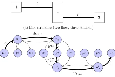
each origin station to every relevant destination station in a graph. The structure of this graph (nodes and edges) is uniquely determined (i) by the network (stations and station links) and (ii) by the lines considered in the line pool. Furthermore, this graph captures the passenger cost in terms of drive time on lines and estimated transfer time between lines in case a transfer is required (estimated based on the frequency). We refer to this graph as the passenger graph. We now explain the construction of this passenger graph in more detail. An example can be found in Figure 5 for a network with three stations, 1, 2 and 3, and two lineslandl0 visiting two of the stations each. A passenger graph contains a (line,
1
2
3
l
l0
(a) Line structure (two lines, three stations)
p2 n2 µ2 σ2 n1 n02 n03 Kx Kfvar l0 p1 µ1 σ1 µ3 p3 σ3 0 0 drl,1,2 drl0,2,3
(b) Corresponding passenger graph structure
Figure 5: The upper gure shows a simple network with three stations 1, 2 and 3, and two lines l and l0. Line l visits stations 1 and 2, and line l0 visits stations 2 and 3. Each line
operates at just a single frequency (fl, fl0 ∈ Z+). The lower gure shows the subsequent
passenger graph structure used for this network. We simplied the notation to keep the gure clear: node n1 and n2 represents node (l, fl,1) and (l, fl,2) respectively and node
n02 and n03 represents (l0, fl0,2)and (l0, fl0,3)respectively. Costs are labelled on the edges
for a passenger travelling from station 1 to station 3, transferring lines at station 2, with used edges in bold. The costs to the passenger aredrl,1,2, travelling (driving) on linelfrom
station 1 to 2; xed cost Kx for a transfer and an additional Kfvar
l0 frequency dependent
cost for transferring to linel0; and drl0,2,3 travelling on line l0 from station 2 to 3.
frequency, station) vertex for every line, frequency, and every station visited by that line. The edges of this graph represent travel possibilities, with the edge cost being the known train driving time or the estimated transfer time. Additionally, for every stationswe have
a platform vertex ps with edges from and to every (line, frequency, s) vertex, where the
costs correspond to an estimate of perceived transfer time which consists of a xed penalty
component and a frequency-dependent component. Finally, this graph contains sourceµs
and sinkσs vertices for every stationswhere passengers originate from or terminate their
travel. These vertices are connected to the appropriate (line, frequency, station) vertices with edges representing boarding or alighting from a line. These edges have zero cost. We model source and sink vertices separately to ensure line-to-line transfers are only possible via the platform vertex incurring the frequency-dependent costs.
Let V and E be the set of all vertices and edges of this graph, respectively, andτe be
• Type 1. From(l, f, s)to(l, f, s0)for all linesl∈L,f ∈Flandsands0two succeeding
stations visited by linel.
• Type 2. From(l, f, s) to ps for all lines l∈L,f ∈Fl and sa station visited by line
land ps the platform vertex of station s.
• Type 3. Fromps to (l, f, s) for all lines l∈L,f ∈Fl and sa station visited by line
land ps the platform vertex of station s.
• Type 4. From µs to(l, f, s) for all lines l∈L,f ∈Fl ands a station visited by line
land µs the source vertex of stations.
• Type 5. From(l, f, s) to σs for all linesl∈L,f ∈Fl andsa station visited by line
land σs the sink vertex of stations.
This graph is similar to the change&go graph of Schöbel and Scholl (2006), but distin-guishes between line transfers that in our case happen to lines with discrete frequencies, with a frequency-dependent cost. A more complex example with multiple frequencies per line can be found in Appendix A.
Let le be the line that edge e is related to and fe be the frequency of the line that e
is related to. This line and frequency of an edge are uniquely dened as the two vertices
connected by edgeeare either both related to the same line and frequency or only one of
them is related to a line and frequency.
Let asv be the ow of passengers originating from station s that enters vertexv minus
the ow of passengers originating from station s leaving vertex v, where v is a vertex of
the passenger graph. For verticesv of type (line, frequency, station) or platform vertices, asv = 0 for all stations s∈S. All passengers that enter such a vertex, also leave again. For vertices v which are source vertices for a certain station s, passengers are only leaving to
other stations according to the demand: asv =−P
s0∈Sds,s0. For vertices v which are sink
vertices for a certain stations, passengers coming from other stations s0 are only entering: asv0 =ds0,s for all stationss0 ∈S.
For relating passengers to lines, letCf be the passenger capacity of any line operating
at frequencyf. We are therefore assuming the same rolling stock unit type and sequence for
every line, but a higher frequency provides more seats than a lower frequency. We require that no more passengers use a line as the line capacity permits for the frequency the line is operating at.
We use two classes of decision variables: xl,f ∈ {0,1} is a binary decision variable
indicating whether or not line l is selected at frequency f, and ye
s decides the number of
passengers from origin stations that use edgeein the passenger graph.
The line planning model is:
Minimize λX l∈L X f∈Fl cl,fxl,f+ (1−λ) X e∈E X s∈S τeyse (7)
s.t. X f∈Fl xl,f ≤1 ∀l∈L (8) X l∈Lr X f∈Fl f xl,f ≥rminr ∀r∈R (9) X l∈Lr X f∈Fl f xl,f ≤rmaxr ∀r∈R (10) X (u,v)∈E ys(u,v)− X (v,w)∈E ys(v,w) =asv ∀s∈S,∀v∈V (11) X s∈S yes ≤Cfxle,fe ∀e∈E (12) xl,f ∈ {0,1} ∀l∈L, f ∈Fl (13) yes∈R+ ∀s∈S, e∈E (14)
The objective function (7) is a weighted sum of the operator cost and the passenger
travel time (drive time and transfer time), using a parameter λ∈ [0,1] to determine the
importance of one component over the other.
Constraints (8) ensure that a line is chosen with at most one frequency (i.e. combina-tions of frequencies are not permitted, as if valid a discrete frequency would be present in the frequency set Fl for the line). Constraints (9) and (10) ensure that the obligatory and
operational requirements are met for the line plan. Constraints (11) consist of the ow con-servation constraints. The number of passengers leaving from an origin station must ow from that station with the appropriate number arriving at every destination station, such that ow is conserved. Constraints (12) link the ows of passengers to the line decisions. The presence of a positive passenger ow on an edge in the graph is dependent on some line being present in the plan. The maximum ow on that edge depends on the passenger capacity of the corresponding line at the appropriate frequency. Finally, constraints (13) and (14) restrict the line variables and ow variables to be binary variables and positive otherwise unrestricted variables, respectively.
The model requires|E||S|ow decision variables, which is large due to the many edges
in the described passenger graph. However, we observe that many of the vertices and edges in the graph are very similar and dier only in line frequency. For lines with many possible frequencies there is signicant duplication. For the edges related to a transfer at a station, the frequency is required to determine the cost to the passenger. However for all other edges the frequency information is redundant. Indeed, the cost of travelling on a line between stations does not depend on the frequency of that line. A rst simplication of the model is that for each line and its frequencies, we replace the edges (and vertices) which do not depend on frequency with an edge (and vertex) related only to line and station instead of line, frequency and station. This is shown in Figure 6. The capacity of the replacement
edge (and resulting right hand side of constraints (12)), is given by P f∈FlCfxl,f. p mα mβ mγ µ σ
(a) Original graph structure
p mα,β,γ
µ σ
(b) Reduced graph structure
Figure 6: The full and reduced graph structure for a single linel with three frequencies,α,
β and γ inZ+, at a single station s. We simplied the notation to keep the gure clear:
nodemi represents node(l, i, s)for frequencyi∈ {α, β, γ}. Nodemα,β,γ is the replacement
node of nodesmα, mβ and mγ in the reduced graph structure.
Figure 6 shows the graph structure for a single station and a single line with three fre-quencies as originally described (Figure 6a) and with the explained reductions (Figure 6b).
Nodes µ and σ are respectively the station source and sink vertices for passengers andp
is the platform vertex for that station. The verticesmα,mβ,mγ are the (line, frequency,
station) vertices for the three considered frequencies of the line, in that station. The red edges are the transfer edges (though no other lines are shown). Edges connecting these verticesmα,mβ, and mγ to corresponding vertices at other stations are not shown. Vertex
mα,β,γ is the combination of the verticesmα,mβ, andmγ. The edge betweenµandmα,β,γ,
and betweenmα,β,γ andσ, is the combination of the edges betweenµandmα,mβ, andmγ
in (Figure 6a), andmα,mβ, and mγ andσ, respectively. In Appendix A a more complex
example of a passenger graph reduction can be found.
A second simplication of the model is that we consider transfer edges only at a minimal set of transfer stations. This set of stations is xed beforehand and suces to facilitate all optimal passenger ows, when every passenger's origin-destination pair is considered individually. Any solution that is feasible for this restricted problem is feasible if transfers edges are included for any station, but some solutions that are feasible if transfers are permitted anywhere may not be feasible with the restriction (although we have not observed this). At stations where we do not permit transfers we do not include transfer edges, and this reduces the total number of edges in the graph by between 23% and 34% when tested for a range of line pools. Finally, we can determine that only a subset of all edges should be used for the ows from a given origin station; generally it is never true that in an optimal solution passengers will be assigned an edge that travels towards the station
they originate from. This is a third measure to simplify the model.
By making these three alterations we nd that the line planning problem is solvable directly as a MILP, though not to optimality in the time frame we require. For our tests, nding line plans with no other restriction, we use a time limit of one hour, or until a
gap between the solution and best lower bound is below0.5%(in most cases the gap limit
is reached, but for some weightings of objectives, one hour is insucient). However, for a reduced line pool that we use in the integrated approach described later, the problem becomes easier and is solvable to optimality in an acceptable time frame.
The formulation (7)(14) denes the basic line planning model. However, when search-ing for line plans that only dier a little from a given line plan we may impose some additional restrictions. The simplest types are the following:
X l∈L X f∈Fl f xl,f ≥k1 (15) X l∈L X f∈Fl f xl,f ≤k2 (16)
That is, we require that the total number of (one-directional) trains running in the network per hour is between some upper and lower bound. This may be, for example, to nd solutions that do not dier too much from some original solution. We use this because, from the point of view of the timetable module, two solutions that dier only in line frequency but not in line routes can be very dierent. Without such constraints, when seeking a line plan that is similar but dierent to a given plan, a change of frequency would not maintain the similarities in timetabling that we seek. Now, suppose we are given a line plan or a partial line plan, in the form X ={(l, f),(l0, f0),(l00, f00), ...} where every
(l, f) in X is a valid line and frequency combination, and that this (partial) line plan
should not be in the solution. Then we may impose the following constraint for every such line plan:
X
(l,f)∈X
xl,f ≤ |X| −1. (17)
Such constraints are used to forbid solutions we have already discovered and do not wish to nd again, and also to forbid partial solutions which we already know are problematic for timetabling, i.e. they lead to timetable-infeasibility. Finally, and similarly, we may have some given line planX and desire that the solution line plan contains at leastklines from
the plan:
X
(l,f)∈X
xl,f ≥k. (18)
Such constraints ensure that a discovered line plan is similar to some previous line plan, while diering by some number of (unspecied) lines. If instead the lines that may dier
are specied, we can x the variables of the lines that may not dier and only permit those variables corresponding to the specied lines that may dier to change (along with variables corresponding to lines not in the plan). These extra restrictions are used in the integrated approach when looking for a similar line plan that is more exible, i.e. allows a more robust timetable.
4.2 Timetabling module
The timetable module is based on a PESP model. We indicate our event-activity network as (E,A). The set of trains is indicated as T, the set of lines in the line plan (output of
the line planning module) as X, the line operated by traint is indicated as `t, the set of
station areas is S and the set of station areas on a line l (independent of an actual stop
in these stations) is indicated as Sl. As we assume a railway network with limited shunt
capacity, our model assumes that all the trains can and must turn on their platform at end stations. The setTturn contains the train couples(t, t0) for which it holds that t becomes
train t0 after turning on the platform in its end station. Trains t and t0 share the same
rolling stock. Line `t and `t0 contain the same stations but in opposite direction. The set
Tline spread contains the train couples(t, t0) wheretand t0 are two succeeding trains of the
same line, i.e. no other train operating on the same line drives in between them.
The event set Eof the event-activity network consists of the following events.
• The reservation of a station area s by a train tis a reservation event (t, s,res). We
deneEresas{(t, s,res)| ∀t∈T, s∈S
`t}.
• The release of a station areasby a traintis a release event (t, s,rel). We deneErel
as{(t, s,rel)| ∀t∈T, s∈S`t}.
• The reservation of a platformρs˜t,tby a traintin its terminal station˜stin order to turn
is a platform reservation event(t, ρs˜t,t,res). We deneE
res,pas{(t, ρ
˜
st,t,res)| ∀t∈T}. • The release of a platformρ˜st,t by a train tin its terminal stations˜tin order to turn
is a platform release event (t, ρ˜st,t,rel). We deneE
rel,p as{(t, ρ
˜
st,t,rel)| ∀t∈T}.
The following inclusions holdEres,p⊂Eres⊂EandErel,p⊂Erel ⊂EandE=Eres∪Erel. So
platformρs˜t,t of traintin its terminal station can be interpreted as an extra station where
the train arrives after arriving in its terminal station ˜st. Note that the event set consists
here of station reservation and release times instead of the more common arrival and departure times in stations. From a macroscopic viewpoint these reservation and release times of a station area can be used to derive arrival and departure times on the platforms. Since we did not construct the timetable on the signaling level, we cannot fully guarantee that a timetable that is feasible according to our model is conict-free in practice on the
microscopic level. However, all the timetables constructed during our case study that were checked by the railway operator, were found to be suitable to implement in practice.
The activity setAcontains:
• running activities between the release of a train in a station and the reservation
of this train of the next station on its line. Let Arun = {((t, s,rel),(t, s0,res)) ∈
Erel×Eres| ∀t∈T and sands0 succeeding stations of ` t};
• station activities between the reservation and the release of a train in a station on
its line. LetAstation ={((t, s,res),(t, s,rel))∈Eres×Erel| ∀t∈T, s∈S
`t\ {ρs˜t,t}}; • turn activities between the reservation and the release of a train on its platform in its
terminal station. LetAturn ={((t, ρ ˜
st,t,res),(t, ρs˜t,t,rel))∈E
res,p×Erel,p| ∀t∈T};
• buer activities between the release of one train and the reservation of another train
in the same station area. Let Abuffer = {((t, s,rel),(t0, s,res)) ∈ Erel ×Eres| ∀t, t0 ∈
T :t6=t0, s∈S`t ∩S`0t};
• line spread activities between the reservations of two succeeding trains on the same
line in the stations on their line. Let Aline spread = {((t, s,res),(t0, s,res)) ∈ Eres× Eres| ∀t, t0 ∈T : (t, t0)∈T
line spread, s∈S`t};
• turn connection activities between the release of a train of the platform in its end
station and the release of the next train of the opposite line that leaves from that station area. Let Aturn-con = {((t, ρ
˜
st,t,rel),(t
0,s˜
t,rel)) ∈ Erel,p ×Erel| ∀t, t0 ∈ T :
(t, t0)∈Tturn}. This next train is the same physical train.
As mentioned in Section 2, we want to maximize the minimum buer times between train pairs. In terms of the event-activity graph, we want to maximize the minimum activity time of the buer activities. Mathematically we have
max min
a=(i,j)∈Abuffer(πj −πi+kaP), (19)
where πi and πj are the event times of event i and j respectively which dene together
a buer activity. However, this objective function is not linear, but as it is a max-min objective function, it can easily be linearized. Therefore, we introduce an auxiliary variable
z∈[0, P], whereP is the period length of the cyclic timetable. We add the constraints z≤πj−πi+kaP ∀a= (i, j)∈Abuffer (20)
and we change the objective function to the maximization ofz:maxz. The complete model
is then the following.
z≤πj −πi+kaP ∀a= (i, j)∈Abuffer
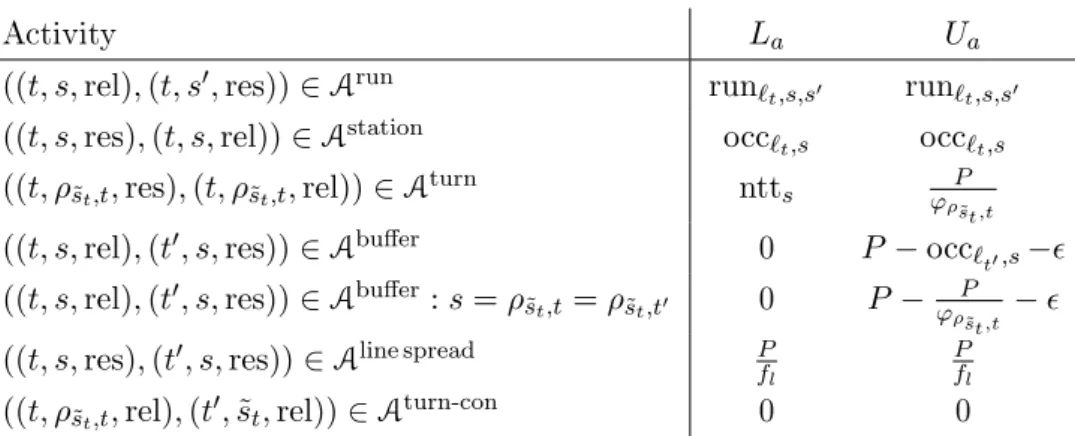
La≤πj−πi+kaP ≤Ua ∀a= (i, j)∈A (22)
0≤πi< P ∀i∈E (23)
ka∈ {0,1} ∀a= (i, j)∈A (24)
Constraints (22) bound all activity times from below and above. The term kaP avoids
negative activity times. To ensure a unique value forka, the value ofUa has to be smaller
than the period length P. The specic values of Ua and La are listed in Table 1 for all
activitiesa∈A. The running activity times are bounded by the time that a train of linel
needs between the release of a stationsand the reservation of the next stations0, indicated
asrunl,s,s0. The running time between the terminal station of a train and the platform in
its terminal station is zero minutes. The station activity times are bounded by the time that is necessary and provided for a linelto occupy a stations, indicated asoccl,s. This is
the time between the reservation and release time of that station. The turn activity times
are bounded by the necessary turn time in the terminal station s, which is indicated as
nttsand the time from which on a next train can arrive on that platform. Trains that make
use of the same turn platform all get the same maximum time to stay on that platform which is equal to the period length of the cyclic timetable divided by the number of trains that turn on platformp. The number of trains that turn on platformp is indicated asϕp.
The buer activity times have to be positive and smaller thanP−occ`t,s−to ensure that
occupation intervals do not overlap, independently of the order of both trains that will be assigned. On platforms in terminal stations the upper bound is smaller because trains
occupy the platform for a longer time, i.e. the upper bound in our model isP−ϕP
ρ˜st,t −.
Before initializing the timetable module, a check is necessary to determine if too many
trains are scheduled on one platform, i.e. P
ϕp ≥nttsmust be satised. If so, the trains have
enough time for turning, otherwise the timetable will be infeasible. The value ofdepends
on the time discretization. We use 0.1 minutes. In this model we equally distribute trains of a line over the period, and therefore the line spread activity times have to be equal to
the period length divided by the line frequency. The frequency of a line l is indicated as
fl. The turn connection activity times have to be equal to zero, ensuring that the `turning'
platform is freed if the next train leaves in the opposite direction.
4.3 Integrated approach
Here, we explain how the line planning and timetabling module can be integrated to construct a line plan and timetable that induce a low passenger and operator cost and maximize the buer times between train pairs in order to provide a passenger robust railway schedule. The line planning and timetabling module work iteratively and interactively. The line planning module creates an initial line plan which is evaluated by the timetabling
Activity La Ua
((t, s,rel),(t, s0,res))∈Arun run
`t,s,s0 run`t,s,s0 ((t, s,res),(t, s,rel))∈Astation occ
`t,s occ`t,s ((t, ρs˜t,t,res),(t, ρ˜st,t,rel))∈A turn ntt s ϕρP ˜ st,t ((t, s,rel),(t0, s,res))∈Abuffer 0 P−occ
`t0,s−
((t, s,rel),(t0, s,res))∈Abuffer:s=ρ ˜
st,t=ρs˜t,t0 0 P−
P ϕρst,t˜ − ((t, s,res),(t0, s,res))∈Aline spread P
fl P fl ((t, ρs˜t,t,rel),(t 0,˜s t,rel))∈Aturn-con 0 0
Table 1: Lower and upper bounds for the PESP constraints (22)
module. Based on the minimum buer times between line pairs, a critical line in the line plan is identied. The line planning module then creates a new line plan with at least one dierent line, i.e. the time length of this critical line is changed. The goal is to create more exibility in the line plan. This exibility will be used by the timetabling module to improve its robustness. This heuristic approach which is divided into two parts is now further explained. In Figure 7, a visual overview of the algorithm is presented and in Section 6.2 we apply the approach to an example.
Line plan Model Minimizing operator cost Minimizing passenger cost
Timetable Model Maximizing (selection of)
minimal buer times Timetable-feasible line plan
Critical line(s) Modied line plan(s)
Stop if minimal buer times do not improve
Figure 7: Overview of the integrated approach Part 1: Initialization
Step 1: Construct an initial line plan
We construct a line plan that satises service constraints and optimizes a weighted sum of the passenger and operator cost with the line planning mod-ule. Beforehand, we check for infeasible lines in the line pool as discussed in Section 3. We check with the timetable module if a feasible timetable can be