Cache Oblivious Search Trees via Binary Trees of Small Height
Gerth Stølting Brodal
∗Rolf Fagerberg
∗Riko Jacob
∗Abstract
We propose a version of cache oblivious search trees which is simpler than the previous proposal of Bender, Demaine and Farach-Colton and has the same complex-ity bounds. In particular, our data structure avoids the
use of weight balancedB-trees, and can be implemented
as just a single array of data elements, without the use of pointers. The structure also improves space utilization. For storingn elements, our proposal uses (1 +ε)n
times the element size of memory, and performs searches
in worst case O(logBn) memory transfers, updates
in amortized O((log2n)/(εB)) memory transfers, and
range queries in worst case O(logBn+k/B) memory
transfers, wherekis the size of the output.
The basic idea of our data structure is to maintain a dynamic binary tree of height logn+O(1) using existing methods, embed this tree in a static binary tree, which in turn is embedded in an array in a cache oblivious fashion, using the van Emde Boas layout of Prokop.
We also investigate the practicality of cache oblivi-ousness in the area of search trees, by providing an em-pirical comparison of different methods for laying out a search tree in memory.
1 Introduction
Modern computers contain a hierarchy of memory lev-els, with each level acting as a cache for the next. Typi-cal components of the memory hierarchy are: registers, level 1 cache, level 2 cache, main memory, and disk. The time for accessing a level in the memory hierarchy increases from one cycle for registers and level 1 cache to figures around 10, 100, and 100,000 cycles for level 2 cache, main memory, and disk, respectively [13, p. 471], making the cost of a memory access depend highly on what is the current lowest memory level containing the element accessed. The evolution in CPU speed and memory access time indicates that these differences are
∗BRICS (Basic Research in Computer Science, www.brics.dk,
funded by the Danish National Research Foundation), De-partment of Computer Science, University of Aarhus, Ny Munkegade, DK-8000 ˚Arhus C, Denmark. E-mail:
{gerth,rolf,rjacob}@brics.dk. Partially supported by the FET part of the IST Programme of the EU under contract number IST-1999-14186 (ALCOM-FT).
likely to increase in the future [13, pp. 7 and 429]. As a consequence, the memory access pattern of an algorithm has become a key component in determining its running time in practice. Since classic asymptotical analysis of algorithms in the RAM model is unable to capture this, a number of more elaborate models for analysis have been proposed. The most widely used of these is the I/O model of Aggarwal and Vitter [1], which assumes a memory hierarchy containing two levels, the
lower level having sizeM and the transfer between the
two levels taking place in blocks of B elements. The
cost of the computation in the I/O model is the number of blocks transferred. This model is adequate when the memory transfer between two levels of the memory hierarchy dominates the running time, which is often the case when the size of the data significantly exceeds the size of main memory, as the access time is very large for disks compared to the remaining levels of the memory hierarchy.
Recently, the concept ofcache oblivious algorithms
has been introduced by Frigo et al. [12]. In essence, this designates algorithms optimized in the I/O model,
except that one optimizes to a block size B and a
memory size M which are unknown. This seemingly
simple change has significant consequences: since the analysis holds for any block and memory size, it holds
for all levels of the memory hierarchy. In other words,
by optimizing an algorithm to one unknown level of the memory hierarchy, it is optimized to each level automatically. Furthermore, the characteristics of the memory hierarchy do not need to be known, and do not need to be hardwired into the algorithm for the
analysis to hold. This increases the portability of
implementations of the algorithm, which is important in many situations, including production of software libraries and code delivered over the web. For further details on the concept of cache obliviousness, see [12].
Frigo et al. [12] present optimal cache oblivious al-gorithms for matrix transposition, FFT, and sorting. Bender et al. [5], give a proposal for cache oblivious search trees with search cost matching that of standard
(cache aware) B-trees [4]. While most of the results
in [5, 12] are of theoretical nature, [12] contains some preliminary empirical investigations indicating the com-petitiveness of cache oblivious algorithms. The authors
declare the determination of the range of practicality of cache oblivious algorithms an important avenue for future research.
In this paper, we study further the subject of cache oblivious search trees. In the first part, we propose a simplified version of the cache oblivious search trees from [5], achieving the same complexity bounds. In particular, our data structure avoids the use of weight
balanced B-trees of Arge and Vitter [3], and it can be
implemented in a single array of data elements without the use of pointers. Our structure also improves space utilization, implying that for givenn, a larger fraction of the structure can reside in lower levels of the mem-ory hierarchy. The lack of pointers also makes more elements fit in a block, thereby increasing the
parame-ter B. These effects tend to decrease running time in
practice. For storingnelements, our data structure uses (1 +ε)ntimes the element size of memory. Searches are
performed in worst case O(logBn) memory transfers,
updates in amortized O((log2n)/(εB)) memory
trans-fers, and range queries in worst case O(logBn+k/B)
memory transfers, where k is the size of the output.
This matches the asymptotic complexities of [5]. We note that as in [5], the amortized complexity of updates can be lowered by the technique of substituting leaves
with pointers to buckets each containing Θ(logn)
ele-ments and maintaining the size bound of the buckets by splitting (merging) overflowing (underflowing) buckets. The price to pay is that ranges cannot be reported in
the optimal number Θ(k/B) of memory transfers, since
the buckets can reside in arbitrary positions in memory. The basic idea of our data structure is to maintain
a dynamic binary tree of height logn +O(1) using
existing methods [2, 14], embed this tree in a static binary tree, which in turn is embedded in an array in a cache oblivious fashion, using the van Emde Boas layout [5, 19, 22]. The static structures are maintained by global rebuilding, i.e. they are rebuilt each time the dynamic tree has doubled or halved in size.
In the last part of this paper, we try to assess more systematically the impact of the memory layout of search trees by comparing experimentally the effi-ciency of the cache-oblivious van Emde Boas layout with a cache-aware layout based on multiway trees, and with classical layouts such as Breath First Search (BFS), Depth First Search (DFS), and inorder. Our results indicate that the nice theoretical properties of cache oblivious search trees actually do carry over into prac-tice. We also implement our proposal, and confirm its practicality.
1.1 Related work. One technique used by our data structure is a cache oblivious layout of static binary
search trees permitting searches in the asymptotically optimal number of memory transfers. This layout, the
van Emde Boas layout, was proposed by Prokop [19, Section 10.2], and is related to a data structure of van Emde Boas [21, 22].
Another technique used is the maintenance of bi-nary search trees of height logn+O(1) using local re-buildings of subtrees. The small height of the tree allows it to be embedded in a perfect binary tree (a tree with 2k
−1 internal nodes and optimal height) which has only
a constant factor more nodes. Techniques for maintain-ing small height in binary trees were proposed by Ander-sson and Lai [2], who gave an algorithm for maintaining height⌈log(n+ 1)⌉+ 1 using amortizedO(log2n) work per update. By viewing the tree as a linear list, this problem can be seen to be equivalent to the problem of
maintaining n elements in sorted order in an array of
length O(n), using even redistribution of the elements in a section of the array as the reorganization primitive during insertions and deletions of elements. In this for-mulation, a similar solution had previously been given by Itai et al. [14], also using amortized O(log2n) work
per update. In [9], a matching Ω(log2n) lower bound
for algorithms using this primitive was given.
Both the van Emde Boas layout and the technique of Itai et al. were used in the previous proposal for cache oblivious search trees [5]. The difficulty of this proposal originates mainly from the need to change the van Emde Boas layout during updates, which in turn necessitates the use of the weight balancedB-trees of Arge and Vitter [3]. By managing to use a static van Emde Boas layout (except for occasional global rebuildings of the entire structure), we avoid the use of weight balancedB-trees, and arrive at a significantly simpler structure.
Another improvement in our data structure is to avoid the use of pointers. The termimplicitis often used for pointer-free implementations of trees and other data structures which are normally pointer based. One early example is the heap of Williams [23]. There is a large body of work dealing with implicit data structures, see e.g. [7, 11, 18] and the references therein. In that work, the termimplicit is often defined as using only space for
the n elements stored, plusO(1) additional space. In
the present paper, we will abuse the terminology a little, takingimplicit to mean a structure stored entirely in an array of elements of lengthO(n).
We note that independently, a data structure very similar to ours has been proposed by Bender et al. [6]. Essentially, their proposal is leaf-oriented, where ours is node-oriented. The leaf-oriented version allows an easy implementation of optimal scanning from any given lo-cation (the node-oriented version needs successor
point-ers for this), whereas the node-oriented vpoint-ersion allows an implicit implementation, with the associated increase
in B and decrease in memory usage.
The impact of different memory layouts for data structures has been studied before in different contexts. In connection with matrices, significant speedups can be achieved by using layouts optimized for the memory hierarchy—see e.g. the paper by Chatterjee et al. [8] and the references it contains. LaMarca and Ladner consider
the question in connection with heaps [16]. Among
other things, they repeat an experiment performed by Jones [15] ten years earlier, and demonstrate that due to the increased gaps in access time between levels in
the memory hierarchy, the d-ary heap has increased
competitiveness relative to the pointer-based priority
queues. For search trees,B-trees are the standard way
to implement trees optimized for the memory hierarchy. In the I/O-model, they use the worst case optimal number of memory transfers for searches. For external memory, they are the structure of choice, and are widely used for storing data base indexes. Also at the cache level, their memory optimality makes them very competitive to other search trees [17, p. 127].
Recently, Rahman and Raman [20] made an em-pirical study of the performance of various search tree implementations, with focus on showing the significance of also minimizing translation look-aside buffer (TLB) misses. Based on exponential search trees, they im-plemented a dynamization of the van Emde Boas
lay-out supporting searches and updates in O(logB(n) +
log logn) memory transfers. They compared it
ex-perimentally to standardB-trees and three-level cache
aware trees, and reported that the cache oblivious trees
were better than standard B-trees but worse than the
cache aware structures.
1.2 Preliminaries. As usual when discussing search trees, a treeis rooted and ordered. Thedepth d(v) of a
nodevin a treeT is the number of nodes on the simple
path from the node to the root. The height h(T) of T
is the maximum depth of a node in T, and thesize|T|
of T is the number of nodes in T. For a node v in a
tree, we let Tv denote thesubtree rooted at v, i.e. the
subtree consisting of v and all its descendants, and we
let the heighth(v) ofvbe the height ofTv. Acomplete tree T is a tree with 2h(T)−1 nodes.
Asearch treewill denote a tree where all nodes store an element from some totally ordered universe, and where all elements stored in the left and right subtrees of a nodevare respectively smaller than and larger than the element atv. We say that a treeT1can beembedded
in another tree T2, if T1 can be obtained from T2 by
pruning subtrees. In Figure 1 is shown the embedding
6 4 1 3 5 8 7 11 10 13
Figure 1: The embedding of a search tree with height 4 and size 10 in a complete tree with height 5
of a search tree of size 10 in a complete tree of height 5.
2 Memory Layouts of Static Trees
In this section we discuss four memory layouts for static
trees: DFS,inorder,BFS, andvan Emde Boas layouts.
We assume that each node is represented by a node record and that all node records for a tree are stored
in one array. We distinguish betweenpointer based and
implicit layouts. In pointer based layouts the navigation between a node and its children is done via pointers
stored in the node records. In implicit layouts no
pointers are stored; the navigation is based solely on address arithmetic. Whereas all layouts have pointer based versions, implicit versions are only possible for layouts where the address computation is feasible. In this paper we will only consider implicit layouts of complete trees. A complete tree of sizenis stored in an
array ofnnode records.
DFS layout The nodes of T are stored in the order they are visited by a left-to-right depth first traver-sal ofT (i.e. a preorder traversal).
Inorder layout The nodes of T are stored in the order that they are visited by a left-to-right inorder traversal ofT.
BFS layout The nodes of T are stored in the order they are visited by a left-to-right breath first traver-sal ofT.
van Emde Boas layout The layout is defined recur-sively: A tree with only one node is a single node
record. If a tree T has two or more nodes, let
H0 = ⌈h(T)/2⌉, let T0 be the tree consisting of
all nodes in T with depth at most H0, and let
T1, . . . , Tk be the subtrees of T rooted at nodes
with depth H0+ 1, numbered from left to right.
We will denote T0 the top tree and T1, . . . , Tk the bottom trees of the recursion. The van Emde Boas
layout of T consists of the van Emde Boas layout
of T0 followed by the van Emde Boas layouts of
T1, . . . , Tk.
Figure 2 gives the implicit DFS, inorder, BFS, and van Emde Boas layouts for a complete tree with height four. We now discuss how to calculate the position of the children of a nodevat positioniin the implicit layouts.
DFS 1 2 3 4 5 6 7 8 9 10 11 12 13 14 15 inorder 8 4 2 1 3 6 5 7 12 10 9 11 14 13 15 BFS 1 2 4 8 9 5 10 11 3 6 12 13 7 14 15
van Emde Boas
1 2 4 5 6 7 8 9 3 10 11 12 13 14 15
Figure 2: The DFS, inorder, BFS, and van Emde Boas
layouts for a complete tree with height 4. Numbers designate positions in the array of node records
For the BFS layout, the children are at position 2iand
2i+1—a fact exploited already in the 1960s in the design of the implicit binary heap [23]. For the DFS layout, the two children are at positionsi+ 1 andi+ 2h(v)−1, and
in the inorder layout the two children are at positions
i−2h(v)−2 andi+ 2h(v)−2.
For the implicit van Emde Boas layout the compu-tations are more involved. Our solution is based on the fact that if we for a node in the tree unfold the recursion in the van Emde Boas layout until this node is the root of a bottom tree, then the unfolding will be the same for all nodes of the same depth. In a precomputed table of size O(logn), we for each depthdstore the sizeB[d] of this bottom tree, the size T[d] of the corresponding top tree, and the depth D[d] of the root of the corre-sponding top tree. When laying out a static tree, we
build this table in O(logn) time by a straightforward
recursive algorithm.
During a search from the root, we keep track of
the position i in a BFS layout of the current node v
of depth d. We also store the position Pos[j] in the
van Emde Boas layout of the node passed at depth j
for j < dduring the current search. As the bits of the
BFS number irepresents the left and right turns made
during the search, the log(T[d] + 1) least significant bits
of i gives the index of the bottom tree with v as root
among all the bottom trees of the corresponding top tree. SinceT[d] is of the form 2k
−1, these bits can be
found as i andT[d]. It follows that ford >1, we can calculate the positionPos[d] ofv by the expression
Pos[d] =Pos[D[d]] +T[d] + (i andT[d])·B[d].
At the root, we have i = 1, d = 1, and Pos[1] = 1.
Navigating from a node to a child is done by first calculating the new BFS position from the old, and then finding the value of the expression above.
The worst case number of memory transfers during a top down traversal of a path using the above layout
schemes is as follows, assuming each block stores B
nodes. With the BFS layout, the topmost ⌊log(B+ 1)⌋
levels of the tree will be contained in at most two blocks, whereas each of the following blocks read only contains one node from the path. The total number of memory
transfers is therefore Θ(log(n/B)). For the DFS and
inorder layouts, we get the same worst case bound when following the path to the rightmost leaf, since the first
⌈log(n+ 1)⌉ − ⌈logB⌉nodes have distance at leastBin memory, whereas the last⌊log(B+ 1)⌋nodes are stored in at most two blocks. As Prokop [19, Section 10.2] observed, in the van Emde Boas layout there are at
most O(logBn) memory transfers. Note that only the
van Emde Boas layout has the asymptotically optimal
bound achieved byB-trees [4].
We note that DFS, inorder, BFS, and van Emde Boas layouts all support efficient range queries (i.e. the reporting of all elements with keys within a given query interval), by the usual recursive inorder traversal of the relevant part of the tree, starting at the root.
We argue below that the number of memory trans-fers for a range query in each of the four layouts equals the number of memory transfers for two searches plus
O(k/B), where k is the number of elements reported.
If a range reporting query visits a node that is not con-tained in one of the search paths to the endpoints of the query interval, then all elements in the subtree rooted at the node will be reported. As a subtree of height
⌈log(B+ 1)⌉stores betweenB and 2B−1 elements, at
most k/B nodes with height larger than ⌈log(B+ 1)⌉
are visited which are not on the search paths to the two endpoints. Since subtrees are stored contiguously for both the inorder and DFS layouts, a subtree of height ⌈log(B+ 1)⌉ is stored in at most three blocks. The claimed bound follows for these layouts. For the
van Emde Boas layout, consider a subtree T of height
⌈log(B+ 1)⌉. There exists a level in the recursive
lay-out where the topmost levels of T will be stored in a
recursive top tree and the remaining levels ofT will be
stored in a contiguous sequence of bottom trees. Since the top tree and each bottom tree has size less than
2B −1 and the bottom trees are stored contiguously
in memory, the bound for range reportings in the van Emde Boas layout follows.
For the BFS layout, we prove the bound under
the assumption that the memory size is Ω(BlogB).
Observe that the inorder traversal of the relevant nodes consists of a left-to-right scan of each level of the tree. Since each level is stored contiguously in memory, the bound follows under the assumption above, as the memory can hold one block for each of the lowest
3 Search Trees of Small Height
In the previous section, we considered how to lay out a static complete tree in memory. In this section, we describe how the static layouts can be used to store dynamic balanced trees. We first describe an insertions only scheme and later show how this scheme can be extended to handle deletions and to achieve space usage arbitrary close to optimal.
Our approach is to embed a dynamic tree in a static complete tree by maintaining a height bound
of logn+O(1) for the dynamic tree, where n is its
current size. It follows that the dynamic tree can be
embedded in a complete tree of height logn+O(1) and
size O(n). Whenever n has doubled, we create a new
static tree. The following subsections are devoted to
tree rebalancing schemes achieving height logn+O(1).
Our scheme is very similar to the tree balancing scheme of Andersson [2] and to the scheme of Itai et al. [14] for supporting insertions into the middle of a file. Bender et al. [5] used a similar scheme in their cache oblivious search trees, but used it to solve the “packed-memory problem”, rather than directly to maintain balance in a tree. Note that the embedding of a dynamic tree in a complete tree implies that we cannot use rebalancing schemes which are based on rotations, or, more generally, schemes allowing subtrees to be moved by just changing the pointer to the root of the subtree, as e.g. is the case in the rebalancing scheme of Fagerberg [10] achieving height⌈logn+o(1)⌉.
3.1 Insertions. Let T denote the dynamic binary
search tree, and letH be the upper bound onh(T) we
want to guarantee, i.e. the height we will use for the
complete tree in whichT is embedded. For a nodev in
T, we let s(v) = 2H−d(v)+1−1 denote the size of the
subtree rooted atv in the complete tree. We define the
density ofvto be the ratioρ(v) =|Tv|/s(v), and define
a sequence of evenly distributeddensity thresholds 0< τ1 < τ2 < · · · < τH = 1 by τi = τ1 + (i−1)∆ for
1≤i≤H and ∆ = (1−τ1)/(H−1). We maintain the
invariant at the rootrofT thatρ(r)≤τ1. This implies
the constraintn/(2H
−1)≤τ1, i.e.H ≥log(n/τ1+ 1).
If for someN the current complete tree should be valid
for all n ≤ N, we let H = ⌈log(N/τ1+ 1)⌉. In the
following we assumeτ1≥1/2 andN =O(n), such that
H = logn+O(1).
The insertion of a new element into a tree T of
n≤N−1 elements proceeds as follows:
1. We locate the position inT of the new node v via
a top down search, and createv.
2. Ifd(v) =H+1, we rebalanceT as follows. First, we
in a bottom-up fashion find the nearest ancestorw
of v with ρ(w)≤τd(w). This happens at the root
at the latest. We need not store the sizes of nodes explicitly, as we can compute|Tw|by a traversal of
Tw. Since the ancestors ofvare examined
bottom-up one by one, we have already computed the size of one child when examining a node, and it suffices to traverse the subtree rooted at the other child in order to compute the total size. After having
located w, we rebalanceTw by evenly distributing
the elements in Tw as follows. We first create a
sorted array of all elements in Tw by an inorder
traversal of Tw. The ⌈|Tw|/2⌉th element becomes
the element stored atw, the smallest⌊(|Tw| −1)/2⌋
elements are recursively distributed in the left sub-tree of w and the largest ⌈(|Tw| −1)/2⌉ elements
are recursively distributed in the right subtree ofw. In the redistribution step, the use of an additional array can be avoided by compacting the elements into
the rightmost end of the complete subtree rooted at v
by a right-to-left inorder traversal, and then inserting the elements at the positions described above in a left-to-right inorder traversal.
Lemma 3.1. A redistribution at v implies
⌊ρ(v)·s(w)⌋ − 1 ≤ |Tw| ≤ ⌈ρ(v)·s(w)⌉ for all descendants wof v.
Proof. We prove the bounds by induction on the depth
of w. The bounds hold for w = v, since by
defi-nition |Tv| = ρ(v)·s(v). Let u be a descendant of
v, let w and w′ be the children of u, and assume
the bounds hold for u. Since ρ(v) ≤ 1, we have
|Tu| ≤ ⌈ρ(v)·s(u)⌉ = ⌈ρ(v)·(1 +s(w) +s(w′))⌉ ≤
1 +⌈ρ(v)·s(w)⌉+⌈ρ(v)·s(w′)⌉. From s(w) = s(w′)
we get ⌈(|Tu| −1)/2⌉ ≤ ⌈ρ(v)·s(w)⌉. The distribution
algorithm guarantees that|Tw| ≤ ⌈(|Tu| −1)/2⌉,
imply-ing|Tw| ≤ ⌈ρ(v)·s(w)⌉.
For the lower bound we have|Tu| ≥ ⌊ρ(v)·s(u)⌋ −
1 ≥ ⌊ρ(v)·(s(w) +s(w′))⌋ −1 ≥(⌊ρ(v)·s(w)⌋ −1) +
(⌊ρ(v)·s(w′)⌋ −1) + 1. Because s(w) = s(w′), we get
⌊(|Tu| −1)/2⌋ ≥ ⌊ρ(v)·s(w)⌋ −1. The distribution al-gorithm guarantees that|Tw| ≥ ⌊(|Tu| −1)/2⌋, implying
|Tw| ≥ ⌊ρ(v)·s(w)⌋ −1. 2
Theorem 3.1. Insertions require amortized
O((log2n)/(1− τ1)) time and amortized O(logBn +
(log2n)/(B(1−τ1)))memory transfers.
Proof. Consider a redistribution at a nodev, caused by
an insertion below v. By the rebalancing algorithm,
we for a child w of v have |Tw| > τd(w) ·s(w), as
the redistribution otherwise would have taken place
at w. Immediately after the last time there was a
redistribution at v or at an ancestor of v, we by
that the number of insertions below w since the last redistribution atv or an ancestor ofv is at leastτd(w)·
s(w)−(τd(v)·s(w)+1) = ∆·s(w)−1. The redistribution
at v takes time O(s(v)), which can be covered by
chargingO(s(v)/max{1,∆·s(w)−1}) =O(1/∆) to each
of the mentioned insertions beloww. Since each created
node has at most H ancestors and hence is charged at
mostH times, the amortized redistribution time for an
insertion isO(H/∆) =O(H2/(1−τ 1)).
Since a top-down search requiresO(logBN)
mem-ory transfers and the redistribution is done solely by in-order traversals requiring O(max{1, s(v)/B}) memory
transfers, the bound on memory transfers follows. 2
Example. Assume that τ1 = 0.9. This implies that
we increaseH by one whenever an insertion causesn >
τ1(2H−1). Since increasingH by one doubles the size
of the complete tree, this implies that we always have density at least 0.45, i.e. the array used for the layout has size at most 1/0.45n= 2.2n. Note that the space
usage in the worst case is at least 2n, independently
of the choice of τ1. Since the size of the complete tree
doubles each timeH is increased, the global rebuilding
only increases the amortized update cost by a constant
additive term. By Lemma 3.1, all nodes v with depth
H−2 in the complete tree, i.e. withs(v) = 7, are present in T, since⌊0.45·7⌋ −1>0. The number of memory transfers for range searches is therefore guaranteed to be asymptotically optimal.
3.2 Deletions. One standard approach to add dele-tions is to simply mark elements as deleted, removing marked nodes by a global rebuilding when, say, half of the elements have been deleted. The disadvantage of this scheme is that locally, elements can end up being sparsely distributed in memory, such that no bound on the number of memory transfers for a range search can be guaranteed.
To support range queries with a worst-case
guaran-tee on the number of memory transfers, the treeTmust
be rebalanced after deletions. The idea is similar to the scheme used for insertions, except that we now also have lower bound density thresholds 0 ≤γH < · · · < γ2 < γ1 < τ1, where γi =γ1−(i−1)∆′ for 1≤i≤H and
∆′= (γ
1−γH)/(H−1). For the rootrofT we require
the invariantγ1≤ρ(r)≤τ1.
Deletion is done as described below. Insertions are handled as described in Section 3.1, except that Step 2 is replaced by Step 2 below.
1. First, we locate the node v in T containing the
element e to be deleted, via a top down search
inT. Ifvis not a leaf andvhas a right subtree, we
then locate the node v′ containing the immediate
successor to e (the node reached by following
left children in the right subtree of v), swap the
elements at v and v′, and let v = v′. We repeat
this until v is a leaf. If v is not a leaf but v has
no right subtree, we symmetrically swapvwith the
node containing the predecessor of e. Finally, we
delete the leafv fromT.
2. We rebalance the tree by rebuilding the subtree
rooted at the lowest ancestor w of v satisfying
γd(w)≤ρ(w)≤τd(w).
Theorem 3.2. Insertions and deletions require amor-tized O((log2n)/α) time and amortized O(logBn +
(log2n)/(Bα)) memory transfers, where α= min{γ1−
γH,1−τ1}.
Proof. Consider a redistribution at a node v. If the
redistribution is caused by an update below a child w
ofvleading to |Tw|> τd(w)·s(w), then the argument is
exactly as in Theorem 3.1. Otherwise the redistribution
is caused by an update below a child wof vleading to
|Tw|< γd(w)·s(w). Immediately after the last time there
was a redistribution at v or at an ancestor ofv, we by
Lemma 3.1 had |Tw|> γd(v)·s(w)−2. It follows that
the number of deletions since the last rebuild atvor an ancestor ofv is at least (γd(v)·s(w)−2)−γd(w)·s(w) =
∆′·s(w)−2. By averaging the redistribution time over
the deletions, the amortized redistribution time of a deletion is O(H/∆′) =O(H2/(γ
1−γH)). 2
Example. Assume τ1= 0.9,γ1 = 0.35, andγH = 0.3.
We increase H by one whenever an insertion causes
n > τ1(2H −1) and decrease H by one whenever a
deletion causes n < γ1(2H −1). With the parameters
above, we have that whenHis changed, at least (τ1/2−
γ1)n = 0.1n updates must be performed before H is
changed again, so the global rebuilding only increases the amortized update cost by a constant additive term.
The array used for the layout has size at most n/γ1 =
2.9n. By Lemma 3.1, all nodes with depthH−2 (and
hence size 7) in the complete tree are present in T, as
⌊γH·7⌋ −1 >0. The number of memory transfers for
range searches is therefore asymptotically optimal.
3.3 Improved densities. The rebalancing schemes considered in the previous section require in the worst
case space at least 2n, due to the occasional doubling
of the array. In this section, we describe how to achieve space (1 +ε)n, for any ε > 0. As a consequence, we achieve space usage close to optimal and reduce the number of memory transfers for range searches.
Our solution is the following. LetNbe the space we are willing to use (not necessarily a power of two), and
Whenever the density threshold becomes violated, a
newN must be chosen. IfN = 2k
−1 for somek, then we can apply the previous schemes directly. Otherwise,
assumeN = 2b1
+ 2b2
+· · ·2bk, whereb
1, . . . , bkare
non-negative integers satisfying bi > bi+1, i.e. the bi values
are the positions of 1s in the binary representation ofN.
For each bi, we will have a tree Fi consisting of a
root ri with no left child and a right subtreeCi which
is a complete tree of size 2bi −1. The elements will
be distributed among F1, . . . , Fk such that all elements
stored in Fi are smaller than the elements in Fi+1. If
Fi stores at least one element, the minimum element in
Fiis stored atriand the remaining elements are stored
in a treeTi which is embedded inCi. The trees are laid
out in memory in the orderr1, r2, . . . , rk, C1, C2, . . . , Ck,
where each Ci is laid out using the van Emde Boas
layout.
A search for an element e proceeds by examining
the elements at r1, . . . , rk in increasing order untileis
found or the subtree Ti is located that must containe,
i.e. eis larger than the element at ri and smaller than
the element at ri+1. In the latter case, we perform a
top-down search on Ti. The total time for a search is
O(i+bi) = O(logN) usingO(i/B+ logB(2
bi−1)) =
O(logBN) I/Os.
For the rebalancing, we view F1, . . . , Fk as being
merged into one big tree F, where all leafs have the
same depth and all internal nodes are binary, except for the nodes on the rightmost path which may have degree three. The treeCi+1 is considered a child of the
rightmost nodeuiinCi withh(ui) =bi+1+ 1, and with
the element of ri+1 being a second element ofui. Note
that the elements of F satisfy inorder. For a node v
in F, we defines(v) to be the subtreeTv ofF plus the
number of nodes of degree three, i.e. the number of slots to store elements inTv, and|Tv|the number of elements
stored inTv. As in Section 3.1 and 3.2, we defineρ(v) = |Tv|/s(v). The rebalancing is done as in Sections 3.1
and 3.2, except that if we have to redistribute the content ofv, we will explicitly ensure that the inequality
⌊ρ(v)·s(w)⌋−1≤ |Tw| ≤ ⌈ρ(v)·s(w)⌉from Lemma 3.1
is satisfied for all descendants w of v. That this is
possible follows from the inequalities below, where u
is a descendant ofv and w1, . . . , wk are the children of ufork= 2 or 3: ⌈ρ(v)·s(u)⌉ =lρ(v)·k−1 +Pk i=1s(wi) m ≤k−1 +Pk i=1⌈ρ(v)·s(wi)⌉ , ⌊ρ(v)·s(u)⌋ −1 ≥ jρ(v)·Pk i=1s(wi) k −1 ≥ k−1 +Pk i=1(⌊ρ(v)·s(wi)⌋ −1).
Because Lemma 3.1 still holds, Theorem 3.2 also
holds. The only change in the analysis of Theorem 3.2
is that for a node v on the rightmost path with a
child w, we now have s(v)≤ 4s(w), i.e. the bound on the amortized time and number of memory transfers increases by a factor two.
Example. Letε >0 be an arbitrary small constant such
that when N is chosen, N = (1 +ε)n. Valid density
thresholds can then be τ1= (δ+ 1)/2,γ1= (3δ−1)/2,
and γH = 2δ−1, where δ = 1/(1 +ε) is the density
immediately after having chosen N. After choosing
an N, at least N(1−δ)/2 = O(N/ε) updates must
be performed before a new N is chosen. Hence, the
amortized cost of the global rebuildings is O(1/ε) time
and O(1/(εB)) memory transfers per update. The
worst case space usage is n/γ1=n(1 +ε)/(1−ε/2) =
n(1 +O(ε)).
4 Experiments
In this section, we describe our empirical investigations of methods for laying out a search tree in memory.
We implemented the four implicit memory layouts discussed in Section 2: DFS, inorder, BFS, and van
Emde Boas. We also implemented a cache aware
implicit layout based on a d-ary version of the BFS,
where d is chosen such that the size of a node equals
a cache line. Our experiments thus compare layouts which in term of optimization for the memory hierarchy cover three categories: not optimized, cache oblivious, and cache aware.
We also implemented pointer based versions of the layouts, where each node stored in the array contains the indices of its children. Compared to implicit layouts, pointer based layouts have lower instruction count for navigation, higher total memory usage, and lower num-ber of nodes per memory block. We implemented one further pointer based layout, namely the layout which arises when building a binary tree by random insertions, placing nodes in the array in order of allocation. We call
this therandom insertion layout.
Our experiments fall in two parts: one dealing with searches in static layouts, and one dealing with the dy-namization method from Section 3.1. In Section 4.2, we report on the results. We tested several combinations and variations of the memory layouts and algorithms, but for lack of space, we only describe a subset repre-sentative of our general observations.
4.1 Methodology. The computer used to perform the experiments had two 1 GHz Pentium III (Copper-mine) processors, 256 KB of cache, and 1 GB of RAM. The programs were written in C, compiled by the GNU gcccompiler version 2.95.2.1 with full optimization
(op-tion-O3). The operating system was Linux with kernel version 2.4.3-12smp.
The timing was based on wall clock time. For
the search based experiments, we used the getitimer
and setitimer system calls to interrupt the program every 10 seconds, giving us a relative timing precision of roughly 0.001 for most experiments.
The elements were 32 bit in size, as was each of the two pointers per node used in the pointer based layouts. We only report on integer keys—our results with float-ing point keys did differ (probably due in parts to the different costs of comparisons), but not significantly. We generated uniformly random integers by casting
dou-ble precision floats returned by drand48(). We only
searched for present keys.
Where possible, the programs shared source code, in order to minimize coding inconsistencies. We also tried to avoid artifacts from the compilation process by e.g. inlining function calls ourselves.
We performed experiments forn= 2k
,2k −1,2k
+1, and 0.7∗2k
for a range ofk. Fornnot a power of two, the assumption from Section 2 of dealing with complete trees is not fulfilled. We adapted to this situation by cutting the tree at the boundary of the array: If the
address of both children of nodev is outside the array,
i.e. larger thann, thenvis a leaf, if only the right child is outside, it is a degree one node. This works because the addresses of children are higher than that of their parent (which does not hold for the inorder layout, but there, we simply used binary search).
Due to the small difference between the 1 GB RAM size and 2 GB address space, experiments beyond main memory required a different setup. This we achieved by booting the machine such that only 32 MB of RAM was available. However, the bulk of our experiments covered trees contained in cache and RAM.
The source code of the programs, our scripts and tools, and the data we present here are available online
underftp://ftp.brics.dk/RS/01/36/Experiments/.
4.2 Results. For all graphs, the y-axis is logarith-mic, and depicts the average time for one search for (or insertion of) a randomly chosen key, measured in seconds. All the x-axes depicts log2n, where n is the
number of keys stored in the search tree. Note that this translates to different memory usage for implicit and pointer based layouts.
Figure 3 compares the time for random searches in pointer based layouts. Pointer based layouts all have the same instruction count per level during a search. This is reflected in the rangen= 210, . . . ,214(for which
the tree fits entirely in cache), where the three layouts of optimal height behave identically, while the random
insertion layout (which has larger average height) is
worse. As n gets bigger, the differences in memory
access pattern starts showing. For random searches, we can expect the top levels of the trees to reside in cache. For the remaining levels, a cache fault should happen at every level for the BFS layout, approximately at every second level for the DFS layout (most nodes reside in the same cache line as their left child), and every Θ(logBn)
levels for the van Emde Boas layout. This analysis is consistent with the graphs.
Figure 4 compares the time for random searches in implicit layouts. For sizes up to cache size (n= 216), it
appears that the higher instruction count for navigating in an implicit layout dominates the running times: most graphs are slightly higher than corresponding graphs in Figure 3, and the van Emde Boas layout (most complicated address arithmetic) is the slowest while the BFS layout (simplest address arithmetic) is fastest. For
larger n, the memory access pattern shows its effect.
The high arity layouts (d= 8 and 16) are the fastest,
as expected—they are cache-optimized and have simple address arithmetic. The van Emde Boas layout is quite competitive, eventually beating BFS and only being 50% slower than the cache aware layouts.
The inorder layout has bad performance, probably because no nodes in the top part of the tree share cache
lines. It is worst whenn is a power of two. We believe
this as an effect of the limited associativity of the cache:
For these n, the nodes of the top of the tree are large
powers of two apart in memory, and are mapped to the same few lines in cache.
In Figure 5, we compare the search times for the pointer based and the implicit versions of the BFS and the van Emde Boas layout. The aim is to see how the effect of a smaller size and a more expensive navigation compete against each other. For the BFS, the implicit version wins for all sizes, indicating that its address arithmetic is not slower than following pointers. This is not the case for the van Emde Boas layout—however, outside of cache, the implicit version wins, most likely
due to the higher value ofB resulting from the absence
of pointers.
In Figure 6, we compare the performance of the dynamic versions of some of the data structures. The inorder and the van Emde Boas layout is made
semi-dynamic by the method from Section 3.1. For the
inorder layout, the redistribution during rebalancing can be implemented particularly simple, just by scans
of contiguous segments of the array. We use this
implementation here. The random insertion layout is semi-dynamic by definition.
Starting with a bulk of 10,000 randomly chosen el-ements, we insert bulks of sizes increasing by a factor
2e-07 4e-07 1e-06 2e-06 4e-06 6e-06 12 14 16 18 20 22 24 26 veb:pointer bfs:pointer dfs:pointer rin:pointer 2e-07 4e-07 1e-06 2e-06 4e-06 6e-06 12 14 16 18 20 22 24 26 veb:implicit bfs:implicit high008:implicit high016:implicit inorder:implicit 2e-07 4e-07 1e-06 2e-06 4e-06 6e-06 12 14 16 18 20 22 24 26 veb:implicit veb:pointer bfs:implicit bfs:pointer
Figure 3: Searches for pointer based layouts
Figure 4: Searches for implicit lay-outs
Figure 5: Search time for pointer
based and implicit BFS and van Emde Boas layouts
2e-07 4e-07 1e-06 2e-06 4e-06 6e-06 12 14 16 18 20 22 24 26 rin:pointer:do_ins:insert inorder:do_ins:insert veb:do_ins:insert 2e-07 4e-07 1e-06 2e-06 4e-06 6e-06 12 14 16 18 20 22 24 26 rin:pointer:search rin:pointer:insert veb:search veb:insert 1e-06 1e-05 0.0001 0.001 0.01 0.1 20 21 22 23 24 25 26 27 28 29 bfs veb high1024
Figure 6: Insert time per element Figure 7: Insert and Search for
implicit veb and unbalanced search trees
Figure 8: Beyond main memory
of 1.5. We time the insertion of one block and calculate the average time for inserting one element. The amor-tization in the bounds of the method from Section 3.1 is apparent in the instability of the graphs. In contrast, the unbalanced pointer based search tree has a rela-tively smooth graph. We remark that the dynamization method of Section 3.1 seems quite competitive, eventu-ally winning over the unbalanced pointer based tree, which for random insertions is known to compete well against standard rebalancing schemes for binary search trees, such as red-black trees (see e.g. [17, p. 127]). The inorder layout is somewhat faster than the van Emde Boas layout, which we think is due to the simpler redis-tribution algorithm.
In Figure 7, we compare in more detail the perfor-mance of the random insertion layout with the implicit, semi-dynamic van Emde Boas layout, showing the time
for random insertions as well as for random searches. If the data structure is to be used mainly for searches and only occasionally for updates, the cache oblivious
version is preferable already at roughly 216 elements.
But even if updates dominate, it becomes advantageous around 223elements.
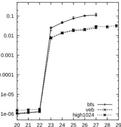
In Figure 8, we look at the performance of the lay-outs as our memory requirement exceeds main memory. As said, for this experiment we booted the machine in such a way that only 32 MB of RAM was available. We compare the van Emde Boas layout, the usual BFS layout, and a 1024-ary version version of it, optimized for the page size of the virtual memory. The keys of a 1024-ary nodes are stored in sorted order, and a node is searched by a fixed, inlined decision tree. We measure the time for random searches on a static tree.
a factor of five outside. The tree optimized for page size is the best outside main memory, but looses by a factor of two inside. Remarkably, the van Emde Boas layout is on par with the best throughout the range.
4.3 Conclusion. From the experiments reported in this paper, it is apparent that the effects of the memory hierarchy in todays computers play a dominant role for the running time of tree search algorithms, already for sizes of trees well within main memory.
It also appears that in the area of search trees, the nice theoretical properties of cache obliviousness seems to carry over into practice: in our experiments, the van Emde Boas layout was competitive with cache aware structures, was better than structures not optimized for
memory access for all but the smallestn, and behaved
robustly over several levels of the memory hierarchy. One further observation is that the effects from the space saving and increase in fanout caused by implicit layouts are notable.
Finally, the method for dynamic cache oblivious search tree suggested in this paper seems practical, not only in terms of implementation effort but also in terms of running time.
References
[1] A. Aggarwal and J. S. Vitter. The input/output com-plexity of sorting and related problems. Communica-tions of the ACM, 31(9):1116–1127, Sept. 1988.
[2] A. Andersson and T. W. Lai. Fast updating of
well-balanced trees. In SWAT 90, 2nd Scandinavian Workshop on Algorithm Theory, volume 447 ofLecture Notes in Computer Science, pages 111–121. Springer, 1990.
[3] L. Arge and J. S. Vitter. Optimal dynamic interval management in external memory. InProc. 37th Ann. Symp. on Foundations of Computer Science, pages 560–569. IEEE Computer Society Press, 1996. [4] R. Bayer and E. McCreight. Organization and
main-tenance of large ordered indexes. Acta Informatica, 1:173–189, 1972.
[5] M. A. Bender, E. Demaine, and M. Farach-Colton. Cache-oblivious B-trees. In Proc. 41st Ann. Symp. on Foundations of Computer Science, pages 399–409. IEEE Computer Society Press, 2000.
[6] M. A. Bender, Z. Duan, J. Iacono, and J. Wu. A locality-preserving cache-oblivious dynamic dictionary. In Proc. 13th Ann. ACM-SIAM Symp. on Discrete Algorithms, 2002.
[7] S. Carlsson, P. V. Poblete, and J. I. Munro. An implicit binomial queue with constant insertion time. In Proc. 1st Scandinavian Workshop on Algorithm Theory, volume 318 of Lecture Notes in Computer Science, pages 1–13. Springer Verlag, Berlin, 1988.
[8] S. Chatterjee, V. V. Jain, A. R. Lebeck, S. Mundhra, and M. Thottethodi. Nonlinear array layouts for hierarchical memory systems. In Proceedings of the 1999 Conference on Supercomputing, ACM SIGARCH, pages 444–453. ACM Press, 1999.
[9] P. F. Dietz and J. Zhang. Lower bounds for monotonic list labeling. In J. R. Gilbert and R. G. Karlsson,
editors, SWAT 90, 2nd Scandinavian Workshop on
Algorithm Theory, volume 447 of Lecture Notes in Computer Science, pages 173–180. Springer, 1990. [10] R. Fagerberg. The complexity of rebalancing a binary
search tree. FSTTCS: Foundations of Software Tech-nology and Theoretical Computer Science, 19, 1999. [11] A. Fiat, J. I. Munro, M. Naor, A. A. Sch¨affer, J. P.
Schmidt, and A. Siegel. An implicit data structure for searching a multikey table in logarithmic time.
Journal of Computer and System Sciences, 43(3):406– 424, 1991.
[12] M. Frigo, C. E. Leiserson, H. Prokop, and S. Ra-machandran. Cache-oblivious algorithms. In40th An-nual Symposium on Foundations of Computer Science, pages 285–297. IEEE Computer Society Press, 1999. [13] J. L. Hennessy and D. A. Patterson. Computer
Archi-tecture: A Quantitative Approach. Morgan Kaufmann, second edition, 1996.
[14] A. Itai, A. G. Konheim, and M. Rodeh. A sparse table implementation of priority queues. InAutomata, Languages and Programming, 8th Colloquium, volume 115 ofLecture Notes in Computer Science, pages 417– 431. Springer-Verlag, 1981.
[15] D. W. Jones. An Empirical Comparison of Priority-Queue and Event-Set Implementations. Communica-tions of the ACM, 29(4):300–311, 1986.
[16] A. LaMarca and R. E. Ladner. The influence of
caches on the performance of heaps. ACM Journal of Experimental Algorithms, 1:4, 1996.
[17] K. Mehlhorn and S. N¨aher. LEDA: A Platform of Combinatorial and Geometric Computing. Cambridge University Press, 1999.
[18] J. I. Munro. An implicit data structure supporting in-sertion, deletion, and search inO(log2n) time. Journal
of Computer and System Sciences, 33(1):66–74, 1986. [19] H. Prokop. Cache-oblivious algorithms. Master’s
thesis, Massachusetts Institute of Technology, June 1999.
[20] N. Rahman, R. Cole, and R. Raman. Optimized pre-decessor data structures for internal memory. InWAE 2001, 5th Int. Workshop on Algorithm Engineering, volume 2141 ofLNCS, pages 67–78. Springer, 2001. [21] P. van Emde Boas. Preserving order in a forest in less
than logarithmic time and linear space. Inf. Process. Lett., 6:80–82, 1977.
[22] P. van Emde Boas, R. Kaas, and E. Zijlstra. Design and implementation of an efficient priority queue.
Mathematical Systems Theory, 10:99–127, 1977. [23] J. W. J. Williams. Algorithm 232: Heapsort.